
Electro-Optical Nose for Indoor Air Quality Monitoring
by
 , , , , and
Víctor González
,
Félix Meléndez
 ,
,
Patricia Arroyo
,
Javier Godoy
,
Fernando Díaz
,
José Ignacio Suárez
and
Jesús Lozano
*
Industrial Engineering School, University of Extremadura, 06006 Badajoz, Spain
*
Author to whom correspondence should be addressed.
Chemosensors 2023, 11(10), 535; https://doi.org/10.3390/chemosensors11100535
Submission received: 24 August 2023
/
Revised: 6 October 2023
/
Accepted: 9 October 2023
/
Published: 11 October 2023
(This article belongs to the Collection Recent Advances in Multifunctional Sensing Technology for Gas Analysis)
Abstract
:Nowadays, indoor air pollution is a major problem that affects human health. For that reason, measuring indoor air quality has an increasing interest. Electronic noses are low-cost instruments (compared with reference methods) capable of measuring air components and pollutants at different concentrations. In this paper, an electro-optical nose (electronic nose that includes optical sensors) with non-dispersive infrared sensors and metal oxide semiconductor sensors is used to measure gases that affect indoor air quality. To validate the developed prototype, different gas mixtures (CH4 and CO2) with variable concentrations and humidity values are generated to confirm the discrimination capabilities of the device. Principal Component Analysis (PCA) was used for dimensionality reduction purposes to show the measurements in a plot. Partial Least Squares Regression (PLS) was also performed to calculate the predictive capabilities of the device. PCA results using all the measurements from all the sensors obtained PC1 = 47% and PC2 = 10%; results are improved using only the relevant information of the sensors obtaining PC1 = 79% and PC2 = 9%. PLS results with CH4 using only MOX sensors received an RMSE = 118.8. When using NDIR and MOX sensors, RMSE is reduced to 19.868; this tendency is also observed in CO2 (RMSE = 116.35 with MOX and RMSE = 20.548 with MOX and NDIR). The results confirm that the designed electro-optical nose can detect different gas concentrations and discriminate between different mixtures of gases; also, a better correlation and dispersion is achieved. The addition of NDIR sensors gives better results in measuring specific gases, discrimination, and concentration prediction capabilities in comparison to electronic noses with metal oxide gas sensors.
Keywords:
electronic nose; electro-optical nose; indoor air quality; metal oxide; non-dispersive infrared detector; PCA; PLS; CO2; CH4; VOCS1. Introduction
In recent years, air pollution has been a major problem that can negatively affect human health. Indoor air pollution affects schools, hospitals, offices, houses, etc. Indoor pollutants include carbon dioxide (CO2) and volatile organic compounds, also known as VOCs (among others), as explained in the work made by Taştan et al. [1]. One of the main CO2 sources is human breath, so the number of occupants and ventilation are important factors in the concentration. The study by Lowther et al. [2] found that although some studies have proved that concentrations less than 5000 ppm have effects on human health and it is associated with reduced cognitive performance and sick-building syndrome, it is not clear if it has a direct impact on health. However, Azuma et al. [3] found that concentrations above 500 ppm are related to physiological changes such as an increase in blood pressure, an increase in heart rate, and an increase in peripherical blood circulation. Concentrations above 1000 ppm are related to problems in cognitive performance and concentrations above 10,000 ppm are related to an increase in respiratory rate and brain blood flow, among others. With that knowledge, different levels of indoor air quality can be used. The Spanish legislation for thermal facilities in buildings [4] shows four different levels of indoor air quality comprising 350 ppm of CO2, meaning an optimum-quality level; 500 ppm, a good-quality level; 800 ppm, a medium-quality level; and 1200 ppm, a poor-quality level, which is not recommended, and should not be applied.
As a volatile organic compound, methane (CH4) is a precursor to tropospheric O3, which is associated with adverse effects on human health, including asthma, reduced lung function, and chronic obstructive pulmonary disease (COPD), as explained by Mar et al. [5]. A study by Dingenen et al. [6] estimated that, relative to 2010 exposure levels, high CH4 emissions would lead to 40,000 to 90,000 deaths related to O3 in 2050. However, mitigation scenarios would decrease mortality from 30,000 to 40,000. Following the current legislation about the exposition of chemical agents, according to the Spanish Ministry of Work’s technical guidelines [7], the secure exposure level of CH4 in a working day of 8 h and 40 h per week is 1000 ppm.
To measure air compounds, electronic noses are designed as instruments capable of recognizing simple and complex odors. An electronic nose is formed using an array of chemical sensors that transform an odor into an electrical signal, an acquisition system to measure all the signals, and finally, a pattern recognition system to classify the samples [8]. The most important types of sensors in electronic noses are optical, surface acoustic wave, electrochemical, catalytic, and semiconductor, as explained by Park et al. [9]. The most used sensors are semiconductor metal oxides (MOX), as they have a rapid response, low consumption, and they are low-cost. MOX sensors are made up of a metal oxide film doped with other compounds such as tungsten trioxide or zinc oxide (n-type) or nickel oxide (p-type). When it contacts the volatiles in the air, a depletion layer is formed, resulting in a change in conductivity. The main drawbacks of these types of sensors are the low selectivity and sensitivity, as they react to different compounds in the environment and their response is affected by humidity changes producing a drift (Arroyo et al. [10] and Meng Yan et al. [11]). According to Dinh et al. [12], non-dispersive infrared (NDIR) sensors are optical sensors and they have high selectivity and sensibility but they are not optimal for miniaturized designs. NDIR sensors target the wavelength absorption in the infrared spectrum to identify a particular gas such as carbon monoxide (CO), carbon dioxide (CO2), methane (CH4), etc.
Various works have been published on NDIR and MOX sensors. They include fire detection [13], gas discrimination [14], food applications [15], and localization of victims in confined spaces [16]. The previously cited works only used CO2 NDIR sensors. However, other works, such as Rutolo et al. [17], used CO2 and CH4 NDIR sensors in addition to electrochemical sensors to detect diseases in potatoes. Also, Wang et al. [18] used an array of five NDIR sensors, with CH4 among them, to monitor the composition of natural gas.
Related to indoor air quality monitoring, Jo et.al [19] developed a device with an NDIR sensor to detect CO2, a semiconductor sensor for CO, a laser dust sensor, a humidity sensor, and a VOC sensor. Air quality data were transferred wirelessly to a server, and an LED strip changed the color if the air quality changed. In another work [1], an IoT device based on an ESP32 module with dust sensors, a CO2 NDIR sensor, a MOX sensor, and a humidity and temperature sensor were developed. They concluded that air quality was related to the number of people in a specific are and that the activities that took place in that area changed the gas concentration. On the other hand, Baldelli [20] used a matrix composed of three MOX sensors, a CO2 NDIR sensor, and an electrochemical sensor. A linear correlation between calculated concentrations and measurements from sensors was found.
The electro-optical nose is a concept introduced by Tibuzzi et al. [21] as an electronic nose sensitive to the light spectrum, made up of a light source and photodiodes coated with different sensitive materials. The sensitive film acts as an optical filter for the emitter light, and the variation in current is due to exposure to VOCs. Other works that used the denomination of electro-optical-nose are [22,23], which are related to this work. They used a combination of specific NDIR and non-specific MOX sensors to obtain an orthogonal array of sensors.
The aim of this work is to detect different concentrations of gases such as CO2 and CH4 that affect indoor air quality using an electro-optical nose with NDIR and MOX sensors. Firstly, preliminary measurements at different concentrations are completed, and values from the legislation presented in [4,7] are used as a reference to validate the system. Secondly, the response of the system to variations in humidity was performed. Finally, the capability of discriminating different gases at different concentrations was measured to test the system in a more complex mixture. The developed electro-optical nose (NEONOSE) from Meléndez et al.’s [23] previous works was used. It has a matrix of five MOX sensors and seven NDIR sensors. The main advantages of this electronic nose are the combination of the non-specific response of MOX sensors, the specific response of the NDIR sensors, and the large number of signals provided by all the sensors.
2. Materials and Methods
2.1. Gas Preparation
Compressed CH4 5000 ppm, synthetic air (N2: 50–80% and O2: 20–50%), and CO2 5000 ppm gas bottles were provided by NIPPON GASES ESPAÑA S.L.U (Madrid, Spain). Gases were mixed by a gas mixing unit to get different concentrations of each gas and mixture. It has four different channels for input gas. The gas mixing unit uses a PLC to control and automatize the process. Each gas flow is controlled by a mass flow controller and gas is mixed with a manifold. It allows humidity control with a humidity generator, with an operating range of 5 to 80%.
2.2. Sensory System
Electro-optical nose (NEONOSE), developed by the perception and intelligent systems research group from Universidad de Extremadura (PSI-UNEX), was used. The printed circuit boards of the electronic nose are presented in Figure 1. NEONOSE is formed using two boards that contain NDIR and MOX sensors. These boards are communicated to each other via SPI.
Figure 2 shows a block diagram of the electronic nose. The main board is formed with five MOX sensors and one NDIR type, which are communicated with the microcontroller (PIC32MM0256GPM048 Microchip) via I2C. Moreover, it sends the data received by all the sensors via Bluetooth to a smartphone.
The secondary board is formed completely using NDIR sensors. Some sensors have an analog response, so the signal is processed via operational amplifiers and converted to digital signals via A/D converters. Others send data digitally to the microcontroller via UART. All the data are sent from the secondary board to the main board via SPI.
2.3. Electronic Nose Setup
The electronic nose was controlled with an Android app and data were sent via Bluetooth to a smart phone. Parameters such as absorption and desorption time can be configured (this feature is not used in this work), as well as the sampling time of the sensors and an alarm sound to inform the change between the sample and air.
As the main interests of this work are the detection and discrimination of different gases with different concentrations, a gas mixing unit is used. The gas mixing unit is controlled with a LabView application running on Windows. Communication between the computer and gas mixing unit is performed using a multimeter Keithley 2700.
The application allows to change the gas concentration (ppm) and the relative humidity; moreover, step time and concentration of different steps can be configured. Connection to gas channels was performed as follows: Channel 1 (CO2) and Channel 3 (CH4) were connected to bottle samples, while Channel 2 and Channel 4 were connected to dry and wet air, respectively.
The gas mixing unit takes dry air, and mixes both dry air and sample, finally the mix flows through a humidity generator. Output gas is the addition of the percentage of wet gas, the ratio between the step concentration of the gas and the concentration of the bottle, and finally, the rest is dry air. Output gas is carried from the gas mixing unit to a polypropylene gas cell in the electronic nose, and a flow meter is always used to check the constant airflow to the system. Furthermore, it should also be noted that the design of the cell makes the two boards face each other.
A data acquisition card, (DAQ) NATIONAL INSTRUMENTS USB-6009, is connected to synchronize the electronic nose and the LabView program. When the countdown in each concentration step is zero, the program sends a 5-volt signal through the DAQ. This signal is conditioned with a voltage divider to 3.3 volts, and the microcontroller reads this signal to change between the sample and air readings. The electronic nose sends the sample/air data measured from the sensors to the Android app. Figure 3 shows a detailed view of the measurement block diagram.
2.4. Preliminary Measurements
A total of 14 CO2 and CH4 steps were completed in a range from 3000 ppm to 100 ppm (3000 ppm, 2500 ppm, 2000 ppm, 1500 ppm, 1000 ppm, 900 ppm, 800 ppm, 700 ppm, 600 ppm, 500 ppm, 400 ppm, 300 ppm, 200 ppm, 100 ppm) to get the best range of the sensors’ response; also the values of the legislation mentioned in Section 1 in [4,7] are included in this range. Measurements were completed with an absorption time (sample) of 4 min and 12 min of desorption time (air) to reach a good stationary response of all sensors. A sample time of 2000 ms was configured and a 40% relative humidity was selected.
2.5. Mixture of CO2 and CH4 Measurements
Once preliminary measurements are performed and an appropriate measurement range is met, a mixture of CO2 and CH4, as shown in Table 3, is made to test the discrimination capabilities of the electronic nose. Experimental conditions were similar to preliminary measurements. Ten repetitions per step were performed so that the repeatability of the measurements could be analyzed.
2.6. Humidity Measurements
Different humidity measurements is performed to see if the response of the whole system is altered with variations of relative humidity. Experimental conditions are the same as described above. However, the concentration of gases is fixed, and different steps of humidity are programmed, experiments are performed with target gases because NDIR sensors respond specifically to them, and only dry/wet air will not have a response. The values are chosen according to the relative humidity range described in [4], and are the following: 40%, 50%, and 60%. In addition, a step of 70% relative humidity is included, although this step is out of range. It is used to test non-optimal conditions.
2.7. Data Analysis
A total of 37 variables from all the sensors are measured, and all the signals and their kind are illustrated in Table 1 and Table 2. The total of samples measured in both absorption and desorption time ascends to 5179 samples in each concentration step repetition.
A characteristic value of the response of each sensor is needed for each performed repetition; to extract the characteristics of the measurements, the algorithm from Equation (1) is used in pretreatment.
where MAX is the maximum value reached in the repetition and MIN is the minimum. Processed data are stored in a matrix of characteristic values where the number of rows is the number of measurements and the columns are the number of sensors; dimensions of the matrix are 70 × 37, considering that 7 different concentration steps are applied, and each step has 10 repetitions.
Due to the number of data collected in the characteristic matrix, mathematical algorithms are required to process all the information. Dimensionality reduction is carried out using Principal Component Analysis (PCA) to classify the samples. This technique describes a dataset in terms of new non-correlated variables (components). Components are sorted by the amount of variance they represent. Therefore, this technique is useful for reducing the dimensionality and the redundancy of the collected data [24].
To generate prediction models, Partial Least Square (PLS) is used [25]. In PLS, a linear regression is made with the measured parameters and predicted parameters to see the correlation between them. The leave-one-out cross-validation method was used. This validation method takes one of the repetitions as the validation data and the rest as training.
PCA and PLS analyses are performed in MATLAB R2022b with an application developed by the research group.
3. Results
3.1. Preliminary CO2 Measurements Results
Temporary results of some sensors are analyzed. Firstly, the IAQ (indoor air quality) response of ZMOD4410 is illustrated in Figure 4. The ranges of quality are given by the manufacturer in Table 4, and these values are measured based on TVOCs. Knowing these values, when reference air is introduced in the electro-optical nose (when there are no steps), the IAQ value corresponds to very good air quality (Level 1). However, when a 3000 ppm step concentration is introduced, air quality moves to a good-quality level (Level 2), and this rate is maintained until the 1500 ppm step; concentrations below these values correspond to a very good quality level.
On the other hand, CCS811 responses to CO2 and ZMOD4410 are analyzed in Figure 5, and these values are measured based on TVOCs. As it is shown in Figure 5a, the ZMOD4410 tendency is consistent with Figure 4. The higher concentration of CO2 (3000, 2500, 2000, 1500 ppm) corresponds to higher CO2 measurements, and it is equivalent to the IAQ ratings. In addition, values of response are close to 400 ppm when reference air is introduced because of a baseline calibration made by the sensor around that value.
In Figure 5b, responses of CCS811 are shown. It can be seen that the sensor responds to the entire concentration range, and the minimum value changes to approximately 400 ppm (values reached when reference air) because the sensor performs a baseline calibration around this value, similarly to the ZMOD4410 response.
Concerning the NDIR sensors, CO2 concentrations must be higher if a response is desired from all those implemented in the electronic nose, as their lower detection limit is even higher. However, the SCD40 sensor has the best performance of all CO2 sensors, managing to react to all the steps, as shown in Figure 6a. As it was explained in MOX sensors, values of measurements start with a calibrated value (around 500 ppm in this case). These results are consistent with the measurement range provided by the manufacturer (0–40,000 ppm). If the response of the CH4 NDIR sensor SJH5 is plotted, as can be seen in Figure 6b, it does not have a clear response because it does not respond to CO2.
3.2. Preliminary CH4 Measurements Results
As shown in Figure 7, ZMOD4410 and CCS811 respond in the entire concentration range of CH4, as it is a volatile organic compound. The maximum value of TVOC detected with CCS811 is 1187 ppb, according to the manufacturer, and 10,000 ppb with the ZMOD4410. Both responses meet the ranges.
The SJH5 NDIR sensor is the only one of its kind that responds to CH4, and the response is shown in Figure 8a. The only step that does not have any response corresponds to 100 ppm. According to the manufacturer, it responds from 0 to 50,000 ppm, so its limit detection is 100 ppm. Also, like the other sensors, SJH5 has a calibration set point for measurements. In Figure 8b, the response of SCD40 can also be seen, and it does not have a clear response; its value is close to the calibration reference value due to the target gas of this sensor being CO2, and it will not respond to other gases.
3.3. Humidity Measurements
In this case, different steps of humidity are introduced in the electro-optical nose at constant concentrations (1500 ppm of CO2 and 1500 ppm of CH4). In Figure 9, the response of the NDIR SCD40 sensor and the MOX sensor BME680 to CO2 is shown. As can be seen, the response of the MOX sensor is highly influenced by humidity (Figure 9a). The response decreases as humidity increases. Also, drift is appreciated. However, the NDIR sensor response is more stable (Figure 9b). In Figure 10, the response to CH4 is shown, and the response is similar to Figure 9 because the MOX sensor remains with a huge drift, and the response of NDIR remains almost constant.
3.4. Mixture of CO2 and CH4 Measurements
3.4.1. PCA Results
To understand all the measured data, a PCA was performed. Figure 11 shows a PCA with all the sensor signals, showing an explained variance of 47% for PC1 and 10% for PC2. There is a good separation between clusters and correlation between the concentration of the mixture and the PC1 can also be observed; higher CO2 concentration samples are located in the right side on the PC1, and higher CH4 concentration samples are located on the left side of PC1. Although groups are dispersed, when the concentration in CH4 reaches 2000 ppm, overlapping can be seen. Such problems could be related to NDIR sensors, as the only ones that provide reliable information are the SCD40 and SJH5. If a 3D plot of the PCA is represented, as shown in Figure 12, it can be seen that the overlapping occurs due to the missing information from the third component.
Figure 13 shows the load plot of all the sensors. The load plot shows how important the contribution of a variable is in a PCA. The most important variables in PC2 are S24 (corresponding to IRC_A1), S26, S27, S28 (corresponding to IRC_AT), S29, S30 (corresponding to IRM_AT), and S36 (corresponding to IRNET); therefore, they have a negative effect in relation to the total response and cause a bigger dispersion. If the information of these signals is deleted from the analysis, this will eliminate the masking produced by them, and the correlation will improve. Further analysis in this section will aim to improve the PCA with reliable information from MOX sensors and NDIR sensors.
If only the response from MOX sensors is used (S4, S5, S6, S7, S8, S9, S10, S11, S12, S13, S14, S15, S16, S17), the PCA (Figure 14) shows better discrimination of the groups, with a 78% explained variance for PC1; furthermore, the dispersion in clusters is reduced as variables from the NDIR sensors that are not responding to these concentrations are removed. Also, variables from temperature and relative humidity are not used because they do not add useful information about the mixture.
By adding the variables from the NDIR sensors (SCD40 and SJH5) that have a response (S20, S32, and S33), as shown in Figure 15, it can be seen that the dispersion in clusters is reduced, and the correlation between PC1 and the concentration is clearer than in the analysis made with all the sensor’s responses, as there are not overlapped groups. While the higher CO2 concentrations are located on the left side of PC1, the higher CH4 concentrations are located on the right side of PC1. It can also be seen that the mixture with equal concentrations of CO2 and CH4 is almost centered in the PCA.
3.4.2. PLS Results
PLS analysis was performed on the ten repetitions using the leave-one-out cross-validation method. A PLS was performed using CO2 and CH4 results with MOX sensors’ variables used in a PCA. As is shown in Figure 16, there is a good correlation between the predicted and measured variables in CH4 and CO2. However, the dispersion is significant, as explained by the root mean square error (RMS). This value can be reduced with the addition of NDIR sensors’ variables used at the end of the PCA, as can be seen in Figure 17. Moreover, the addition of specific sensors also improves the correlation, giving slightly improved predictions.
4. Discussion
In this study, an electro-optical nose that combines different technologies of commercial sensors (MOX and NDIR) is used. Moreover, the design of the electro-optical nose allows different sensors to be configured and changed depending on the required application.
The device can detect concentrations presented in the legislation related to indoor air quality [4,7]. IAQ parameters measured among other parameters from MOX sensors show that the level of air quality improves as the concentration of CO2 decreases. It is important to note that the air quality classification may differ from the one presented in [4] because it is based on air quality ranges outlined in [26]. However, there are some limitations in the electro-optical nose related to the non-specific response of MOX sensors.
MOX sensors exhibited responses to CO2 and CH4, although they typically do not measure CO2 directly. Instead, they utilize algorithms to estimate CO2 from the TVOCs that are detected. Detecting CO2 using MOX sensors can be challenging because CO2 is a stable gas, as described by Staerz et al. [27]. Their response is caused by the complex interactions between the gases present and the sensor’s surface morphology, as explained by Moumen et al. [28].
As Arroyo et al. [10] found, when MOX sensors are exposed to different humidity conditions their response can experience drift because they can adsorb water vapor, as explained in [11]. Future studies should make multivariable analyses to account for the influence of humidity on these sensors and explore different ways to mitigate drift in their responses.
The addition of more sensors and other technologies improves the reliability of the system. NDIR sensors reduce the limitations imposed by MOX sensors, since they show a specific response to the target gases they are designed for (CH4 and CO2 (in this work)), as explained by Dinh et al. [12]. Moreover, the problems associated with the humidity drift are negligible, as minor variations of NDIR measurements, when measuring humidity, could be related to the heating of the sensors.
When the PCA analysis is performed with a mixture of CO2 and CH4, good discrimination using MOX sensors is achieved despite their non-specific response; all the signals provided by them compensate for these effects, this providing a good discrimination. In addition, PLS shows a good correlation using MOX sensors too.
An improvement in the PCA score is reached when NDIR sensors are added, resulting in a better correlation between PC1 and the concentration. Also, the PLS results showed lower dispersion, as their specific response adds information that MOX sensors cannot provide. However, it is important to note that some NDIR sensors do not respond to the studied measurement range, and require higher concentrations. These non-responsive sensors did not significantly contribute to the PCA analysis and were ultimately excluded from the analysis. Nevertheless, they are retained in the electronic nose for future measurements in leakage applications.
5. Conclusions
In this work, an electro-optical nose with NDIR and MOX sensors to measure indoor air quality is developed. Different gases, concentrations, and mixtures are used to validate the electronic nose in lab conditions as a first approach.
Preliminary measurements on individual gases show a good response of both NDIR and MOX sensors. MOX sensors respond to both CH4 and CO2. NDIR sensors give a specific response to CH4 and CO2, improving the response of the whole system and accuracy. The measurements of concentrations meet the values from the legislation mentioned in Section 1; therefore, the device can be used to measure indoor air quality.
Humidity measurements show that MOX sensors vary their response to humidity changes at constant concentrations. However, the addition of NDIR sensors could improve the reliability of the system because their response is more stable.
The PCA analysis of mixtures shows that MOX sensors can discriminate different gases at different concentrations. However, the discrimination capabilities of the electronic nose can be improved with the addition of NDIR sensors because of their specific response to gases.
Finally, PLS results give a good prediction using MOX sensors; correlation and dispersion could be improved by adding NDIR sensors, which is consistent with the results provided with the PCA analysis.
Author Contributions
V.G.: methodology, investigation, and writing; F.M.: software, investigation, and data curation; P.A.: writing—review and editing, visualization, and supervision; J.G., F.D. and J.I.S.: investigation and writing—review and editing; J.L.: investigation, supervision, and funding acquisition. All authors have read and agreed to the published version of the manuscript.
Funding
This research was funded by the Spanish Ministry of Science and Innovation, grant number PID2019-107697RB-C44.
Data Availability Statement
Data of the sensors will be available upon request.
Conflicts of Interest
The authors declare no conflict of interest.
References
- Taştan, M.; Gökozan, H. Real-Time Monitoring of Indoor Air Quality with Internet of Things-Based e-Nose. Appl. Sci. 2019, 9, 3435. [Google Scholar] [CrossRef]
- Lowther, S.D.; Dimitroulopoulou, S.; Foxall, K.; Shrubsole, C.; Cheek, E.; Gadeberg, B.; Sepai, O. Low Level Carbon Dioxide Indoors—A Pollution Indicator or a Pollutant? A Health-Based Perspective. Environments 2021, 8, 125. [Google Scholar] [CrossRef]
- Azuma, K.; Kagi, N.; Yanagi, U.; Osawa, H. Effects of Low-Level Inhalation Exposure to Carbon Dioxide in Indoor Environments: A Short Review on Human Health and Psychomotor Performance. Environ. Int. 2018, 121, 51–56. [Google Scholar] [CrossRef] [PubMed]
- Real Decreto 1027/2007, de 20 de Julio, Por El Que Se Aprueba El Reglamento de Instalaciones Térmicas en Los Edificios. 2007. Available online: https://www.boe.es/eli/es/rd/2007/07/20/1027 (accessed on 23 August 2023).
- Mar, K.A.; Unger, C.; Walderdorff, L.; Butler, T. Beyond CO2 Equivalence: The Impacts of Methane on Climate, Ecosystems, and Health. Environ. Sci. Policy 2022, 134, 127–136. [Google Scholar] [CrossRef]
- Dingenen, V.; Crippa, R. Global Trends of Methane Emissions and Their Impacts on Ozone Concentrations. 2017. Available online: https://op.europa.eu/en/publication-detail/-/publication/c40e6fc4-dbf9-11e8-afb3-01aa75ed71a1/language-en (accessed on 23 August 2023).
- Límites de Exposición Profesional Para Agentes Químicos. 2023. Available online: https://www.Insst.Es/El-Instituto-al-Dia/Limites-de-Exposicion-Profesional-Para-Agentes-Quimicos-2023 (accessed on 23 August 2023).
- Lozano, J.; Santos, J.P.; Horrillo, M.C. Wine Applications with Electronic Noses. In Electronic Noses and Tongues in Food Science; Elsevier Inc.: Amsterdam, The Netherlands, 2016; pp. 137–148. ISBN 9780128004029. [Google Scholar]
- Park, S.Y.; Kim, Y.; Kim, T.; Eom, T.H.; Kim, S.Y.; Jang, H.W. Chemoresistive Materials for Electronic Nose: Progress, Perspectives, and Challenges. InfoMat 2019, 1, 289–316. [Google Scholar] [CrossRef]
- Arroyo, P.; Meléndez, F.; Suárez, J.I.; Herrero, J.L.; Rodríguez, S.; Lozano, J. Electronic Nose with Digital Gas Sensors Connected via Bluetooth to a Smartphone for Air Quality Measurements. Sensors 2020, 20, 786. [Google Scholar] [CrossRef] [PubMed]
- Yan, M.; Wu, Y.; Hua, Z.; Lu, N.; Sun, W.; Zhang, J.; Fan, S. Humidity Compensation Based on Power-Law Response for MOS Sensors to VOCs. Sens. Actuators B Chem. 2021, 334, 129601. [Google Scholar] [CrossRef]
- Dinh, T.V.; Choi, I.Y.; Son, Y.S.; Kim, J.C. A Review on Non-Dispersive Infrared Gas Sensors: Improvement of Sensor Detection Limit and Interference Correction. Sens. Actuators B Chem. 2016, 231, 529–538. [Google Scholar] [CrossRef]
- Solórzano, A.; Fonollosa, J.; Fernández, L.; Eichmann, J.; Marco, S. Fire Detection Using A Gas Sensor Array with Sensor Fusion Algorithms. In Proceedings of the 2017 ISOCS/IEEE International Symposium on Olfaction and Electronic Nose (ISOEN), Montreal, QC, Canada, 28–31 May 2017. [Google Scholar] [CrossRef]
- Xing, Y.; Vincent, T.A.; Cole, M.; Gardner, J.W.; Fan, H.; Bennetts, V.H.; Schaffernicht, E.; Lilienthal, A.J. Mobile Robot Multi-Sensor Unit for Unsupervised Gas Discrimination in Uncontrolled Environments. In Proceedings of the 2017 IEEE SENSORS, Glasgow, UK, 29 October–1 November 2017. [Google Scholar]
- Dang, C.T.; Seiderer, A.; André, E. Theodor: A Step Towards Smart Home Applications with Electronic Noses. In Proceedings of the 5th International Workshop on Sensor-based Activity Recognition and Interaction, Berlin, Germany, 20–21 September 2018. [Google Scholar] [CrossRef]
- Anyfantis, A.; Blionas, S. Design and Development of a Mobile e-Nose Platform for Real Time Victim Localization in Confined Spaces During USaR Operations. In Proceedings of the 2020 IEEE International Instrumentation and Measurement Technology Conference (I2MTC), Dubrovnik, Croatia, 25–28 May 2020. [Google Scholar]
- Rutolo, M.F.; Clarkson, J.P.; Covington, J.A. The Use of an Electronic Nose to Detect Early Signs of Soft-Rot Infection in Potatoes. Biosyst. Eng. 2018, 167, 137–143. [Google Scholar] [CrossRef]
- Wang, J.; Lei, B.; Yang, Z.; Lei, S. Self-Repairing Infrared Electronic Nose Based on Ensemble Learning and PCA Fault Diagnosis. Infrared Phys. Technol. 2022, 127, 104465. [Google Scholar] [CrossRef]
- Jo, J.; Jo, B.; Kim, J.; Kim, S.; Han, W. Development of an IoT-Based Indoor Air Quality Monitoring Platform. J. Sens. 2020, 2020, 8749764. [Google Scholar] [CrossRef]
- Baldelli, A. Evaluation of a Low-Cost Multi-Channel Monitor for Indoor Air Quality through a Novel, Low-Cost, and Reproducible Platform. Meas. Sens. 2021, 17, 59. [Google Scholar] [CrossRef]
- Tibuzzi, A.; Soncini, G.; D’Amico, A.; Di Natale, C.; Paolesse, R.; Macagnano, A.; Zen, A. An Integrated Electro-Optical Nose. In Proceedings of the Sensors and Microsystems, Trento, Italy, 12–14 February 2003; DiNatale, C., DAmico, A., Soncini, G., Ferrario, L., Zen, M., Eds.; World Scientific Publishing Co., Pte. Ltd.: Singapore, 2004; pp. 300–305. [Google Scholar]
- Meléndez, F.; Arroyo, P.; Gómez-Suárez, J.; Santos, J.P.; Lozano, J. Resistive Metal Oxide Combined with Optical Gas Sensor in an Electro-Optical Nose for Odour Monitoring. Chem. Eng. Trans. 2022, 95, 205–210. [Google Scholar] [CrossRef]
- Meléndez, F.; Arroyo, P.; Suárez, J.I.; Carmona, P.; Fernández, J.Á.; Herrero, J.L.; Gómez-Suárez, J.; Carmona, D.; Lozano, J. NanoElectroOptical Nose (NEONOSE) for the Detection of Climate Change Gases. In Proceedings of the 2022 IEEE International Symposium on Olfaction and Electronic Nose (ISOEN), Aveiro, Portugal, 29 May–1 June 2022. [Google Scholar] [CrossRef]
- Esbensen, K.H.; Geladi, P. Principal Component Analysis: Concept, Geometrical Interpretation, Mathematical Background, Algorithms, History, Practice. In Comprehensive Chemometrics: Chemical and Biochemical Data Analysis, VOLS 1-4; Elsevier: Oxford, UK, 2009; pp. A211–A226. ISBN 978-0444-52702-8. [Google Scholar]
- Bayne, C.K. Multivariate Analysis of Quality: An Introduction. Technometrics 2002, 44, 186–187. [Google Scholar] [CrossRef]
- Umweltbundesamt. Beurteilung von Innenraumluftkontaminationen Mittels Referenz-und Richtwerten: Handreichung der Ad-Hoc-Arbeitsgruppe der Innenraumlufthygiene-Kommission des Umweltbundesamtes und der Obersten Landesgesundheitsbehörden. Bundesgesundheitsblatt Gesundheitsforschung Gesundheitsschutz 2007, 50, 990–1005. [Google Scholar] [CrossRef] [PubMed]
- Staerz, A.; Weimar, U.; Barsan, N. Current State of Knowledge on the Metal Oxide Based Gas Sensing Mechanism. Sens. Actuators B Chem. 2022, 358, 131531. [Google Scholar] [CrossRef]
- Moumen, A.; Kumarage, G.C.W.; Comini, E. P-Type Metal Oxide Semiconductor Thin Films: Synthesis and Chemical Sensor Applications. Sensors 2022, 22, 1359. [Google Scholar] [CrossRef] [PubMed]
Figure 1.
NEONOSE-printed circuit boards with electronic components. Left, main board with MOX sensors, microcontroller, and Bluetooth communications. Right, secondary board with optical sensors.
Figure 1.
NEONOSE-printed circuit boards with electronic components. Left, main board with MOX sensors, microcontroller, and Bluetooth communications. Right, secondary board with optical sensors.

Figure 2.
NEONOSE block diagram with the main parts of the electronic PCBs.

Figure 3.
Measurement system block diagram with the main parts of the electronic and pneumatic circuits.
Figure 3.
Measurement system block diagram with the main parts of the electronic and pneumatic circuits.
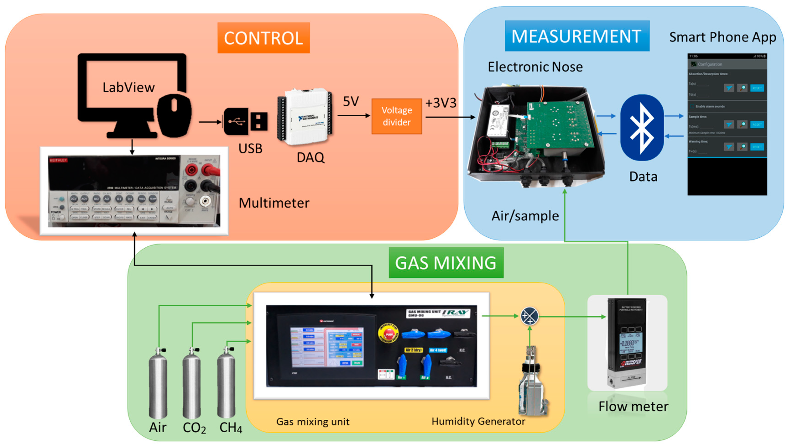
Figure 4.
ZMOD4410 IAQ values vs. different CO2 concentrations.
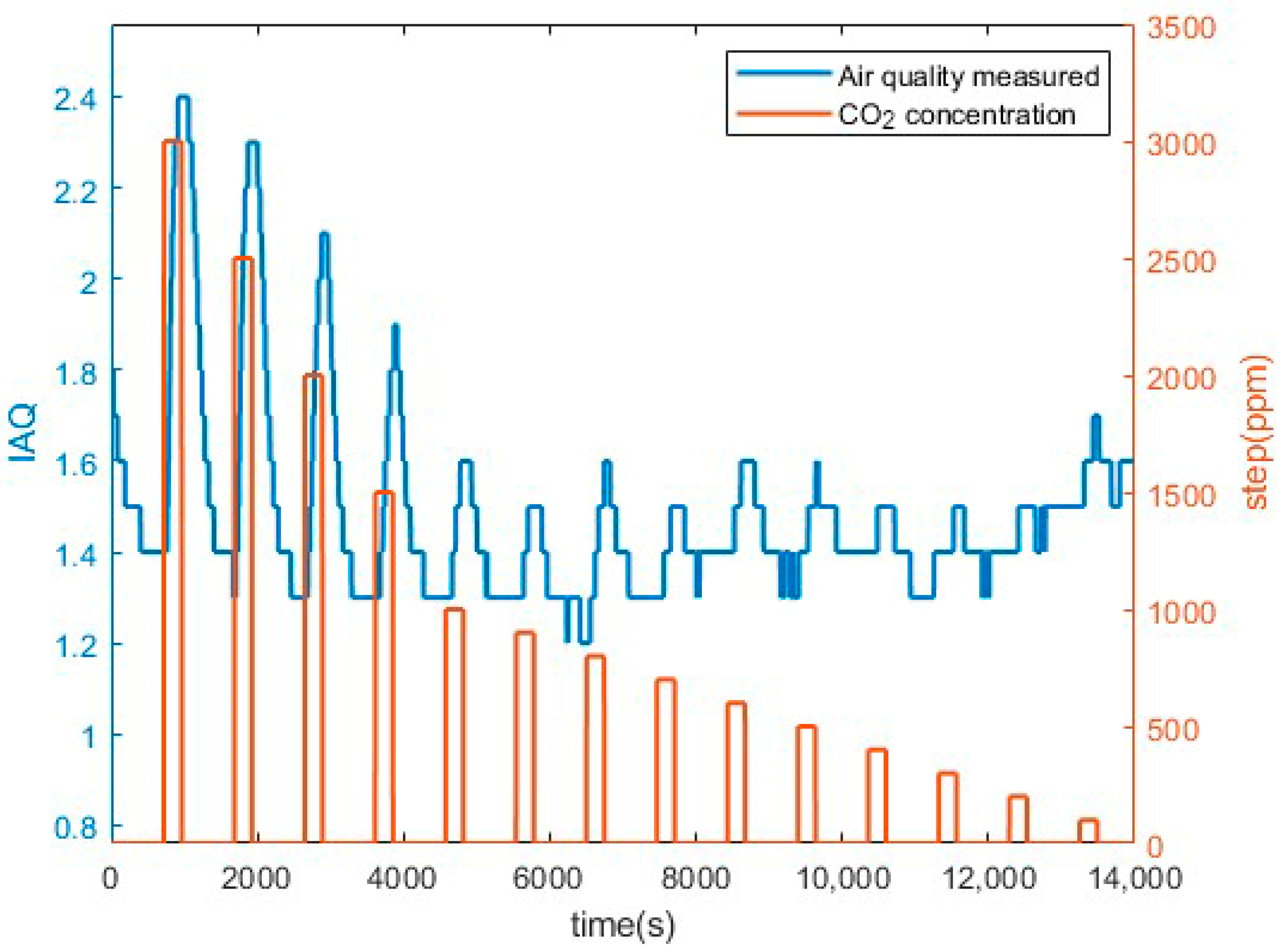
Figure 5.
MOX sensors response to CO2. (a) ZMOD4410 CO2 response; (b) CCS811 CO2 response.
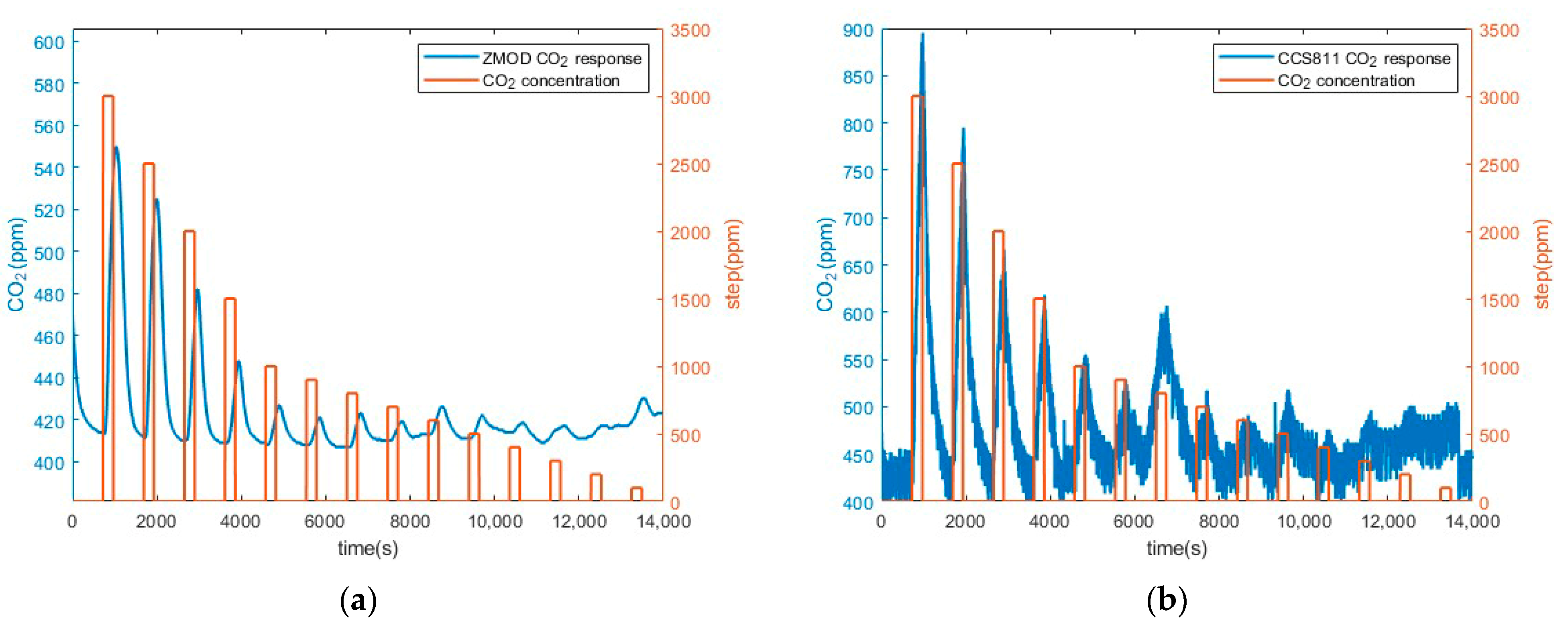
Figure 6.
NDIR sensors response to CO2. (a) SCD40 response. (b) SJH5 response.
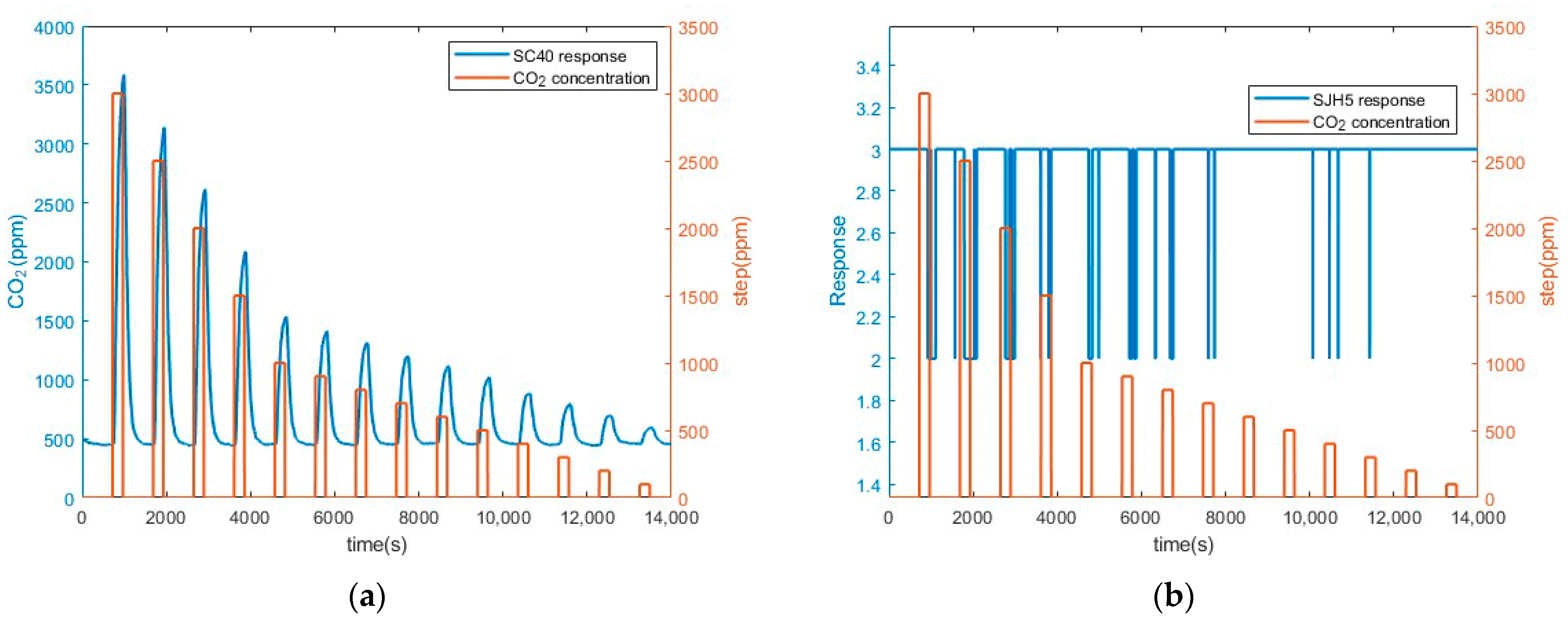
Figure 7.
MOX sensor response to CH4. (a) CCS811 TVOC response; (b) ZMOD TVOC response.
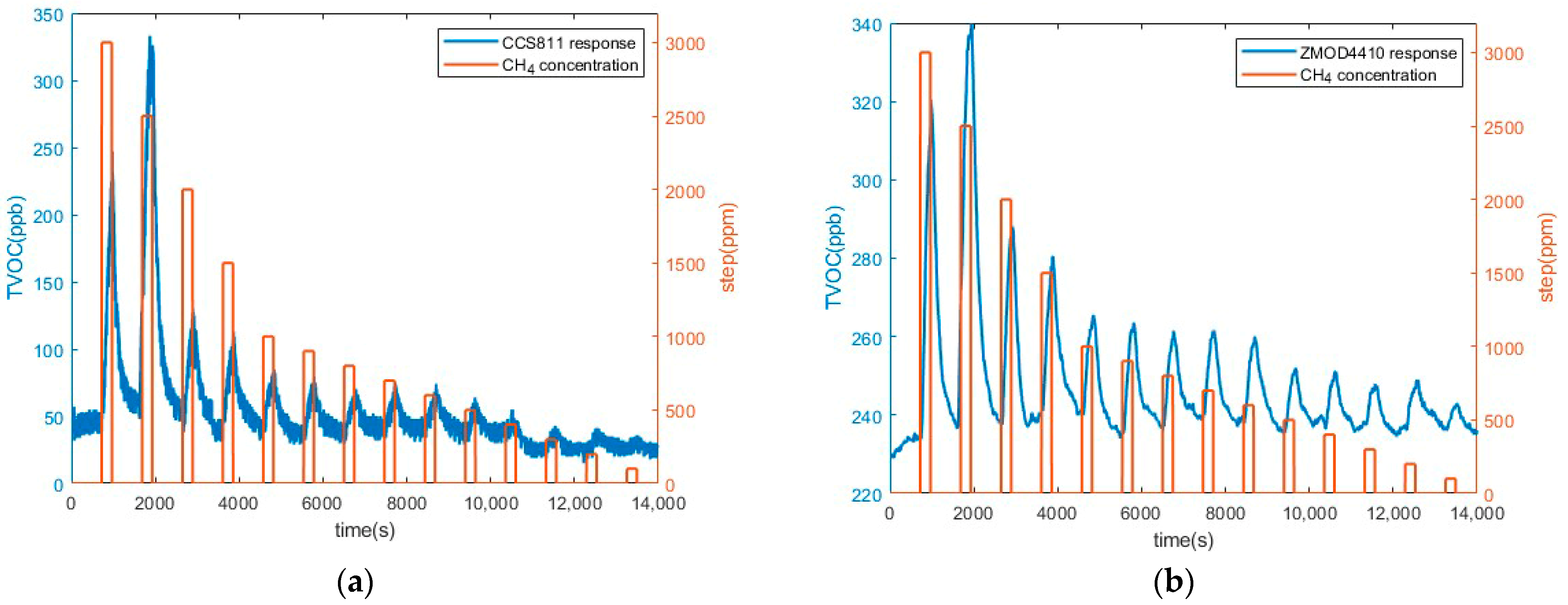
Figure 8.
NDIR sensors response to CH4. (a) SJH5 CH4 response. (b) SCD40 CH4 response.
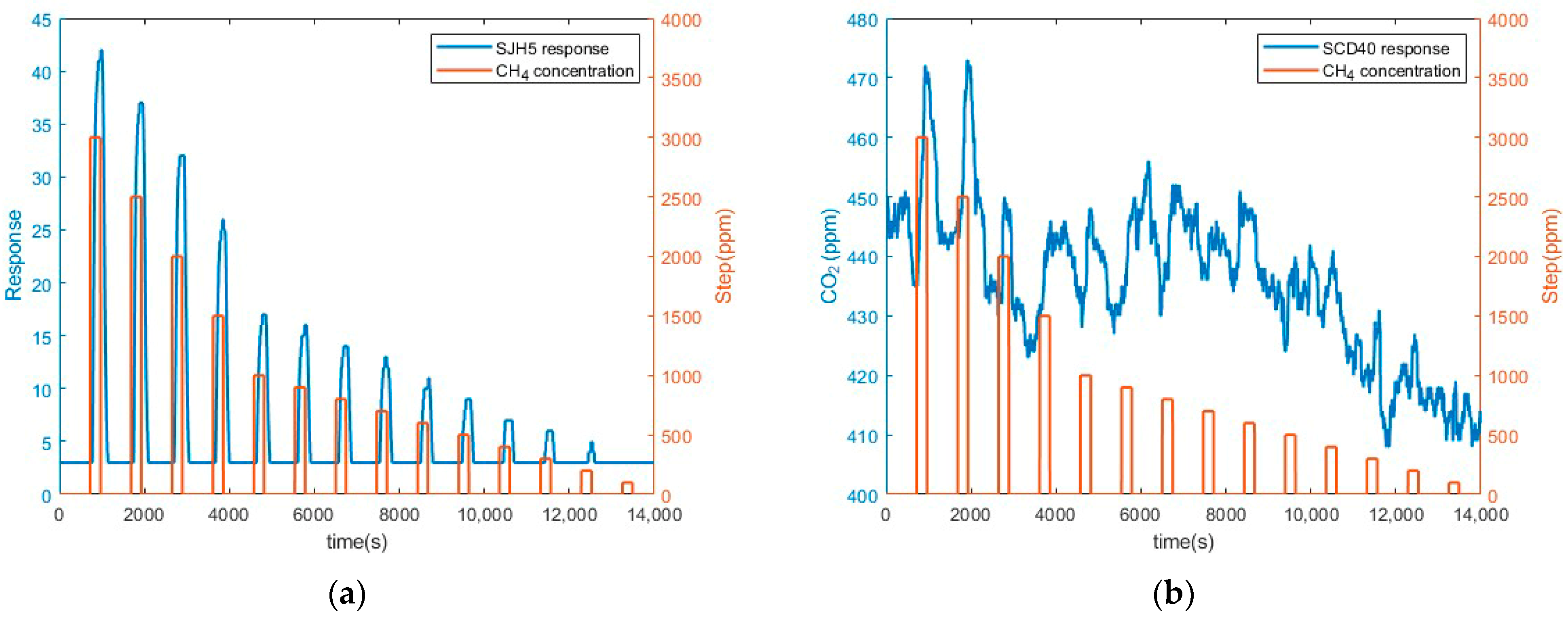
Figure 9.
MOX and NDIR sensors response to humidity changes with CO2. (a) Resistance of BME680; (b) measured CO2 of SCD40.
Figure 9.
MOX and NDIR sensors response to humidity changes with CO2. (a) Resistance of BME680; (b) measured CO2 of SCD40.
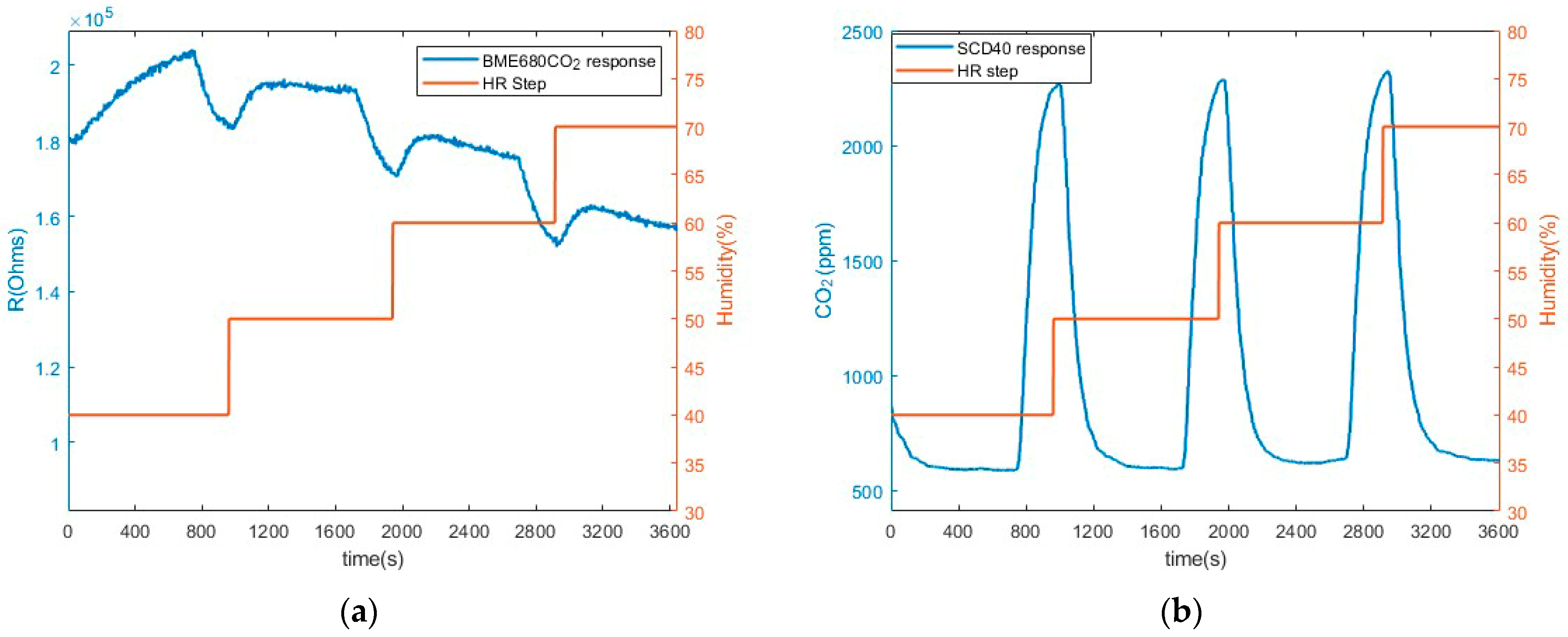
Figure 10.
MOX and NDIR response to humidity changes with CH4. (a) Resistance of BME680; (b) SJH5 response.
Figure 10.
MOX and NDIR response to humidity changes with CH4. (a) Resistance of BME680; (b) SJH5 response.
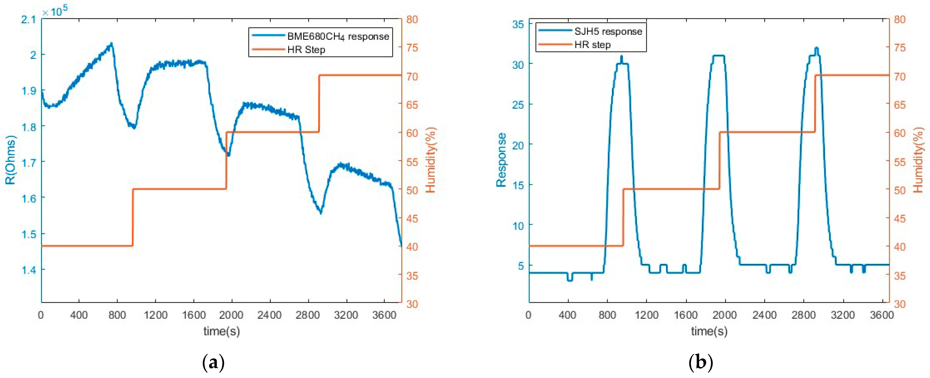
Figure 11.
PCA variable plot with all sensors. A: CO2 = 3000 ppm; B: CH4 = 1000 ppm, CO2 = 2000 ppm; C: CH4 = 1500 ppm, CO2 = 1500 ppm; D: CH4 = 2000 ppm, CO2 = 1000 ppm; E: CH4 = 2500 ppm, CO2 = 500 ppm; F: CH4 = 3000 ppm; G: CH4 = 500 ppm, CO2 = 2500 ppm.
Figure 11.
PCA variable plot with all sensors. A: CO2 = 3000 ppm; B: CH4 = 1000 ppm, CO2 = 2000 ppm; C: CH4 = 1500 ppm, CO2 = 1500 ppm; D: CH4 = 2000 ppm, CO2 = 1000 ppm; E: CH4 = 2500 ppm, CO2 = 500 ppm; F: CH4 = 3000 ppm; G: CH4 = 500 ppm, CO2 = 2500 ppm.
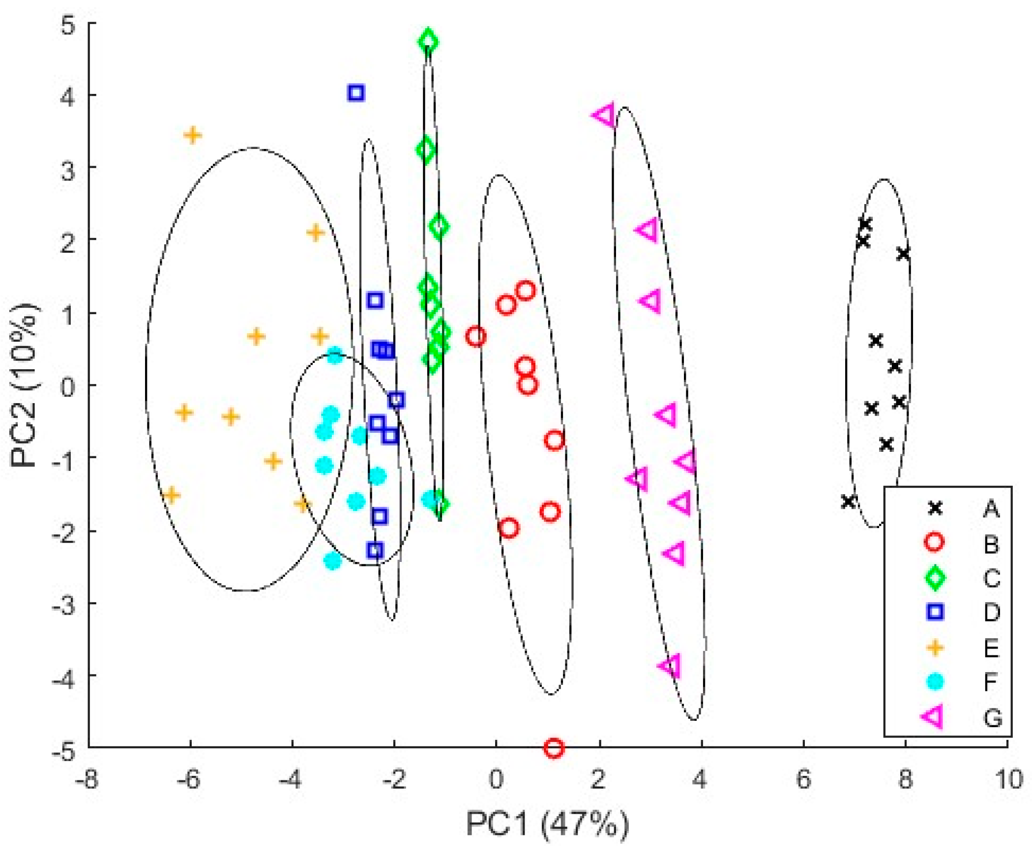
Figure 12.
Three-dimensional plot of the PCA with all variable sensors.

Figure 13.
Loading plot showing sensors contribution from PCA.
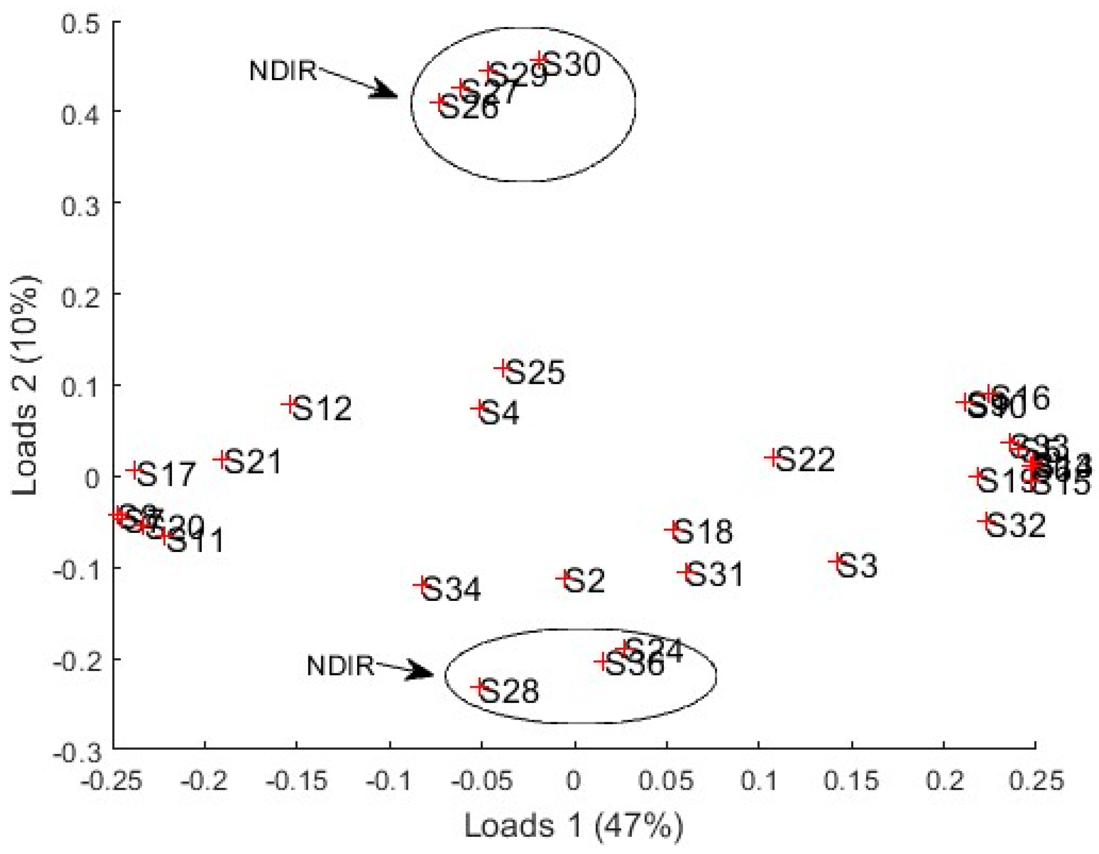
Figure 14.
PCA score plot with MOX sensors. A: CO2 = 3000 ppm; B: CH4 = 1000 ppm, CO2 = 2000 ppm; C: CH4 = 1500 ppm, CO2 = 1500 ppm; D: CH4 = 2000 ppm, CO2 = 1000 ppm; E: CH4 = 2500 ppm, CO2 = 500 ppm; F: CH4 = 3000 ppm; G: CH4 = 500 ppm, CO2 = 2500 ppm.
Figure 14.
PCA score plot with MOX sensors. A: CO2 = 3000 ppm; B: CH4 = 1000 ppm, CO2 = 2000 ppm; C: CH4 = 1500 ppm, CO2 = 1500 ppm; D: CH4 = 2000 ppm, CO2 = 1000 ppm; E: CH4 = 2500 ppm, CO2 = 500 ppm; F: CH4 = 3000 ppm; G: CH4 = 500 ppm, CO2 = 2500 ppm.
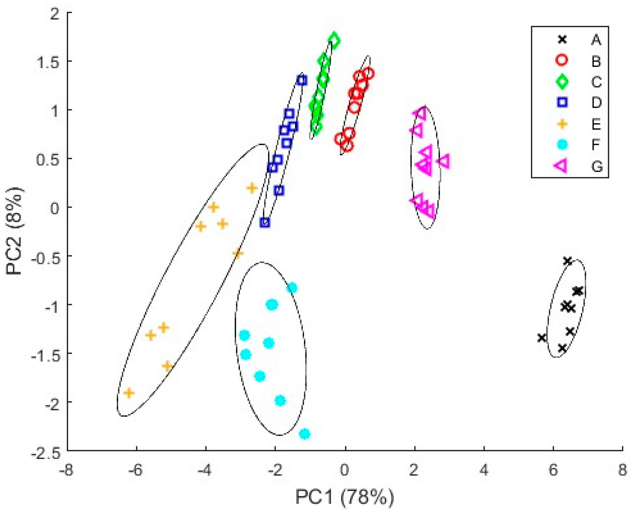
Figure 15.
PCA score plot after adding NDIR (SJH5, SCD40) and MOX sensors. A: CO2 = 3000 ppm; B: CH4 = 1000 ppm, CO2 = 2000 ppm; C: CH4 = 1500 ppm, CO2 = 1500 ppm; D: CH4 = 2000 ppm, CO2 = 1000 ppm; E: CH4 = 2500 ppm, CO2 = 500 ppm; F: CH4 = 3000 ppm; G: CH4 = 500 ppm, CO2 = 2500 ppm.
Figure 15.
PCA score plot after adding NDIR (SJH5, SCD40) and MOX sensors. A: CO2 = 3000 ppm; B: CH4 = 1000 ppm, CO2 = 2000 ppm; C: CH4 = 1500 ppm, CO2 = 1500 ppm; D: CH4 = 2000 ppm, CO2 = 1000 ppm; E: CH4 = 2500 ppm, CO2 = 500 ppm; F: CH4 = 3000 ppm; G: CH4 = 500 ppm, CO2 = 2500 ppm.
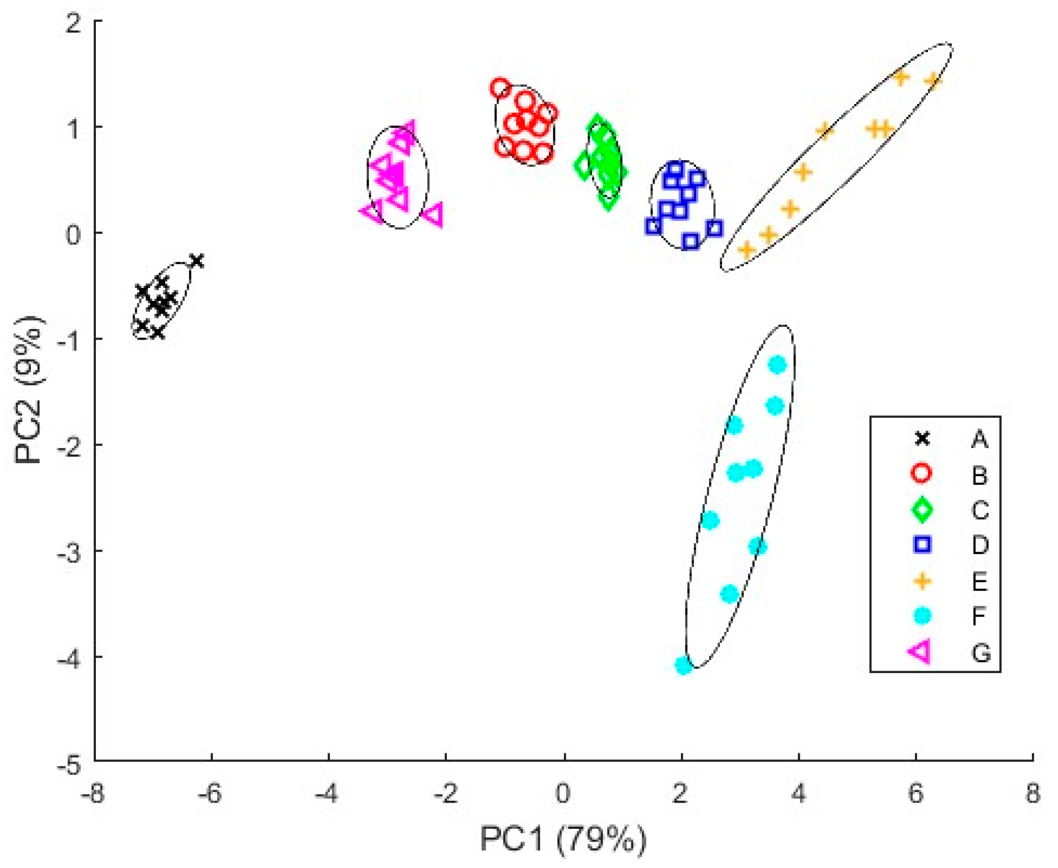
Figure 16.
PLS with MOX sensors only. (a) CH4 PLS, (b) CO2 PLS.
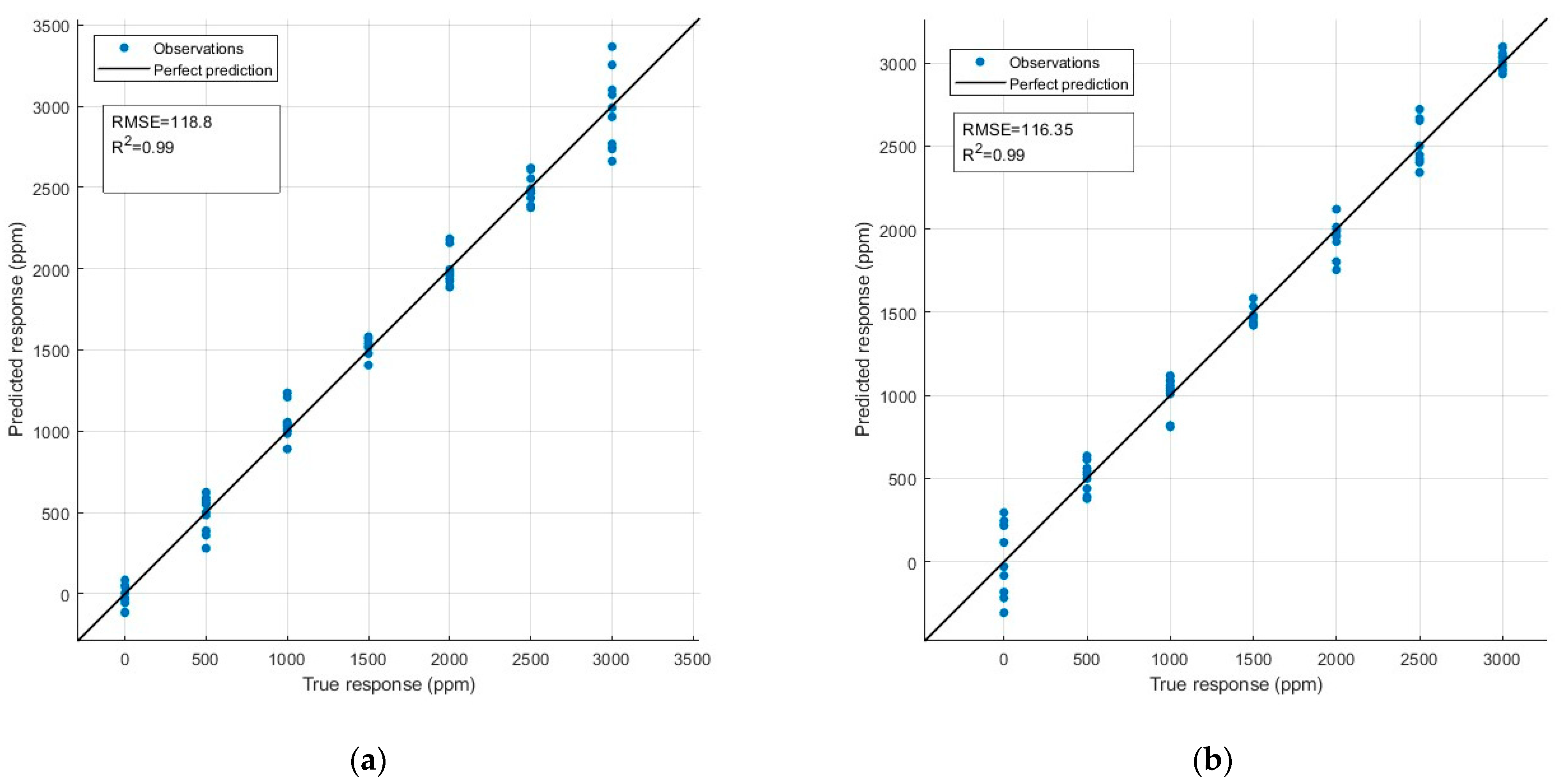
Figure 17.
PLS with MOX sensors and NDIR sensors. (a) CH4 PLS, (b) CO2 PLS.


Table 1.
Main board sensors and their measured signals.
| Sensor | Manufacturer | Type | Signals (Variables) |
|---|---|---|---|
| BME680 | Bosch | MOX | Temperature (S1), pressure (S2), relative humidity (S3), gas resistance (S4) |
| SGP30 | Sensirion | MOX | CO2 (S5), TVOC (S6), H2 (S7), Ethanol (S8) |
| CCS811 | ScioSense | MOX | CO2 (S9), TVOC (S10), gas resistance (S11) |
| ZMOD4410 | Renesas | MOX | Raw signal (S12), Ethanol (S13), TVOC (S14), CO2 (S15), air quality index (S16) |
| SGP40 | Sensirion | MOX | Gas resistance (S17) |
| SCD40 | Sensirion | NDIR | Temperature (S18), relative humidity (S19), CO2 (S20) |
| SHT21 | Sensirion | Temperature/relative humidity | Temperature (S21), relative humidity (S22) |
Table 2.
Secondary board sensors and their measured signals.
| Sensor | Manufacturer | Type | Signals (Variables) |
|---|---|---|---|
| IRC-A1 | Alphasense | CO2-NDIR | Reference signal (S23), active signal (S24), thermistor (S25) |
| IRC-AT | Alphasense | CO2-NDIR | Reference Signal (S26), active signal (S27), thermistor (S28) |
| IRM-AT | Alphasense | CH4-NDIR | Reference signal (S29), active signal (S30), thermistor (S31) |
| SJH-5 | GasLab | CH4-NDIR | Analog (S32), gas (S33) |
| MSH-P | Dynament | N2O-NDIR | Analog (S34), gas (S35) |
| IRNET-P-20 | Nenvitech | CH4-NDIR | Analog (S36), gas (S37) |
Table 3.
CH4 and CO2 mixture concentration.
| CH4 (ppm) | CO2 (ppm) |
|---|---|
| 3000 | 0 |
| 2500 | 500 |
| 2000 | 1000 |
| 1500 | 1500 |
| 1000 | 2000 |
| 500 | 2500 |
| 0 | 3000 |
Table 4.
Levels of air quality given with ZMOD4410.
| IAQ Rating | Air Information | Air Quality |
|---|---|---|
| ≤1.99 | Clean hygienic air | Very good |
| 2.0 to 2.99 | Good air quality (if no threshold value is exceeded) | Good |
| 3.00 to 3.99 | Noticeable comfort concerns (not recommended for exposure > 12 months) | Medium |
| 4.00 to 4.99 | Significant comfort issues (not recommended for exposure > 1 month | Poor |
| ≥5.0 | Unacceptable conditions (not recommended) | Bad |
Disclaimer/Publisher’s Note: The statements, opinions and data contained in all publications are solely those of the individual author(s) and contributor(s) and not of MDPI and/or the editor(s). MDPI and/or the editor(s) disclaim responsibility for any injury to people or property resulting from any ideas, methods, instructions or products referred to in the content. |
© 2023 by the authors. Licensee MDPI, Basel, Switzerland. This article is an open access article distributed under the terms and conditions of the Creative Commons Attribution (CC BY) license (https://creativecommons.org/licenses/by/4.0/).
Share and Cite
MDPI and ACS Style
González, V.; Meléndez, F.; Arroyo, P.; Godoy, J.; Díaz, F.; Suárez, J.I.; Lozano, J. Electro-Optical Nose for Indoor Air Quality Monitoring. Chemosensors 2023, 11, 535. https://doi.org/10.3390/chemosensors11100535
AMA Style
González V, Meléndez F, Arroyo P, Godoy J, Díaz F, Suárez JI, Lozano J. Electro-Optical Nose for Indoor Air Quality Monitoring. Chemosensors. 2023; 11(10):535. https://doi.org/10.3390/chemosensors11100535
Chicago/Turabian StyleGonzález, Víctor, Félix Meléndez, Patricia Arroyo, Javier Godoy, Fernando Díaz, José Ignacio Suárez, and Jesús Lozano. 2023. "Electro-Optical Nose for Indoor Air Quality Monitoring" Chemosensors 11, no. 10: 535. https://doi.org/10.3390/chemosensors11100535
Note that from the first issue of 2016, this journal uses article numbers instead of page numbers. See further details here.