On a New Discrete SEIADR Model with Mixed Controls: Study of Its Properties

Abstract

A new discrete SEIADR epidemic model is built based on previous continuous models. The model considers two extra subpopulation, namely, asymptomatic and lying corpses on the usual SEIR models. It can be of potential interest for diseases where infected corpses are infectious like, for instance, Ebola. The model includes two types of vaccinations, a constant one and another proportional to the susceptible subpopulation, as well as a treatment control applied to the infected subpopulation. We study the positivity of the controlled model and the stability of the equilibrium points. Simulations are made in order to provide allocation and examples to the different possible conditions. The equilibrium point with no infection and its stability is related, via the reproduction number values, to the reachability of the endemic equilibrium point.

1. Introduction

We present an SEIADR epidemic model (Susceptible-Exposed-symptomatic Infectious- Asymptomatic Infectious- Dead infected-Recovered) based on typical descriptions of the spread of an infectious disease made in the background literature [1,2,3,4,5,6]. We will adapt the continuous time model from previous papers, such as [7], into a discrete model. We incorporate two subpopulations, namely, asymptomatic and dead infective corpses to the SEIR module. In this way, the model can be useful for diseases where the lying corpses are infective like, for example, Ebola virus disease, with eventual asymptomatic infectious. Our motivations for the discretization are an improvement in the manipulation of the dynamic equations and a major control in the adjustments of the sampling period, which will facilitate the adaptation of the model into a real situation, which this work is ultimately aimed at. The model has four types of infected subpopulations so that each of the possible stages of the disease is characterized by a different subpopulation. This makes the model interesting for its application for studies in the Ebola disease and similar diseases in which the re-emergences of the presence of infectious individuals cannot be explained otherwise [8]. The infected stage of the alive population is split into three different subpopulations, namely, the exposed, the symptomatic infectious and the asymptomatic infectious subpopulation, where an individual may be contagious even if he/she/it does not show the symptoms of the disease [9,10]. Furthermore, we have designed our model in order to take into account the deceased infectious individuals as a new infectious subpopulation, so we can prove their importance in dynamics of the population as the contagiousness is still present on some of the corpses, that must be disposed with great care [9,11,12,13]. Thus, the final stages of the illness under study can be split into live and immune individuals, i.e., recovered (R) subpopulation, and infectious and dead individuals, i.e., dead (D) subpopulation. Given this, it has been widely studied the non negativity of the solutions [14,15,16] and the use of perturbations and nonlinear incidence rates (as seen in [17,18,19] and [19,20,21,22], respectively). Reducing the disease within the population should be main objective of the control measures proposed i.e., vaccination strategies and the medical treatment of the infectious subpopulation through antiviral treatment or care of the symptoms, which we will also include in our equations. This type of control strategies have been proposed in many models in the literature [3,9,14,15,23,24,25,26,27]. The stability analysis and control optimization of a a subpopulation of infectious individuals in treatment with vaccination is addressed in [28], and a time-delay model with a strategy of impulsive vaccination and a saturated incidence rate is addressed in [29]. For both the continuous and the discrete-time dynamic system with closed-loop stabilizing controllers, the properties of convergence of the state-trajectory to the equilibrium points and their global stability are very important tools for analyzing and designing those models. See, for instance [30,31,32,33], and some of the references therein. Therefore, we pay special attention to those properties in the proposed and studied controlled discrete epidemic model subject to a feedback vaccination control applied on the susceptible and to a feedback control on the infected subpopulation and to the relevance of the reproduction number, linked to the controller gains in the rates of convergence. Another relevant pillar of the study performed in this paper is the relevance of the discretization concerned to the positivity of the solution sequences and the attainability or un-attainability of the endemic equilibrium point depending on the value of the reproduction number. On the other hand, and concerned with the advantages statement of discrete epidemic models, we might point out that the performance of their continuous-time counterparts can be essentially kept if the discretization process is performed with good adjustments of the sampling period and the auxiliary discretization parameters in such a discrete-model. In particular, the computing time and the computer memory storage needs for control implementation can be reduced. A discrete epidemic model has been proposed, analyzed and discussed in [34] involving two interacting populations, the vector and the avian populations. The stability analysis and the stability properties of the equilibrium points of a pair of SIRS models subject to two viruses has been performed in [35]. Also, an important computational work has been implemented to illustrate the validity of the obtained results. On the other hand, the design of the stabilizing controllers have been recently invoked and developed with a well-worked mathematical rigor in [36,37], respectively. Finally, a study of the nonlinear phenomena of bifurcation and chaos has been detailed in [38] for a discrete SI epidemic model with fractional order while [39] gives a relevance of the fractional framework to the statement of fractional-type discrete epidemic models especially through the list of commented listed “ad hoc” references. In this paper, a discrete SEIADR model is proposed as a more generic variant of the SEIR one. A multiple set of possible control parameters is proposed, and all the different possible predictions about the population dynamics are studied through simulations in order to confirm the performed study.

The main novelties of this paper are:

• The characterization of the relations between the stability of the disease free equilibrium (DFE) point and the reachability of the endemic (END) one for the discrete SEIADR model under positive conditions.
• The study of the stability and positivity properties and the equilibrium points and their properties.
• The study through numerical examples of the influence of the controller gain in the equilibrium points and in the rates of convergence even under a similar reproduction number.

The paper is organized as follows. Section 2 describes the SEIADR model with vaccination campaigns and antiviral treatments. A study of the disease free and the endemic equilibrium points is made. The discretization of the continuous model and the conditions for the positivity of the subpopulations are described in detail in Section 3. Section 4 gives and discusses the stability of the equilibrium points of this discrete model through the use of the next generation matrix applied to the disease free equilibrium point. Some results of simulations of the dynamics with a reproduction number above and under one are presented at Section 5. Conclusions based on these results are presented in Section 6.

2. The Continuous SEIADR Model

The dynamics of the SEIADR model is defined by the following equations:

$$\mathrm{S}\left(t\right)=b_1-V+\eta \mathrm{R}\left(t\right)-\mathrm{S}\left(t\right)\left(\frac{\beta \mathrm{I}\left(t\right)+{\beta }_{\mathrm{A}}\mathrm{A}\left(t\right)+{\beta }_{\mathrm{D}}\mathrm{D}\left(t\right)}{N\left(t\right)}+b_2+K_V\right),$$

(1)

$$\mathrm{E}\left(t\right)=\mathrm{S}\left(t\right)\left(\frac{\beta \mathrm{I}\left(t\right)+{\beta }_{\mathrm{A}}\mathrm{A}\left(t\right)+{\beta }_{\mathrm{D}}\mathrm{D}\left(t\right)}{N\left(t\right)}\right)-(b_2+\gamma )\mathrm{E}\left(t\right),$$

(2)

$$\mathrm{I}\left(t\right)=p\gamma \mathrm{E}-(b_2+{\tau }_0+K_{\xi }+\alpha )\mathrm{I}\left(t\right),$$

(3)

$$\mathrm{A}\left(t\right)=(1-p)\gamma \mathrm{E}-(b_2+{\tau }_0)\mathrm{A}\left(t\right),$$

(4)

$$\mathrm{D}\left(t\right)=\alpha \mathrm{I}\left(t\right)+(\mathrm{I}\left(t\right)+\mathrm{A}\left(t\right))b_2-\mu \mathrm{D}\left(t\right),$$

(5)

$$\mathrm{R}\left(t\right)=V+K_{\xi }\mathrm{I}\left(t\right)+K_V\mathrm{S}\left(t\right)+{\tau }_0(\mathrm{A}\left(t\right)+\mathrm{I}\left(t\right))-(b_2+\eta )\mathrm{R}\left(t\right),$$

(6)

with $N\left(t\right)=\mathrm{S}\left(t\right)+\mathrm{E}\left(t\right)+\mathrm{I}\left(t\right)+\mathrm{A}\left(t\right)+\mathrm{D}\left(t\right)+\mathrm{R}\left(t\right)$ being the total population, where S, E, I, A, D and R are the Susceptible, Exposed, Symptomatic Infectious, Asymptomatic Infectious, Dead Infectious corpses and Recovered subpopulations respectively. See [7] for a discussion of the continuous-time model. The parameters of the model are:

• $b_1$ is the recruitment/birth rate,
• $b_2$ is the natural average death rate,
• $\beta ,{\beta }_{\mathrm{A}},{\beta }_{\mathrm{D}}$ are the disease transmission coefficients from the susceptible to the symptomatic and asymptomatic infectious, and to the infective corpses subpopulations, respectively,
• $1/\eta$ is the average duration of the immunity period which reflects a transition state from the recovered to the susceptible,
• $\gamma$ is the transition rate from the exposed to the symptomatic and asymptomatic infectious,
• $\alpha$ is the extra average mortality being associated with the disease which affects to the symptomatic infectious subpopulation,
• ${\tau }_0$ is the natural recovery rate for the whole infectious subpopulation (i.e., A + I ),
• p is the exposed subpopulation fraction which becomes symptomatic infectious,
• 1−p is the exposed subpopulation fraction which becomes asymptomatic infectious,
• 1/$\mu$ is the average time of infectiousness after death,
• V, $K_V$ and $K_{\xi }$ are the constant vaccination gain, the proportional vaccination control gain and the antiviral treatment control gain respectively. The constant vaccination is bounded such that $V\in [0,b_1]$, so a fraction $V/b_1\in [0,1]$ of the new individuals of the system (newborn, immigrants) is vaccinated.

Remark 1.

We define a set of auxiliary parameters to be then used as follows: $B_E=b_2+\gamma$, $B_I=b_2+{\tau }_0+K_{\xi }+\alpha$, $B_A=b_2+{\tau }_0$, $B_R=b_2+\eta$, $f=\frac{\gamma p}{B_I},$ $f_A=\frac{\gamma (1-p)}{B_A},$ $f_D=f_A\frac{b_2}{\mu }+f\frac{b_2+\alpha }{\mu },$ $G_1=B_R+B_E-b_2+\mu f_D\frac{B_R-b_2}{b_2}$, $F=f\beta +f_A{\beta }_A+f_D{\beta }_D$ and $G_2=(B_R+K_V)(b_2{f}_D-\alpha f)$.

After using these auxiliary parameters in the Equations (1)–(6) the resulting equilibrium points of the solutions are:

• A disease-free equilibrium point given by $({\mathrm{S}}_{\mathrm{DFE}},0,0,0,0,{\mathrm{R}}_{\mathrm{DFE}})$ where

  $$\begin{array}{c}\hfill {\mathrm{S}}_{\mathrm{DFE}}=\frac{B_{\mathrm{R}}{N}_{\mathrm{DFE}}-V}{B_{\mathrm{R}}+K_V},{\mathrm{R}}_{\mathrm{DFE}}=\frac{K_V{N}_{\mathrm{DFE}}+V}{B_{\mathrm{R}}+K_V}\end{array}$$

  (7)

  with the total population at this point defined as $N_{\mathrm{DFE}}=\frac{b_1}{b_2}$.
• An endemic one given by $({\mathrm{S}}_{\mathrm{END}},{\mathrm{E}}_{\mathrm{END}},{\mathrm{I}}_{\mathrm{END}},{\mathrm{A}}_{\mathrm{END}},{\mathrm{D}}_{\mathrm{END}},{\mathrm{R}}_{\mathrm{END}})$ where:

  $$\begin{array}{c}\hfill {\mathrm{S}}_{\mathrm{END}}=B_{\mathrm{E}}\frac{G_2{\mathrm{S}}_{\mathrm{DFE}}+b_2{G}_1{N}_{\mathrm{DFE}}}{G_2{B}_{\mathrm{E}}+b_{2}F{G}_1},{\mathrm{E}}_{\mathrm{END}}=\frac{({\mathrm{S}}_{\mathrm{DFE}}-{\mathrm{S}}_{\mathrm{END}})(B_{\mathrm{R}}+K_V)}{G_1},\\ \hfill \\ \hfill {\mathrm{I}}_{\mathrm{END}}=f{\mathrm{E}}_{\mathrm{END}},{\mathrm{A}}_{\mathrm{END}}=f_{\mathrm{A}}{\mathrm{E}}_{\mathrm{END}},{\mathrm{D}}_{\mathrm{END}}=f_{\mathrm{D}}{\mathrm{E}}_{\mathrm{END}},\\ \hfill \\ \hfill {\mathrm{R}}_{\mathrm{END}}={\mathrm{R}}_{\mathrm{DFE}}+\frac{({\mathrm{S}}_{\mathrm{DFE}}-{\mathrm{S}}_{\mathrm{END}})(B_{\mathrm{E}}-(b_2+\mu f_{\mathrm{D}}(1+K_V/b_2)))}{G_1},\end{array}$$

  (8)

  with the total population at this point given by:

  $$\begin{array}{c}\hfill N_{\mathrm{END}}={\mathrm{S}}_{\mathrm{END}}+{\mathrm{E}}_{\mathrm{END}}+{\mathrm{I}}_{\mathrm{END}}+{\mathrm{A}}_{\mathrm{END}}+{\mathrm{D}}_{\mathrm{END}}+{\mathrm{R}}_{\mathrm{END}}=\frac{{\mathrm{S}}_{\mathrm{END}}F}{B_{\mathrm{E}}}.\end{array}$$

3. Discretization of the SEIADR

In some epidemic models, the vaccination and treatment control actions can be exerted with feedback information of the subpopulations, commonly the susceptible and infectious as the one presented in this paper. Since amounts of data on the subpopulation levels and parametrical computations to exert the controls through time have to be processed and monitored, the use of computer-controlled actions may be necessary. Generally speaking, the discretization of dynamic systems offers several potential computational advantages towards the controller synthesis, namely:

• Normally feedback control actions are exerted by discrete-time controllers, especially, if the volume of data to be processed is relevant since the computational load has to be supported by a computer. Therefore, it can be preferred to start with a discrete-time model of the process, which then generates discrete sequences of measurable data, than a continuous-time one since then discrete control sequences are directly generated by processing the available sequence of discrete measurable data. Note also that the discretization of a continuous-time model towards the use of a computer for taking actions is always an approximation of the continuous time-model. However the sampling period of a discrete-time model is a design parameter, which does not imply an approximation when running the model.
• It could be argued that in fact the use of a continuous-time model can be used for control generations through a computer but, in this case, the discretization period has to be very small in order to consider approximately valid the continuous-time control generation from continuous-time data. That is, there is no freedom to select the discretization sampling period. Note that if a discrete controller is accommodated to a discrete-time model then there is an important freedom in the choice of the sampling period, which takes the role of an extra control parameter which can be eventually time-varying, if it is compatible with the stability and bandwidth.
• There is an important saving in data memory storage needs when implementing control actions, since only a discretized sequence of measurements needs to be stored and the control actions can be exerted along a set of time instants while the computer can exert alternative monitoring or computation actions. Thus, the computing time for control implementation is reduced.

So, the use of a discrete-time feedback controller being accommodated to a discrete-time model does offer relevant advantages over related to a fast discretization of a closed-loop tandem of continuous-time and controller configuration in order to make an “ad hoc” computational control implementation. A discrete SEIADR model is formulated based on previous examples, as those of [34,39,40], i.e., on the approximation of the subsequent derivative of the vector $\mathbf{x}\left(t\right)=\left(\mathrm{S}\left(t\right),\mathrm{E}\left(t\right),\mathrm{I}\left(t\right),\mathrm{A}\left(t\right),\mathrm{D}\left(t\right),\mathrm{R}\left(t\right)\right)$

$$\begin{array}{c}\hfill \dot{\mathbf{x}}\left(t\right)\to \frac{\mathbf{x}(t+T)-\mathbf{x}(t-T)}{2T}+a(\mathbf{x}(t+T)-2x\left(t\right)+\mathbf{x}(t-T))\end{array}$$

(9)

where ${\mathbf{x}}_k$ is defined as ${\mathbf{x}}_k=\mathbf{x}\left(kT\right)$ so that the derivatives at the moments ${\mathbf{x}}_k$ is implemented in the equation:

$${\dot{\mathbf{x}}}_k=\frac{{\mathbf{x}}_k(1+2aT)-4aT{\mathbf{x}}_k-{\mathbf{x}}_k(1-2aT)}{2T}$$

The parameters “a” and T are real positive constants, being T the sampling period that we choose in order to adjust our model as desired, and “a” a modulating parameter introduced in order to guarantee the system’s positivity further described later on Proposition 1. Thus, the discrete equations result to be

$$\begin{array}{cc}{\mathrm{S}}_{k+1}=\hfill & \frac{2T}{1+2aT}\left(\left(2a-b_2+K_V+\frac{\beta {\mathrm{I}}_k+{\beta }_{\mathrm{A}}{\mathrm{A}}_k+{\beta }_{\mathrm{D}}{\mathrm{D}}_k}{N_k}\right){\mathrm{S}}_k+b_1-V+\eta {\mathrm{R}}_k\right)\hfill \\ \hfill & +\left(\frac{1-2aT}{1+2aT}\right){\mathrm{S}}_{k-1},\hfill \end{array}$$

(10)

$$\begin{array}{cc}{\mathrm{E}}_{k+1}\hfill & =\frac{2T}{1+2aT}\left((\beta {\mathrm{I}}_k+{\beta }_{\mathrm{A}}{\mathrm{A}}_k+{\beta }_{\mathrm{D}}{\mathrm{D}}_k)\frac{{\mathrm{S}}_k}{N_k}+(2a-B_{\mathrm{E}}){\mathrm{E}}_k\right)+\left(\frac{1-2aT}{1+2aT}\right){\mathrm{E}}_{k-1},\hfill \end{array}$$

(11)

$$\begin{array}{cc}{\mathrm{I}}_{k+1}\hfill & =\frac{2T}{1+2aT}\left(\gamma p{\mathrm{E}}_k+(2a-B_{\mathrm{I}}){\mathrm{I}}_k\right)+\left(\frac{1-2aT}{1+2aT}\right){\mathrm{I}}_{k-1},\hfill \end{array}$$

(12)

$$\begin{array}{cc}{\mathrm{A}}_{k+1}\hfill & =\frac{2T}{1+2aT}\left(\gamma (1-p){\mathrm{E}}_k+(2a-B_{\mathrm{A}}){\mathrm{A}}_k\right)+\left(\frac{1-2aT}{1+2aT}\right){\mathrm{A}}_{k-1},\hfill \end{array}$$

(13)

$$\begin{array}{cc}{\mathrm{D}}_{k+1}\hfill & =\frac{2T}{1+2aT}\left(b_2{\mathrm{A}}_k+(b_2+\alpha ){\mathrm{I}}_k+(2a-\mu ){\mathrm{D}}_k\right)+\left(\frac{1-2aT}{1+2aT}\right){\mathrm{D}}_{k-1},\hfill \end{array}$$

(14)

$$\begin{array}{cc}{\mathrm{R}}_{k+1}\hfill & =\frac{2T}{1+2aT}\left(V+K_V{\mathrm{S}}_k+{\tau }_0({\mathrm{A}}_k+{\mathrm{I}}_k)+K_{\xi }{\mathrm{I}}_k+(2a-B_{\mathrm{R}}){\mathrm{R}}_k\right)+\left(\frac{1-2aT}{1+2aT}\right){\mathrm{R}}_{k-1},\hfill \end{array}$$

(15)

Positivity of the Solution

In this section, we will prove that the subpopulations affected by the disease always remain non-negative, provided that the initial condition is non-negative. The parameter “a” will be used to tune the discrete model so that its positivity is guaranteed. In the following, the notation for a vector $\mathbf{x}\ge 0$ means that all its components are non negative. We refer to a model with nonnegative solutions as a positive system.

Proposition 1.

Assume that $b_1\ge V$ and that for any $k\ge 1$, ${\mathit{x}}_k\ge 0$, ${\mathit{x}}_{k-1}\ge 0$

$$\frac{1}{2T}>a>\frac{1}{2}max\left[B_E,B_I,B_R,\mu ,max\left[\beta ,{\beta }_A,{\beta }_D\right]+b_2+K_V\right]$$

(16)

for which a necessary condition is $T\le \frac{1}{\left[B_E,B_I,B_R,\mu ,max\left[\beta ,{\beta }_A,{\beta }_D\right]+b_2+K_V\right]}$. Then ${\mathit{x}}_{k+1}\ge 0$. As a consequence, if ${\mathit{x}}_0\ge 0$ and ${\mathit{x}}_{-1}\ge 0$ then ${\mathit{x}}_k\ge 0;\forall k\ge 0$.

Proof. 

Assume that ${\mathbf{x}}_k=({\mathrm{S}}_k,{\mathrm{E}}_k,{\mathrm{I}}_k,{\mathrm{A}}_k,{\mathrm{D}}_k,{\mathrm{R}}_k)\ge 0$. Then, from the discrete dynamic Equations (10)–(15) the positivity for the values of ${\mathbf{x}}_{k+1}$ $=({\mathrm{S}}_{k+1},{\mathrm{E}}_{k+1},$ ${\mathrm{I}}_{k+1},$ ${\mathrm{A}}_{k+1},{\mathrm{D}}_{k+1}$ $,{\mathrm{R}}_{k+1})$ is studied as:

$$\begin{array}{ccc}\hfill {\mathrm{S}}_{k+1}& \ge & \frac{2T}{1+2aT}\left(2a-(b_2+K_V)-\frac{(\beta {\mathrm{I}}_k+{\beta }_{\mathrm{A}}{\mathrm{A}}_k+{\beta }_{\mathrm{D}}{\mathrm{D}}_k)}{N_k}\right){\mathrm{S}}_k\hfill \end{array}$$

(17)

$$\begin{array}{cc}=& \frac{2T}{1+2aT}\left(2a-(b_2+K_V)-(\beta n_i+{\beta }_{\mathrm{A}}{n}_a+{\beta }_{\mathrm{D}}{n}_d)\right){\mathrm{S}}_k\hfill \end{array}$$

(18)

$$\begin{array}{cc}\ge & \frac{2T}{1+2aT}\left(2a-\left(b_2+K_V+max[\beta ,{\beta }_{\mathrm{A}},{\beta }_{\mathrm{D}}]\right)\right){\mathrm{S}}_k\ge 0,\hfill \end{array}$$

(19)

Since $\frac{\mathrm{I}}{N}+\frac{\mathrm{A}}{N}+\frac{\mathrm{D}}{N}=n_i+n_a+n_d\le 1$. Also

$$\begin{array}{ccc}\hfill {\mathrm{E}}_{k+1}& \ge & \frac{2T}{1+2aT}\left(2a-B_{\mathrm{E}}\right){\mathrm{E}}_k\ge 0,\hfill \end{array}$$

(20)

$$\begin{array}{ccc}\hfill {\mathrm{I}}_{k+1}& \ge & \frac{2T}{1+2aT}\left(2a-B_{\mathrm{I}}\right){\mathrm{I}}_k\ge 0,\hfill \end{array}$$

(21)

$$\begin{array}{ccc}\hfill {\mathrm{A}}_{k+1}& \ge & \frac{2T}{1+2aT}\left(2a-B_{\mathrm{A}}\right){\mathrm{A}}_k\ge 0,\hfill \end{array}$$

(22)

$$\begin{array}{ccc}\hfill {\mathrm{D}}_{k+1}& \ge & \frac{2T}{1+2aT}\left(2a-\mu \right){\mathrm{D}}_k\ge 0,\hfill \end{array}$$

(23)

$$\begin{array}{ccc}\hfill {\mathrm{R}}_{k+1}& \ge & \frac{2T}{1+2aT}\left(2a-B_{\mathrm{R}}\right){\mathrm{R}}_k\ge 0.\hfill \end{array}$$

(24)

So ${\mathbf{x}}_{k+1}=({\mathrm{S}}_{k+1},{\mathrm{E}}_{k+1},{\mathrm{I}}_{k+1},{\mathrm{A}}_{k+1},{\mathrm{D}}_{k+1},{\mathrm{R}}_{k+1})$ is non negative provided that ${\mathbf{x}}_k\ge 0$. As a result via compute induction if ${\mathbf{x}}_0\ge 0$ and ${\mathbf{x}}_{-1}\ge 0$ then ${\mathbf{x}}_k\ge 0$, $\forall k\ge 0$. □

Remark 2.

Note that the modulating discretization parameter $“a”$ can grow at most linearly with the half of the inverse of the sampling period. As a result of proposition, if ${\mathit{x}}_0\ge 0$ and ${\mathit{x}}_{-1}=0$ then ${\mathit{x}}_k\ge 0\forall k\ge 0$.

4. Equilibrium Points: Positivity and Stability

From the discrete dynamic Equations (10)–(15), we calculate the equilibrium points such that ${\mathbf{x}}_{k+1}={\mathbf{x}}_k={\mathbf{x}}_{k-1}$ leading to:

$$\begin{array}{cc}\hfill {\mathrm{S}}^{*}& =\frac{2T}{1+2aT}\left(-\left(b_2+K_V+\frac{(\beta {\mathrm{I}}^{*}+{\beta }_{\mathrm{A}}{\mathrm{A}}^{*}+{\beta }_{\mathrm{D}}{\mathrm{D}}^{*})}{N^{*}}\right){\mathrm{S}}^{*}+b_1-V+\eta {\mathrm{R}}^{*}+\frac{1+2aT}{2T}{\mathrm{S}}^{*}\right),\hfill \end{array}$$

(25)

$$\begin{array}{cc}\hfill {\mathrm{E}}^{*}& =\frac{2T}{1+2aT}\left((\beta {\mathrm{I}}^{*}+{\beta }_{\mathrm{A}}{\mathrm{A}}^{*}+{\beta }_{\mathrm{D}}{\mathrm{D}}^{*})\frac{{\mathrm{S}}^{*}}{N^{*}}+\left(\frac{1+2aT}{2T}-B_{\mathrm{E}}\right){\mathrm{E}}^{*}\right),\hfill \end{array}$$

(26)

$$\begin{array}{cc}\hfill {\mathrm{I}}^{*}& =\frac{2T}{1+2aT}\left(\gamma p{\mathrm{E}}^{*}+\left(\frac{1+2aT}{2T}-B_{\mathrm{I}}\right){\mathrm{I}}^{*}\right),\hfill \end{array}$$

(27)

$$\begin{array}{cc}\hfill {\mathrm{A}}^{*}& =\frac{2T}{1+2aT}\left(\gamma (1-p){\mathrm{E}}^{*}+\left(\frac{1+2aT}{2T}-B_{\mathrm{A}}\right){\mathrm{A}}^{*}\right),\hfill \end{array}$$

(28)

$$\begin{array}{cc}\hfill {\mathrm{D}}^{*}& =\frac{2T}{1+2aT}\left(b_2{\mathrm{A}}^{*}+\left(b_2+\alpha \right){\mathrm{I}}^{*}+\left(\frac{1+2aT}{2T}-\mu \right){\mathrm{D}}^{*}\right),\hfill \end{array}$$

(29)

$$\begin{array}{cc}\hfill {\mathrm{R}}^{*}& =\frac{2T}{1+2aT}\left(V+K_V{\mathrm{S}}^{*}+{\tau }_0({\mathrm{A}}^{*}+{\mathrm{I}}^{*})+K_{\xi }{\mathrm{I}}^{*}+\left(\frac{1+2aT}{2T}-B_{\mathrm{R}}\right){\mathrm{R}}^{*}\right).\hfill \end{array}$$

(30)

The resulting equilibrium points are equal to the continuous-time model counterpart. The disease free equilibrium point is defined as $({\mathrm{S}}_{\mathrm{DFE}},0,0,0,0,{\mathrm{R}}_{\mathrm{DFE}})$, with ${\mathrm{S}}_{\mathrm{DFE}}$ and ${\mathrm{R}}_{\mathrm{DFE}}$ defined as in Equation (7), while the endemic equilibrium point $({\mathrm{S}}_{\mathrm{END}},{\mathrm{E}}_{\mathrm{END}},$ ${\mathrm{I}}_{\mathrm{END}},{\mathrm{A}}_{\mathrm{END}},$ ${\mathrm{D}}_{\mathrm{END}},{\mathrm{R}}_{\mathrm{END}})$ is defined as in Equation (8). Observe that, from Proposition 1, for a non-negative initial state, the system remains positive, so if ${\mathrm{S}}_{\mathrm{DFE}}-{\mathrm{S}}_{\mathrm{END}}<0$ the values at the endemic equilibrium of the infectious subpopulations, defined in Equation (8), are negative. Therefore, the endemic equilibrium is not reachable.

4.1. Local Asymptotic Stability of the DFE Point

In this section, we will study the disease free equilibrium point (DFE) $x_{\mathrm{DFE}}$ and obtain the Reproduction number, which would reveal us if it is locally stable or unstable. The stability of the DFE point is studied by constructing the next generation matrix. First we define the vector ${\mathbf{y}}_k$ as

$${\mathbf{y}}_k=[{\mathrm{E}}_k,{\mathrm{I}}_k,{\mathrm{A}}_k,{\mathrm{D}}_k,{\mathrm{E}}_{k-1},{\mathrm{I}}_{k-1},{\mathrm{A}}_{k-1},{\mathrm{D}}_{k-1},{\mathrm{S}}_k,{\mathrm{R}}_k,{\mathrm{S}}_{k-1},{\mathrm{R}}_{k-1}]$$

and then linearize around the DFE point (${\mathbf{x}}_k={\mathbf{x}}_{k-1}={\mathbf{x}}_{\mathrm{DFE}}$), so we get the constant Jacobian matrix:

$$\begin{array}{ccc}\hfill \mathbf{J}& =& {\left.\frac{\partial {\mathbf{y}}_{k+1}}{\partial {\mathbf{y}}_k}\right|}_{x_{\mathrm{DFE}}}=\left(\begin{array}{cc}F-\Sigma & 0\\ \Delta & C\end{array}\right).\hfill \end{array}$$

We focus on the the 8 × 8 submatrix $F-\Sigma$, related to the infectious subpopulations E, I, A, and D, while F represents the appearance of new set of infections and $\Sigma$ would describe the transitions between those infectious subpopulations. Thus, we define F as

$$\begin{array}{c}\hfill F=\frac{2{\mathrm{S}}_{\mathrm{DFE}}T}{N_{\mathrm{DFE}}(1+2aT)}\left(\begin{array}{cccccccc}0& \beta & {\beta }_{\mathrm{A}}& {\beta }_{\mathrm{D}}& 0& 0& 0& 0\\ 0& 0& 0& 0& 0& 0& 0& 0\\ 0& 0& 0& 0& 0& 0& 0& 0\\ 0& 0& 0& 0& 0& 0& 0& 0\\ 0& 0& 0& 0& 0& 0& 0& 0\\ 0& 0& 0& 0& 0& 0& 0& 0\\ 0& 0& 0& 0& 0& 0& 0& 0\\ 0& 0& 0& 0& 0& 0& 0& 0\end{array}\right)\end{array}$$

and $\Sigma$ as

$$\begin{array}{c}\hfill \Sigma =\left(\begin{array}{cccccccc}\frac{2T(B_{\mathrm{E}}-2a)}{2aT+1}& 0& 0& 0& \frac{2aT-1}{2aT+1}& 0& 0& 0\\ \frac{-2Tp\gamma }{2aT+1}& \frac{2T(B_{\mathrm{I}}-2a)}{2aT+1}& 0& 0& 0& \frac{2aT-1}{2aT+1}& 0& 0\\ \frac{-2T(1-p)\gamma }{2aT+1}& 0& \frac{2T(B_{\mathrm{A}}-2a)}{2aT+1}& 0& 0& 0& \frac{2aT-1}{2aT+1}& 0\\ 0& \frac{-2T(b_2+\alpha )}{2aT+1}& \frac{-2T{b}_2}{2aT+1}& \frac{2T(\mu -2a)}{2aT+1}& 0& 0& 0& \frac{2aT-1}{2aT+1}\\ -1& 0& 0& 0& 0& 0& 0& 0\\ 0& -1& 0& 0& 0& 0& 0& 0\\ 0& 0& -1& 0& 0& 0& 0& 0\\ 0& 0& 0& -1& 0& 0& 0& 0\end{array}\right).\end{array}$$

The next generation matrix (NGM) will be defined as:

$$\begin{array}{c}F{(I+\Sigma )}^{-1}=\\ \left(\begin{array}{cccccccc}{a}_{11}& a_{12}& a_{13}& a_{14}& \frac{1-2aT}{1+2aT}{a}_{11}& \frac{1-2aT}{1+2aT}{a}_{12}& \frac{1-2aT}{1+2aT}{a}_{13}& \frac{1-2aT}{1+2aT}{a}_{14}\\ 0& 0& 0& 0& 0& 0& 0& 0\\ 0& 0& 0& 0& 0& 0& 0& 0\\ 0& 0& 0& 0& 0& 0& 0& 0\\ 0& 0& 0& 0& 0& 0& 0& 0\\ 0& 0& 0& 0& 0& 0& 0& 0\\ 0& 0& 0& 0& 0& 0& 0& 0\\ 0& 0& 0& 0& 0& 0& 0& 0\end{array}\right)\end{array}$$

with

$$\begin{array}{c}{a}_{11}=\frac{{\mathrm{S}}_{\mathrm{DFE}}}{N_{\mathrm{DFE}}}\frac{F}{B_{\mathrm{E}}},a_{12}=\frac{{\mathrm{S}}_{\mathrm{DFE}}}{N_{\mathrm{DFE}}}\frac{(\beta \mu +{\beta }_{\mathrm{D}}(b_2+\alpha ))}{B_{\mathrm{I}}},a_{13}=\frac{{\mathrm{S}}_{\mathrm{DFE}}}{N_{\mathrm{DFE}}}\frac{({\beta }_{\mathrm{A}}\mu +{\beta }_{\mathrm{D}}{b}_2)}{B_{\mathrm{A}}\mu },a_{14}=\frac{{\mathrm{S}}_{\mathrm{DFE}}}{N_{\mathrm{DFE}}}\frac{{\beta }_{\mathrm{D}}}{\mu },\end{array}$$

The spectral radius of the NGM, defined as the maximum of the absolute value of all possible eigenvalues of the NGM, $\rho (F{(I+\Sigma )}^{-1})$ will correspond to the reproduction number

$${\mathrm{R}}_0=\frac{{\mathrm{S}}_{\mathrm{DFE}}F}{N_{\mathrm{DFE}}{B}_{\mathrm{E}}}=\frac{{\mathrm{S}}_{\mathrm{DFE}}{N}_{\mathrm{END}}}{{\mathrm{S}}_{\mathrm{END}}{N}_{\mathrm{DFE}}}.$$

(31)

We have concluded from the above discussion the following result:

Theorem 1.

The DFE point is locally asymptotically stable if $R_0<1$, while if $R_0>1$, then the DFE point is unstable.

4.2. Conditions of Positivity of the Equilibrium Points

Here we will establish the conditions for the positivity, and thus, the potential reachability for any non-negative initial conditions, of the equilibrium points. Note that any non-negative solutions under Proposition 1 can reach an equilibrium point only if that has non-negative components.

4.2.1. DFE Point

The following result is direct:

Proposition 2.

$x_{\mathrm{DFE}}\ge 0$ if $V\le b_1(1+\mu /b_2)$.

Proof. 

Note that ${\mathrm{I}}_{\mathrm{DFE}}={\mathrm{A}}_{\mathrm{DFE}}={\mathrm{E}}_{\mathrm{DFE}}={\mathrm{D}}_{\mathrm{DFE}}=0$. Also note that ${\mathrm{S}}_{\mathrm{DFE}}\ge 0$ if $V\le b_1(1+\eta /b_2)$ from (7) and $N_{\mathrm{DFE}}=b_1/b_2>0$. Then, again from (7), ${\mathrm{R}}_{\mathrm{DFE}}\ge 0$. As a result, $x_{\mathrm{DFE}}\ge 0$. □

4.2.2. END Point

The positivity of the END point relies on the positivity of $\Delta \mathrm{S}=\left({\mathrm{S}}_{\mathrm{DFE}}-{\mathrm{S}}_{\mathrm{END}}\right)$ as it is seen in (8) to guarantee that ${\mathrm{E}}_{\mathrm{END}}\ge 0$. Let us define:

$$x\equiv -\frac{N_{\mathrm{DFE}}-N_{\mathrm{END}}}{{\mathrm{S}}_{\mathrm{DFE}}-{\mathrm{S}}_{\mathrm{END}}}=\frac{\Delta N}{\Delta \mathrm{S}}=\frac{G_2}{b_2{G}_1}.$$

It is direct to see that the reproduction number, defined in (31), can be equivalently written as

$${\mathrm{R}}_0(\Delta \mathrm{S},x)=(1+\frac{\Delta \mathrm{S}}{{\mathrm{S}}_{\mathrm{END}}})(1+x\frac{\Delta \mathrm{S}}{N_{\mathrm{DFE}}}),$$

(32)

so if $x\ge 0$, this implies that the reachability of the END point is given a reproduction number ${\mathrm{R}}_0>1$, as $\Delta \mathrm{S}>0\iff {\mathrm{R}}_0>1$, and $\Delta \mathrm{S}<0\iff {\mathrm{R}}_0<1$. The case $x=0$ is not relevant for the analysis.

Proposition 3.

The non negativity of x is guaranteed if $\mu <\frac{b_2^2{B}_I+b_2(\alpha \tau -b_2{K}_{\xi })p}{B_A\alpha p}$.

Proof. 

The parameter x can be written as $x=\frac{G_2}{b_2{G}_1}$, so that the positivity of $G_1$ is easily proven as

$$G_1=b_2+\eta +\gamma +\mu f_{\mathrm{D}}\eta /b_2>0$$

Thus $sign\left(G_2\right)=sign(b_2{f}_{\mathrm{D}}-\alpha f)=sign\left(\gamma \frac{b_2^2{B}_{\mathrm{I}}-p(B_{\mathrm{A}}\alpha \mu +b_2(b_2{K}_{\xi }-\tau \alpha ))}{B_{\mathrm{A}}{B}_{\mathrm{I}}\mu }\right)$, so

$$\begin{array}{c}\hfill \gamma \frac{b_2^2{B}_{\mathrm{I}}-p(B_{\mathrm{A}}\alpha \mu +b_2(b_2{K}_{\xi }-\tau \alpha ))}{B_{\mathrm{A}}{B}_{\mathrm{I}}\mu }>0,if\\ \hfill b_2^2{B}_{\mathrm{I}}-p(B_{\mathrm{A}}\alpha \mu +b_2(b_2{K}_{\xi }-\tau \alpha ))>0,\\ \hfill G_2>0if\mu <\frac{b_2^2{B}_{\mathrm{I}}+b_2(\alpha {\tau }_0-b_2{K}_{\xi })p}{B_{\mathrm{A}}\alpha p}.\end{array}$$

(33)

The subsequent result establishes that the existence of a reachable END point, which is defined by the positivity of x, will be also characterized by the reproduction number. □

Proposition 4.

If $b_2<\mu$, then the END point is reachable for any non-negative initial conditions if and only if $R_0\ge 1\iff \Delta S\ge 0$. If $R_0=1$ then the END point is coincident with the DFE one.

Proof. 

From (32), one gets:

$${\mathrm{R}}_0(\Delta \mathrm{S},x)=\frac{{\mathrm{S}}_{\mathrm{DFE}}(N_{\mathrm{DFE}}+x\Delta \mathrm{S})}{N_{\mathrm{DFE}}({\mathrm{S}}_{\mathrm{DFE}}-\Delta \mathrm{S})}.$$

(34)

We study first the solution for the critic value of the reproduction number ${\mathrm{R}}_0=1$. It follows from (32) that ${\mathrm{R}}_0=1$ if either $\Delta \mathrm{S}=0$ or $x=\frac{-N_{\mathrm{DFE}}}{{\mathrm{S}}_{\mathrm{DFE}}}$.

The derivative at the critic points will be

$$R_0^{\prime }(\Delta \mathrm{S},x)=\frac{d\left({\mathrm{R}}_0\right)}{d(\Delta \mathrm{S})}=\frac{{\mathrm{S}}_{\mathrm{DFE}}(N_{\mathrm{DFE}}+x{\mathrm{S}}_{\mathrm{DFE}})}{N_{\mathrm{DFE}}{({\mathrm{S}}_{\mathrm{DFE}}-\Delta \mathrm{S})}^2}$$

(35)

which gives us

• $R_0^{\prime }(\Delta \mathrm{S},-N_{\mathrm{DFE}}/{\mathrm{S}}_{\mathrm{DFE}})=0,\forall \Delta \mathrm{S}\in \mathbb{R}$, and
• for $x\ne -\frac{N_{\mathrm{DFE}}}{{\mathrm{S}}_{\mathrm{DFE}}}\Rightarrow R_0^{\prime }(\Delta \mathrm{S}=0,x)=\frac{1}{{\mathrm{S}}_{\mathrm{DFE}}}+\frac{x}{N_{\mathrm{DFE}}}$ so that if

  $$(x>-N_{\mathrm{DFE}}/{\mathrm{S}}_{\mathrm{DFE}}\iff R_0^{\prime }(\Delta \mathrm{S}=0,x)>0),$$

  then $\forall \Delta \mathrm{S}>0\Rightarrow {\mathrm{R}}_0>1$, since ${\mathrm{R}}_0(\Delta \mathrm{S},x)$ is non-decreasing with respect to $\Delta \mathrm{S}$ for all real $x>-\frac{N_{\mathrm{DFE}}}{{\mathrm{S}}_{\mathrm{DFE}}}$.

We know that x depends on the parameter p (i.e., the fraction of exposed which become symptomatic) as

$$\begin{array}{ccc}\hfill x=x\left(p\right)& =& \frac{G_2\left(p\right)}{b_2{G}_1\left(p\right)}\hfill \\ & =& \frac{\gamma \left(B_{\mathrm{R}}+K_V\right)\left(-p{B}_{\mathrm{A}}\left(b_2\left(\alpha +b_2\right)-\alpha \mu \right)+b_2^2{B}_{\mathrm{I}}(p-1)\right)}{b_2{B}_{\mathrm{I}}\gamma \eta \mu (p-1)-\mu B_{\mathrm{A}}\left(\gamma \eta p\left(\alpha +b_2\right)+b_2{B}_{\mathrm{I}}\left(b_2+\gamma +\eta \right)\right)},\hfill \end{array}$$

(36)

so that the derivative with respect to p is

$$\begin{array}{c}{x}^{\prime }\left(p\right)=\frac{dx\left(p\right)}{dp}=\left(\mu -b_2\right)\frac{\left(\alpha \gamma \eta +\alpha B_{\mathrm{A}}\left(b_2+\gamma +\eta \right)\right)}{\mu \left(B_P\right)}+\frac{b_2\left(\alpha \gamma \eta +b_2\left(b_2+\gamma +\eta \right)\left(\alpha +k_{\xi }\right)\right)}{\mu \left(B_P\right)}\end{array}$$

(37)

with

$$\begin{array}{c}{B}_P=\frac{{\left(b_2^2{B}_{\mathrm{A}}\left(\alpha +B_{\mathrm{A}}+k_{\xi }\right)+b_2\left(B_{\mathrm{A}}^2(\gamma +\eta )+B_{\mathrm{A}}\left(\eta (\alpha +\gamma )+\alpha \gamma +(\gamma +\eta )k_{\xi }\right)-\gamma \eta (p-1)\left(\alpha +k_{\xi }\right)\right)+\alpha \gamma \eta p{B}_{\mathrm{A}}\right)}^2}{b_2\gamma B_{\mathrm{A}}\left(b_2+\eta +K_V\right)\left(\alpha +B_{\mathrm{A}}+k_{\xi }\right)}>0.\end{array}$$

Since $\mu >b_2$, then $x^{\prime }\left(p\right)>0,\forall p\in [0,1]$, so the minimum value of $x\left(p\right)$ would be $x\left(0\right)$ and then:

$$x\left(p\right)\ge x\left(0\right)=\frac{-\gamma b_2(\eta +b_2+K_V)}{(b_2+\tau )(b_2+\eta +\gamma )\mu +\gamma \eta \mu }.$$

(38)

Thus, if

$$x\ge x\left(0\right)>-\frac{N_{\mathrm{DFE}}}{{\mathrm{S}}_{\mathrm{DFE}}},$$

(39)

(so that ${\mathrm{R}}_0(\Delta \mathrm{S},x)$ is non-decreasing with respect to $\Delta \mathrm{S}$) $\Rightarrow \Delta \mathrm{S}>0\iff {\mathrm{R}}_0>1$.

The inequality from (39) becomes through Equation (7):

$$\begin{array}{c}\hfill \frac{N_{\mathrm{DFE}}}{{\mathrm{S}}_{\mathrm{DFE}}}\ge \frac{b_2+\eta +K_V}{b_2+\eta }>-x\left(0\right)=\frac{(b_2+\eta +K_V)\gamma b_2/\mu }{\gamma \eta +(b_2+\tau )(b_2+\eta +\gamma )},\end{array}$$

(40)

which can be reduced to $1>{\displaystyle \frac{b_2/\mu }{1+\frac{\tau }{b_2+\tau }+\frac{B_{\mathrm{A}}}{\gamma }}}$, which is true if $b_2<\mu$.

On the other hand, the value of the susceptible subpopulation in the END point is defined from (8) as

$${\mathrm{S}}_{\mathrm{END}}=\frac{N_{\mathrm{DFE}}+x{\mathrm{S}}_{\mathrm{DFE}}}{F/B_{\mathrm{E}}+x}=\frac{(N_{\mathrm{DFE}}+x{\mathrm{S}}_{\mathrm{DFE}})}{({\mathrm{R}}_0+x{\mathrm{S}}_{\mathrm{DFE}}/N_{\mathrm{DFE}})N_{\mathrm{DFE}}/{\mathrm{S}}_{\mathrm{DFE}}},$$

(41)

which will be positive if $x>-N_{\mathrm{DFE}}/{\mathrm{S}}_{\mathrm{DFE}}$ and ${\mathrm{R}}_0\ge 1$. Note that for ${\mathrm{R}}_0=1$ the endemic equilibrium point is coincident with the DFE one since $\Delta \mathrm{S}=0$, so it is reachable. Then $R_0^{\prime }(\Delta \mathrm{S})>0$ and the existence of the END point is characterized by ${\mathrm{R}}_0\ge 1$. □

4.3. Global Stability

We know that the reproduction number of (31) can be rewritten as

$${\mathrm{R}}_0=\frac{b_2\gamma \left(b_1\left(\frac{\eta }{b_2}+1\right)-V\right)\left(\frac{p\left(\alpha +b_2\right){\beta }_{\mathrm{D}}+\beta \mu p}{\alpha +b_2+k_{\xi }+{\tau }_0}-\frac{(p-1)\left(\mu {\beta }_{\mathrm{S}}+b_2{\beta }_{\mathrm{D}}\right)}{b_2+{\tau }_0}\right)}{b_1\mu \left(b_2+\gamma \right)\left(b_2+\eta +K_V\right)}$$

(42)

and by using the relative disease transmission coefficients ${\beta }_{\mathrm{A}r}={\beta }_{\mathrm{A}}/\beta$ and ${\beta }_{\mathrm{D}r}={\beta }_{\mathrm{D}}/\beta$ we can rewrite the reproduction number as

$${\mathrm{R}}_0=\beta \frac{b_2\gamma \left(b_1\left(\frac{\eta }{b_2}+1\right)-V\right)\left(\frac{p\left(\alpha +b_2\right){\beta }_{\mathrm{D}r}+\mu p}{\alpha +b_2+k_{\xi }+{\tau }_0}-\frac{(p-1)\left(\mu {\beta }_{\mathrm{A}r}+b_2{\beta }_{\mathrm{D}r}\right)}{b_2+{\tau }_0}\right)}{b_1\mu \left(b_2+\gamma \right)\left(b_2+\eta +K_V\right)}.$$

(43)

Furthermore, the Jacobian matrix $\mathbf{J}$ on the equilibrium points is equal to

$$\mathbf{J}=\left(\begin{array}{cc}A& B\\ I_6& 0\end{array}\right)$$

(44)

with $B=\frac{1-2aT}{1+2aT}{I}_6$ and $A=\frac{2T}{1+2aT}Q$, being

$$Q=\left(\begin{array}{cccccc}{q}_{11}& q_{12}& q_{13}& q_{14}& q_{15}& q_{16}\\ q_{21}& q_{22}& q_{23}& q_{24}& q_{25}& q_{26}\\ 0& p\gamma & 2a-(b_2+{\tau }_0+k_{\xi }+\alpha )& 0& 0& 0\\ 0& \gamma -p\gamma & 0& 2a-(b_2+{\tau }_0)& 0& 0\\ 0& 0& \alpha +b_2& b_2& 2a-\mu & 0\\ K_V& 0& k_{\xi }+{\tau }_0& {\tau }_0& 0& 2a-\eta -b_2\end{array}\right),$$

with

$$\begin{array}{cc}{q}_{11}=2a-b_2-K_V-\frac{B_{\mathrm{E}}{\mathrm{E}}^{*}\left(N^{*}-{\mathrm{S}}^{*}\right)}{N^{*}{\mathrm{S}}^{*}}\hfill & q_{12}=\frac{B_{\mathrm{E}}{\mathrm{E}}^{*}}{N^{*}}\hfill \\ q_{13}=\frac{B_{\mathrm{E}}{\mathrm{E}}^{*}-\beta {\mathrm{S}}^{*}}{N^{*}}\hfill & q_{21}=B_{\mathrm{E}}{\mathrm{E}}^{*}\left(\frac{1}{{\mathrm{S}}^{*}}-\frac{1}{N^{*}}\right)\hfill \\ q_{22}=2a-\gamma -b_2-\frac{B_{\mathrm{E}}{\mathrm{E}}^{*}}{N^{*}}\hfill & q_{23}=\frac{\beta {\mathrm{S}}^{*}-B_{\mathrm{E}}{\mathrm{E}}^{*}}{N^{*}}\hfill \\ q_{14}=\frac{B_{\mathrm{E}}{\mathrm{E}}^{*}-{\mathrm{S}}^{*}{\beta }_{\mathrm{A}}}{N^{*}}\hfill & q_{15}=\frac{B_{\mathrm{E}}{\mathrm{E}}^{*}-{\mathrm{S}}^{*}{\beta }_{\mathrm{D}}}{N^{*}}\hfill \\ q_{16}=\eta +\frac{B_{\mathrm{E}}{\mathrm{E}}^{*}}{N^{*}}\hfill & q_{24}=\frac{{\beta }_{\mathrm{A}}{\mathrm{S}}^{*}-B_{\mathrm{E}}{\mathrm{E}}^{*}}{N^{*}}\hfill \\ q_{25}=\frac{{\beta }_{\mathrm{D}}{\mathrm{S}}^{*}-B_{\mathrm{E}}{\mathrm{E}}^{*}}{N^{*}}\hfill & q_{26}=-\frac{B_{\mathrm{E}}{\mathrm{E}}^{*}}{N^{*}}\hfill \end{array}$$

(45)

and $\{N^{*},{\mathrm{S}}^{*},{\mathrm{E}}^{*}\}\to \{N_{\mathrm{DFE}},{\mathrm{S}}_{\mathrm{DFE}},0\}$ for the Jacobian matrix associated to the DFE point ${\mathbf{J}}_{\mathrm{DFE}}$, and $\{N^{*},{\mathrm{S}}^{*},{\mathrm{E}}^{*}\}\to \{N_{\mathrm{END}},{\mathrm{S}}_{\mathrm{END}},{\mathrm{E}}_{\mathrm{END}}\}$ for the Jacobian matrix associated to the END point ${\mathbf{J}}_{\mathrm{END}}$. The matrix Q corresponding to ${\mathbf{J}}_{\mathrm{DEF}}$, namely, $Q_{\mathrm{DFE}}$ of the ${\mathbf{J}}_{\mathrm{DFE}}$ will then be equal to:

$$\begin{array}{c}\hfill Q_{\mathrm{DFE}}=\left(\begin{array}{ccccc}2a-b_2-K_V& 0& -\frac{\beta {\mathrm{S}}_{\mathrm{DFE}}}{N_{\mathrm{DFE}}}-\frac{{\beta }_{\mathrm{A}}{\mathrm{S}}_{\mathrm{DFE}}}{N_{\mathrm{DFE}}}& -\frac{{\beta }_{\mathrm{D}}{\mathrm{S}}_{\mathrm{DFE}}}{N_{\mathrm{DFE}}}& \eta \\ 0& 2a-\gamma -b_2& \frac{\beta {\mathrm{S}}_{\mathrm{DFE}}}{N_{\mathrm{DFE}}}\frac{{\beta }_{\mathrm{A}}{\mathrm{S}}_{\mathrm{DFE}}}{N_{\mathrm{DFE}}}& \frac{{\beta }_{\mathrm{D}}{\mathrm{S}}_{\mathrm{DFE}}}{N_{\mathrm{DFE}}}& 0\\ 0& p\gamma & 2a-(b_2+{\tau }_0+k_{\xi }+\alpha )& 0& 0\\ 0& (1-p)\gamma & 2a-(b_2+{\tau }_0)& 0& 0\\ 0& 0& \alpha +b_2{b}_2& 2a-\mu & 0\\ K_V& 0& k_{\xi }+{\tau }_0{\tau }_0& 0& 2a-(\eta +b_2)\end{array}\right)\end{array}$$

$$\begin{array}{c}\hfill Q_{\mathrm{DFE}}=2a{I}_6-\left(\begin{array}{ccccc}{b}_2+K_V& 0& \frac{\beta {\mathrm{S}}_{\mathrm{DFE}}}{N_{\mathrm{DFE}}}\frac{{\beta }_{\mathrm{A}}{\mathrm{S}}_{\mathrm{DFE}}}{N_{\mathrm{DFE}}}& \frac{{\beta }_{\mathrm{D}}{\mathrm{S}}_{\mathrm{DFE}}}{N_{\mathrm{DFE}}}& -\eta \\ 0& \gamma +b_2& -\frac{\beta {\mathrm{S}}_{\mathrm{DFE}}}{N_{\mathrm{DFE}}}-\frac{{\beta }_{\mathrm{A}}{\mathrm{S}}_{\mathrm{DFE}}}{N_{\mathrm{DFE}}}& -\frac{{\beta }_{\mathrm{D}}{\mathrm{S}}_{\mathrm{DFE}}}{N_{\mathrm{DFE}}}& 0\\ 0& -p\gamma & b_2+{\tau }_0+k_{\xi }+\alpha & 0& 0\\ 0& (p-1)\gamma & b_2+{\tau }_0& 0& 0\\ 0& 0& -\alpha -b_2-b_2& \mu & 0\\ -K_V& 0& -k_{\xi }-{\tau }_0-{\tau }_0& 0& \eta +b_2\end{array}\right)\end{array}$$

(46)

Assume that (16) hold. Then, the following result guarantees the global stability under positivity conditions of Proposition 1.

Theorem 2.

The following properties hold:

(i) 

The total population $N_k;\forall k\ge 0$ is positive and bounded for any given non-negative initial conditions.

(ii) 

The discrete SEIADR epidemic model is globally Lyapunov’s stable for any given finite non-negative initial conditions irrespective of the value of the reproduction number.

(iii) 

if ${\mathrm{R}}_0\le 1$ then the DFE point is the unique reachable equilibrium which is globally asymptotically stable.

Proof. 

Since $N_k={\mathrm{S}}_K+{\mathrm{E}}_K+{\mathrm{I}}_K+{\mathrm{A}}_K+{\mathrm{D}}_K+{\mathrm{R}}_K;\forall k\ge 0$, subject to any finite initial conditions satisfying $min({\mathrm{S}}_0,{\mathrm{E}}_0,{\mathrm{I}}_0,{\mathrm{A}}_0,{\mathrm{D}}_0,{\mathrm{R}}_0)\ge 0$, it turns out that $N_k\ge 0;\forall k\ge 0$ since all the subpopulations are non-negative for any sample from Proposition 1. Now, by summing up (10)–(15), one gets the following evolution equation for the total population:

$$N_{k+1}=\frac{1-2aT}{1+2aT}{N}_{k-1}+\frac{2T}{1+2aT}[2a{N}_k+b_1-\mu {\mathrm{D}}_K-b_2({\mathrm{E}}_K+{\mathrm{R}}_K+{\mathrm{S}}_K)];\forall k\ge 1$$

(47)

One gets from (47) that:

$${\widehat{N}}_{k+1}+\frac{2T\nu }{1+2aT}({\mathrm{D}}_K+{\mathrm{E}}_K+{\mathrm{R}}_K+{\mathrm{S}}_K)e_1⪯{\mathrm{A}}_N{\widehat{N}}_k+\frac{2T{b}_1}{1+2aT}{e}_1;\forall k\ge 1$$

(48)

where $\nu =min(b_2,\mu )$ and

$${\mathrm{A}}_N=\left(\begin{array}{cc}4aT/(1+2aT)& (1-2aT)/(1+2aT)\\ 1& 0\end{array}\right),$$

(49)

with ${\widehat{N}}_k={\left[N_k{N}_{k-1}\right]}^T;e_1={(1,0)}^T$ and the notation “⪯” in $M=\left(M_{ij}\right)⪯N=\left(N_{ij}\right)$ with M and N being of the same order means that $M_{ij}\le N_{ij};\forall i,j$, that is, the inequalities holds for all the corresponding matrix entries of M and N. It turns out by direct inspection that ${\mathrm{A}}_N$ is positive (in the sense that it has no negative entries) and convergent (i.e., stable in the discrete sense) since its eigenvalues are within the unity ratio circle in the complex plane. Now, assume that the sequence ${\{{\widehat{N}}_k\}}_{k=0}^{\infty }$ is unbounded to prove its boundedness by contradiction arguments. Then, it has a subsequence ${\{{\widehat{N}}_{k_n}\}}_{n=0}^{\infty }\subseteq {\{{\widehat{N}}_k\}}_{k=0}^{\infty }$ which is strictly increasing with ${\{k_n\}}_{n=0}^{\infty }$ being a strictly increasing sequence of non-negative integers, that is, ${\{{\widehat{N}}_{k_n}\}}_{n=0}^{\infty }\to \infty$ as $n\to \infty$ and one gets via recursive calculations from (48) and Proposition 1 that:

$$\begin{array}{c}\hfill 0⪯{\widehat{N}}_{k_{n+1}}+{\Sigma }_{i=k_n}^{k_{n+1}-1}{\left({\mathrm{A}}_N\right)}^{(k_{n+1}-(i+1))}({\mathrm{D}}_i+{\mathrm{E}}_i+{\mathrm{R}}_i+{\mathrm{S}}_i)e_1,\end{array}$$

(50)

$$\begin{array}{c}\hfill ⪯{\left({\mathrm{A}}_N\right)}^{(k_{n+1}-k_n)}{\widehat{N}}_{k_n}+{\Sigma }_{i=k_n}^{k_{n+1}-1}{\left({\mathrm{A}}_N\right)}^{(k_{n+1}-(i+1))}\frac{2T{b}_1}{1+2aT}{e}_1;\forall k\ge 1,\end{array}$$

(51)

since ${\mathrm{A}}_N$ is a convergent matrix so that spectral radius $r\left({\mathrm{A}}_N\right)=inf\parallel {\mathrm{A}}_N\parallel =\left|{\lambda }_{max}\left({\mathrm{A}}_N\right)\right|<1,{\mathrm{A}}_N\succ 0$ and ${\{{\widehat{N}}_{k_n}\}}_{n=0}^{\infty }$ is a non-negative strictly increasing sequence. Then one has from (51):

$$\begin{array}{c}\parallel {\widehat{N}}_{k_{n+m+1}}+{\Sigma }_{i=k_n}^{k_{n+m+1}-1}{\left({\mathrm{A}}_N\right)}^{(k_{n+m+1}-(i+1))}({\mathrm{D}}_i+{\mathrm{E}}_i+{\mathrm{R}}_i+{\mathrm{S}}_i)e_1\parallel \\ \le \parallel {\left({\mathrm{A}}_N\right)}^{(k_{n+m+1}-k_n)}{\widehat{N}}_{k_n}\parallel +\parallel {\Sigma }_{i=k_n}^{k_{n+m+1}-1}{\left({\mathrm{A}}_N\right)}^{(k_{n+m+1}-(i+1))}\frac{2T{b}_1}{1+2aT}{e}_1\parallel ;\forall k\ge 1\\ \le {\rho }^{k_{n+m-1}-k_n}\parallel {\widehat{N}}_{k_n}\parallel +\frac{2T{b}_1(1-{\rho }^{k_{n+m+1}-k_n})}{(1+2aT)\rho }\forall m\ge 0,\forall k\ge 1\end{array}$$

(52)

for some matrix norm $\parallel •\parallel$ such that $\parallel {\mathrm{A}}_N\parallel \le \rho =r\left({\mathrm{A}}_N\right)+ϵ<1$ for some given real constant $ϵ$ fulfilling $0\le ϵ<1-r\left({\mathrm{A}}_N\right)$. From the definition of the spectral radius and the fact that ${\mathrm{A}}_N$ is convergent such a norm upper-bounded by such a $\rho$ parameter always exists. By talking limits in (52) as $n,m\to \infty$, so that $(k_{n+m+1}-k_n)\to \infty$, one gets the contradiction $+\infty \le \frac{2T{b}_1}{(1+2aT)\rho }$. This happens since ${\widehat{N}}_{k_{n+m+1}}\to +\infty$ as $(n+m)\to \infty$ by the unboundedness assumption on $N_k$ as $k\to \infty$ and $\rho <1,{\mathrm{D}}_K+{\mathrm{E}}_K+{\mathrm{R}}_K+{\mathrm{S}}_K\ge 0$ and $N_k\ge 0$; $\forall k\ge 0$ from the non-negativity of the subpopulations with the conditions of Proposition 1. Then, $N_k;\forall k\ge 0$ is bounded for any given non-negative initial conditions and Property (i) follows. Property (ii) is a direct consequence of Property (i) and the non-negativity of all the subpopulations for any sample and given finite non-negative initial conditions. Property (iii) follows since if ${\mathrm{R}}_0<1$ the END point is not reachable and if ${\mathrm{R}}_0=1$ it is coincident with the DFE one. Therefore for ${\mathrm{R}}_0\le 1$ the unique reachable equilibrium point from non-negative initial conditions is the DFE one which is globally asymptotically stable since it is locally asymptotically stable from Theorem 1. □

5. Numerical Simulations

We start the simulation with the subpopulations in an initial conditions next to the DFE point, concretely:

$$(\mathrm{S}\left(0\right),\mathrm{E}\left(0\right),\mathrm{I}\left(0\right),\mathrm{A}\left(0\right),\mathrm{D}\left(0\right),\mathrm{R}\left(0\right))=({\mathrm{S}}_{\mathrm{DFE}}^{*},0.05,0.05,0.05,0.05,{\mathrm{R}}_{\mathrm{DFE}}^{*})$$

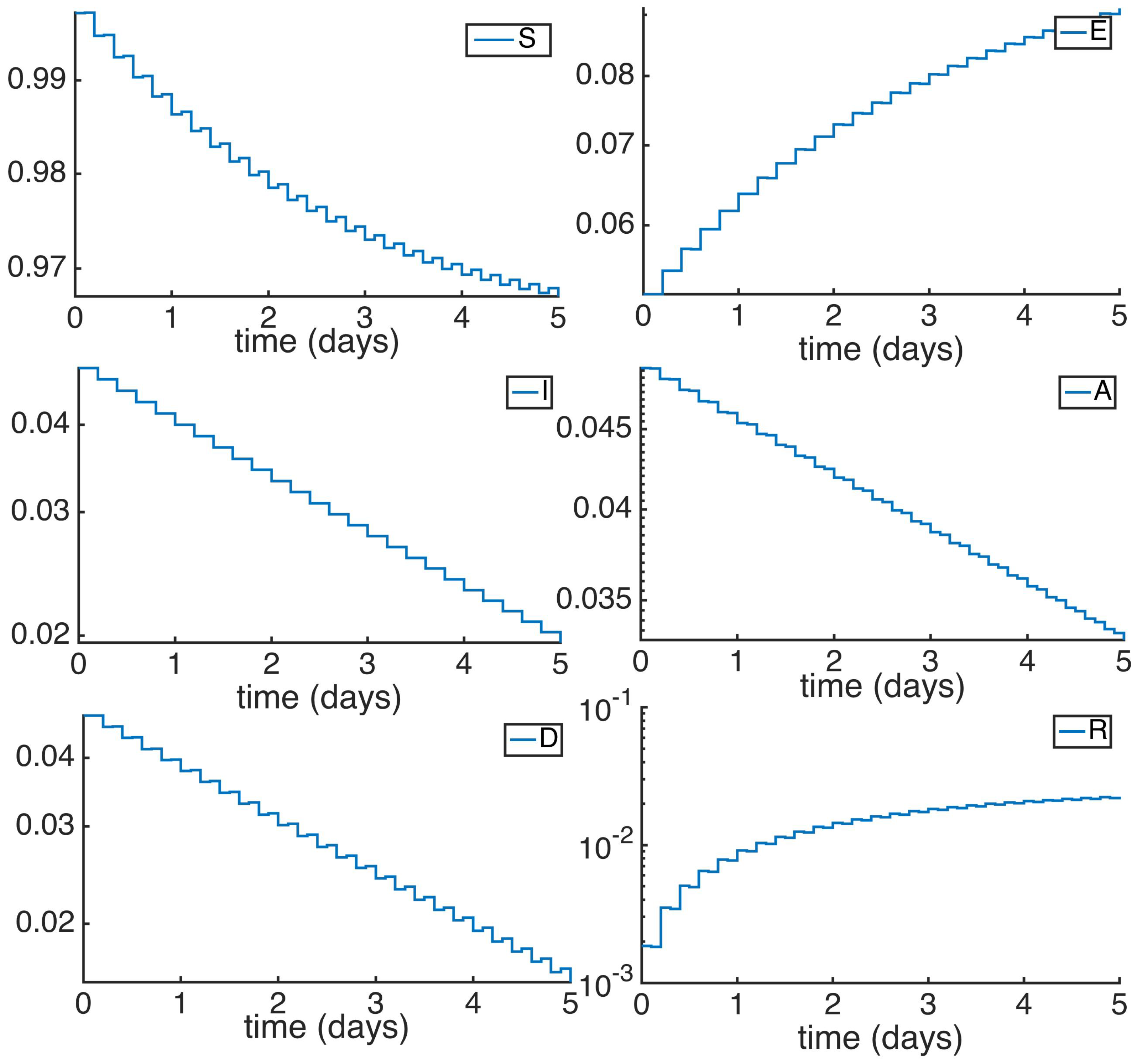
With the susceptible and recovered DFE values as defined in Equation (7). Then, our parameters are set in order to obtain a reproduction number less than unity. The value of the parameters relative to the host population are based in what is expected to be the average rates of growth in a human society, and the ones related to the disease are based on previous models describing Ebola disease [7]. In this way, the mortality and natality rates will be $b_1=b_2=1/(365\times 70){\mathrm{days}}^{-1}$, while the recovery rates from the infection are ${\tau }_0=1/12{\mathrm{days}}^{-1}$, $\mu =1/3{\mathrm{days}}^{-1}$, the parameters of the disease are defined by the infectivity rates $\beta =0.15{\mathrm{days}}^{-1}$, ${\beta }_{\mathrm{A}}=0.02{\mathrm{days}}^{-1}$ and ${\beta }_{\mathrm{D}}=0.15{\mathrm{days}}^{-1}$, the probability of transition $p=0.75$, the mortality of the infected subpopulation $\alpha =0.1{\mathrm{days}}^{-1}$, the transition from infected to recovered $\gamma =1/300{\mathrm{days}}^{-1}$ and the recovered to susceptible rate is defined by $\eta =0.15{\mathrm{days}}^{-1}$. On the other hand, the parameters for the controller methods are defined by the vaccination constants $V=b_1/100{\mathrm{days}}^{-1}$, $K_V=b_2/2{\mathrm{days}}^{-1}$, and the antiviral constant $K_{\xi }=0.01{\mathrm{days}}^{-1}$. Given these conditions, we obtain a reproduction number smaller than unity 1, namely, ${\mathrm{R}}_0=0.81$ and the initial conditions based on the DFE point ${\mathrm{R}}_{\mathrm{DFE}}=1.3\times {10}^{-4}$ and ${\mathrm{S}}_{\mathrm{DFE}}=0.99987$. It can be seen in Figure 1 and Figure 2 the time evolution of the subpopulations given these parameters: The infectious subpopulations decrease exponentially as the susceptible and recovered subpopulations continuously approaches to the values corresponding the DFE point. Note that the simulations are performed to display the trajectory evolution tendencies through time rather than describe real amount of individuals.

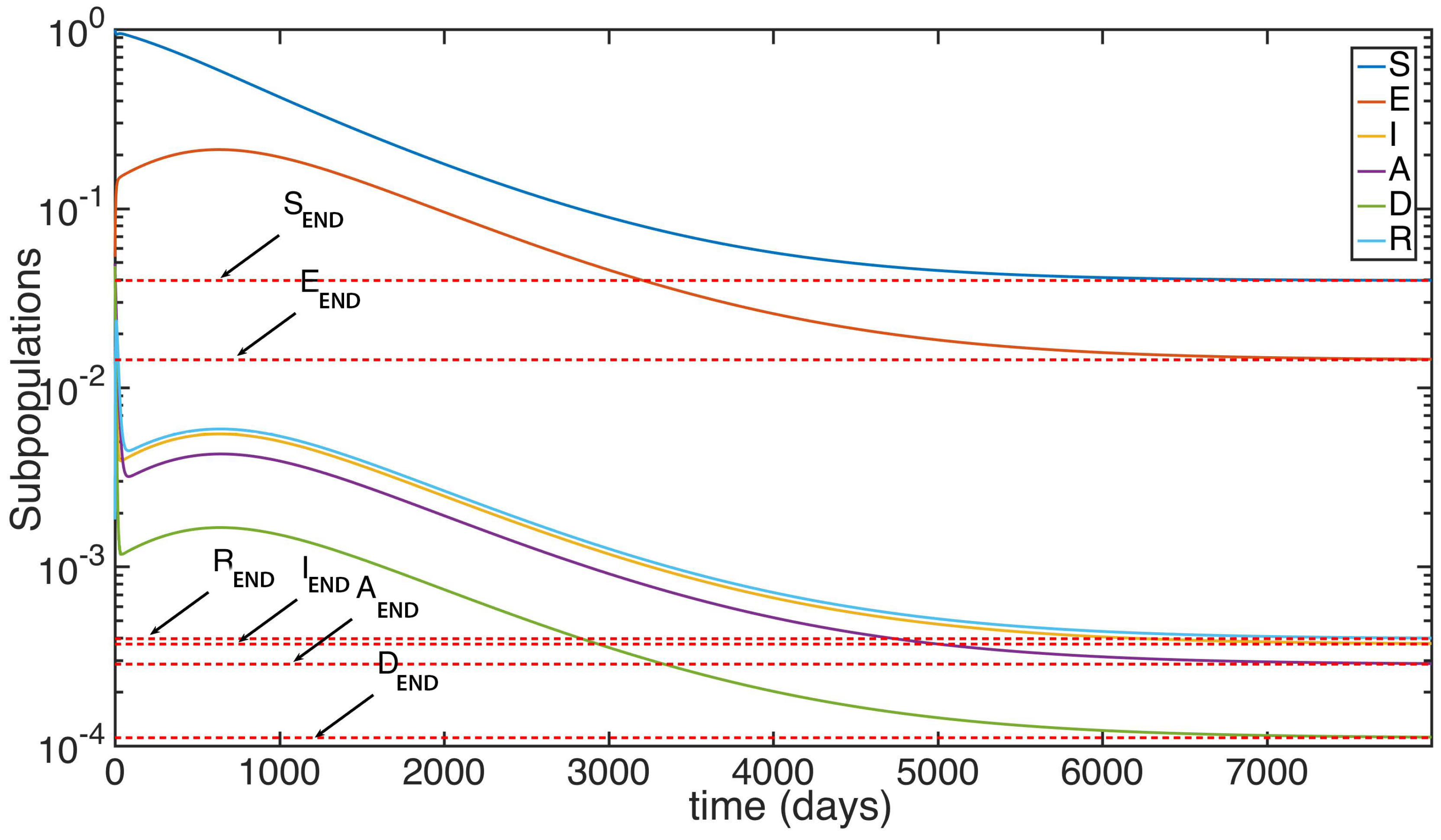
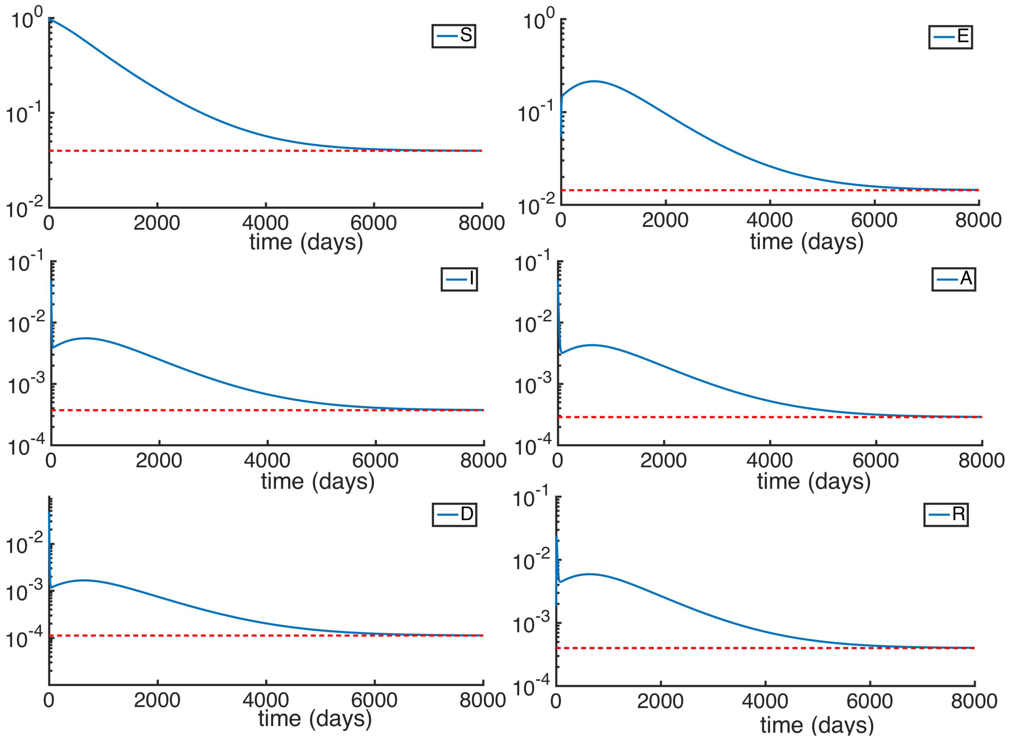
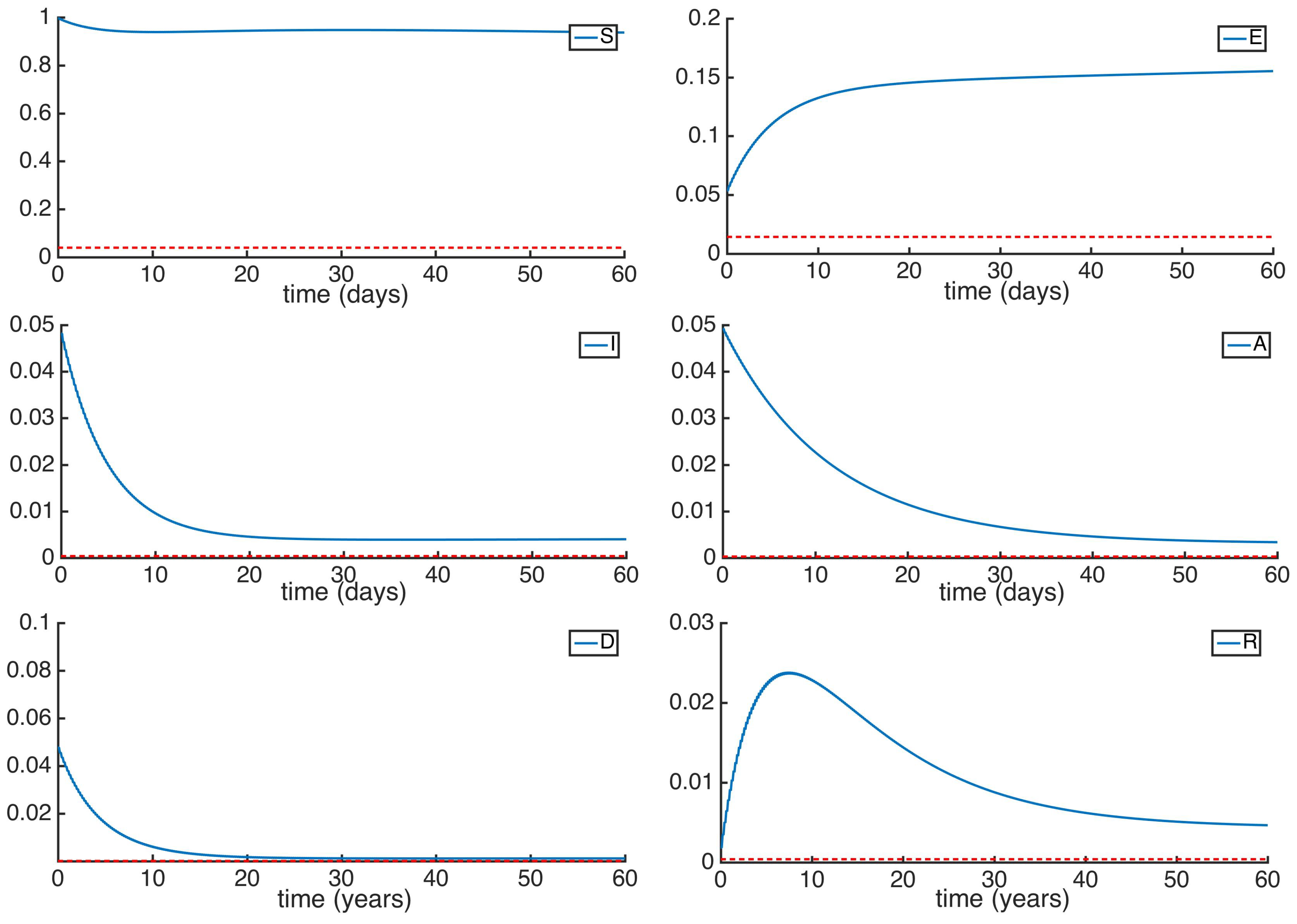
Another simulation is made with the subpopulations starting at the same initial condition that the used in the previous example, but in this time with the reproduction number exceeding unity. The parameters, as in the previous simulation, are based on the average rates of growth in a human society afflicted by an Ebola-type disease. However, the value of the main infectivity rate $\beta$ is changed from $\beta =0.15{\mathrm{days}}^{-1}$ to $\beta =0.30{\mathrm{days}}^{-1}$ so the reproduction number goes from ${\mathrm{R}}_0=0.81$ to ${\mathrm{R}}_0=1.39$. Observe that the change of the infectibity does not change the values of the parameters ${\mathrm{S}}_{\mathrm{DFE}}$ and ${\mathrm{R}}_{\mathrm{DFE}}$, so the initial conditions remain the same. We can see at Figure 3 and Figure 4 the time evolution of the subpopulations reaching the END point. Observe in Figure 4 and Figure 5 that even though given the parameters used in this simulation system takes quite long to stabilize, the subpopulations tend to the endemic values (red dotted).

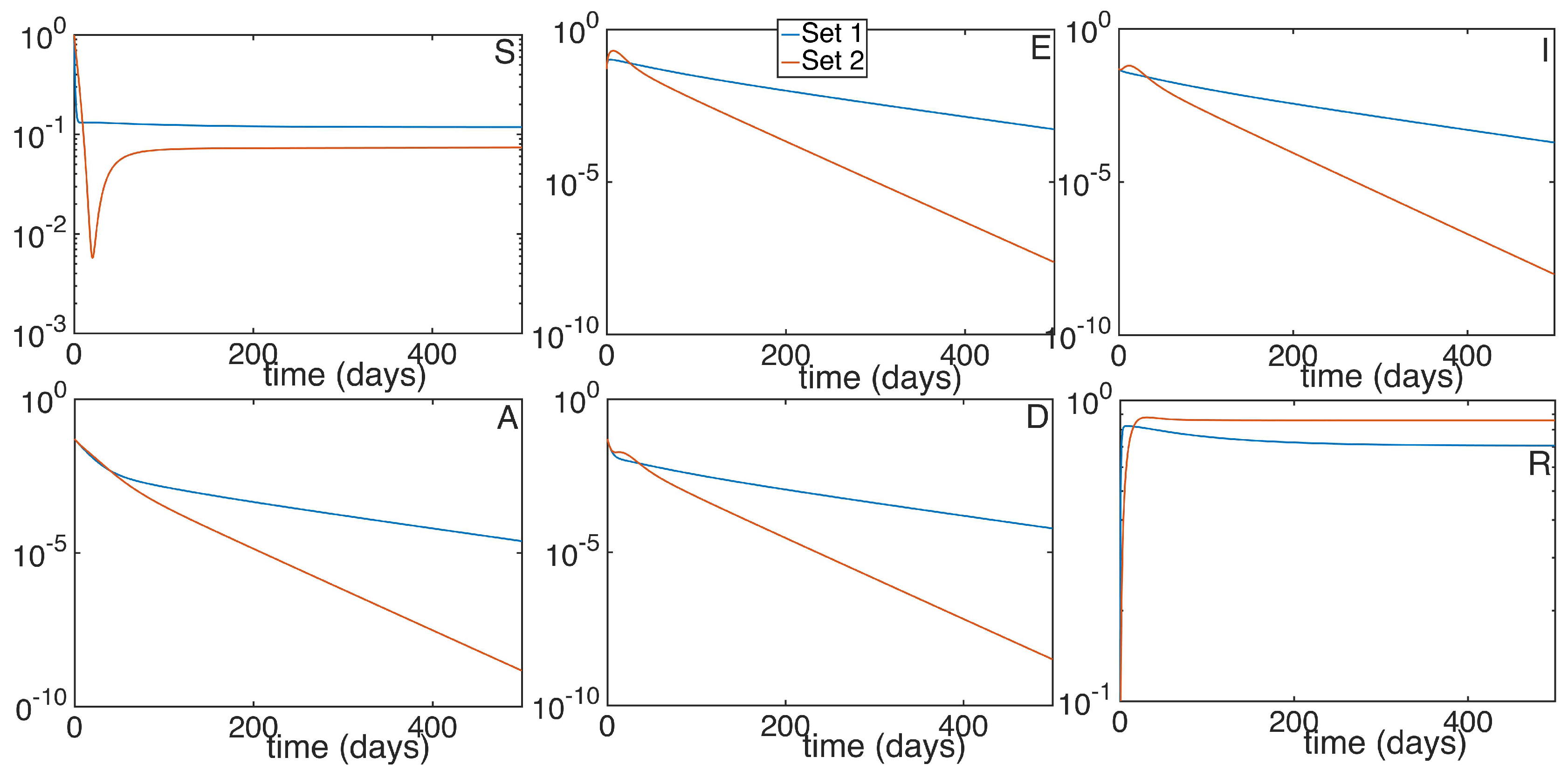
It is worth mentioning that the purpose of running the simulations at such a long time is not with the intention of showing the desired final state of our population, as it would be ridiculous. We want however, to show the general tendency of the dynamic of the subpopulations when the reproduction number exceeds one ( the infectious subpopulations will be relevant for an indefinite time) and when it doesn’t (the infectious subpopulations will decrease exponentially over time). More numerical experimentation has been performed by modifying the control gains while maintaining the reproduction number. The purpose is to study the different velocities at which the subpopulations reach the equilibrium point for a given reproduction number. In this case, the stability properties of the DFE point hold intact depending on the value of ${\mathrm{R}}_0$ being smaller or greater than unity, but the values of the subpopulations corresponding to the equilibrium points of the model and the rate of convergence can be modified. In Figure 6 we can see the dynamics characterized by the parameters of the previous simulations for the infectivity rates $\beta =0.92{\mathrm{days}}^{-1}$, ${\beta }_{\mathrm{A}}=0.2$ and ${\beta }_{\mathrm{D}}=0.5$, and two different sets of vaccination control gains, one corresponding to the constant vaccination strategy and the other one corresponding to the vaccination strategy based on the feedback of the susceptible subpopulation. Both present the same reproduction number and the same values for the subpopulations in the DFE point. However, it is seen that the disease decreases exponentially in both examples, as it is expected when the disease is being eradicated, and that there is a noticeable difference in the presence of the sick individuals. The infectious subpopulations for the set of parameters 2 are larger during the first days, while in the long run they decrease faster than the ones from set 1.

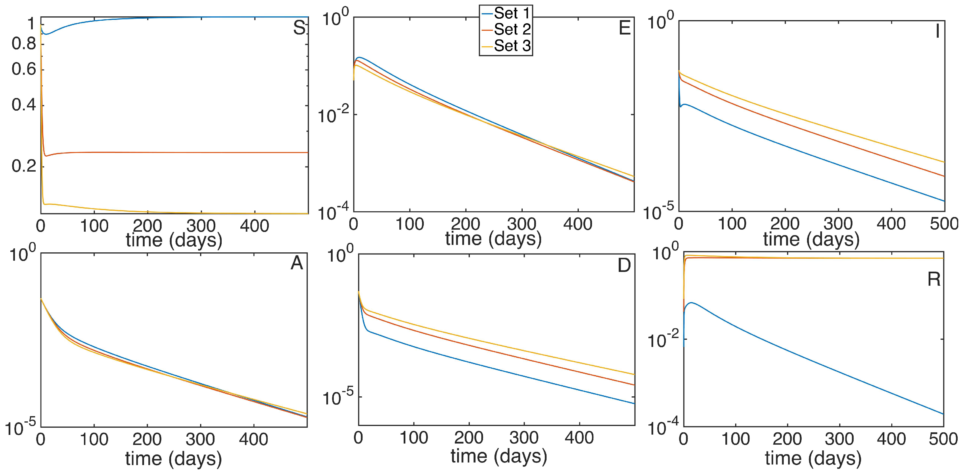
In Figure 7 we show a similar disposition than the previous graphic. With the same parameters as before and $V=0$, we run three different simulations with the same parameters and reproduction number ${\mathrm{R}}_0=0.81$, varying the proportional vaccination control gain $K_V$ and the antiviral treatment control gain $K_{\xi }$.

6. Conclusions

A functional discrete model based on classic models [1,2] describing an Ebola-type disease spreading through a population has been constructed and the control gains applied to synthesize the vaccination and treatment signals are also put into the model successfully. The discrete model has been properly created and the boundaries of the parameters of the simulation are set so that the non-negativity of the system remains as long as the initial conditions are non-negative, as it should be in a model that depicts real populations. Thus, the conditions that guarantee the boundaries of the total population stability of the END and the DFE points have been tested and studied. The simulations presented in this paper also show that the values assigned to the control gain can substantially affect the evolution of the infection. This happens even though the final equilibrium state is the same, which can be used to pick the best strategy when facing humanitarian crisis situations, or when trying to eradicate an endemic disease happening in a region. It can be seen that the increase of the control gains $V,K_v$ and $K_{\xi }$ leads to a computable decrease of the reproduction number (see Equations (31) and (42). It can be seen that the DFE point can be modified with the vaccination control gains, in particular, the susceptible decrease with the constant vaccination V, while the recovered increase with such a control. It can be seen that the disease free susceptible subpopulation decreases as $K_V$ increases, while the recovered increases since the total population remains constant. Also, we have observed the influence of the vaccination control gains in the dynamics even when the reproduction number stays invariant under certain changes of the control gains. This suggests an interesting point when building the control gains of the epidemic models in future works, as it shows that the reproduction number is not the only relevant parameter to be taken into account.

References

- Kermack, W.O.; McKendrick, A.G. A contribution to the mathematical theory of epidemics. Proc. R. Soc. Lond. Ser. A 1927, 115, 700–721. [Google Scholar] [CrossRef]
- Hethcote, H.W. The Mathematics of Infectious Diseases. SIAM Rev. 2000, 42, 599–653. [Google Scholar] [CrossRef] [Green Version]
- Keeling, M.J.; Rohani, P. Modeling Infectious Diseases in Humans and Animals; Princeton University Press: Princeton, NJ, USA; Oxford, UK, 2008. [Google Scholar]
- Hethcote, H.W. Three basic epidemiological models. Appl. Math. Ecol. 1989, 18, 119–144. [Google Scholar]
- Daley, D.; Gani, J. Epidemic Modeling: An Introduction; Cambridge Studies in Mathematical Biology: 15; Cambridge University Press: New York, NY, USA, 2005. [Google Scholar]
- Khan, H.; Mohapatra, R.; Vajravelu, K.; Liao, S.J. The explicit series solution of SIR and SIS epidemic models. Appl. Math. Comput. 2009, 215, 653–669. [Google Scholar] [CrossRef]
- Nistal, R.; De la Sen, M.; Alonso-Quesada, S.; Ibeas, A. A supervised multi-control for monitoring the antiviral treatment strategy for an SEIADR epidemic model. In Proceedings of the 2018 5th International Conference on Control, Decision and Information Technologies (CoDIT), Thessaloniki, Greece, 10–13 April 2018. [Google Scholar]
- Glynn, J.; Bower, H.; Johnson, S.; Houlihan, C.; Montesano, C.; Scott, J.T.; Semple, M.G.; Bangura, M.S.; Kamara, A.J.; Kamara, O.; et al. Asymptotic infection and unrecognised Ebola virus disease in Ebola-affected households in Sierra Leone: A cross-sectional study using new non-invasive assay for antibodies to Ebola virus. Lancet Infect. Dis. 2017, 6, 645–653. [Google Scholar] [CrossRef]
- de Pinho, M.; Maurer, H.; Kornienko, I. Optimal control of a SEIR model with mixed constraints and L1 cost. In Proceedings of the 11th Portuguese Conference on Automatic Control Lecture Notes in Electrical Engineering, Porto, Portugal, 21–23 July 2014. [Google Scholar]
- Leroy, E.; Baize, S.; Volchkov, V.; Fisher-Hoch, S.P.; Georges-Courbot, M.C.; Lansoud-Soukate, J.; Capron, M.; Debre, P.; Georges, A.J.; McCormick, J.B. Human asymptomatic Ebola infection and strong inflammatory response. Lancet 2000, 355, 2210–2215. [Google Scholar] [CrossRef]
- Bellan, S.; Pulliam, J.; Dushoff, J.; Meyers, L. Ebola control: Effect of asymptomatic infection and acquired immunity. Lancet 2014, 384, 1499–1500. [Google Scholar] [CrossRef]
- Santermans, E.; Robesyn, E.; Sudre, T.G.B.; Faes, C.; Quinten, C.; Van Bortel, W.; Haber, T.; Kovac, T.; Reeth, F.V.; Testa, M.; et al. Spatiotemporal evolution of Ebola disease at sub-national level during the 2014 West Africa epidemic: Model scrutiny and data meagerness. PLoS ONE 2016, 11, e0147172. [Google Scholar] [CrossRef]
- Al-Darabsah, I.; Yuan, Y. A time-delayed epidemic model for Ebola disease transmission. Appl. Math. Comput. 2016, 290, 307–325. [Google Scholar] [CrossRef]
- De la Sen, M.; Agarwal, R.P.; Ibeas, A.; Alonso-Quesada, S. On the existence of equilibrium points, boundedness, oscillating behaviour and positivity of a SVEIRS epidemic model under constant and impulsive vaccination. Adv. Differ. Equ. 2011, 2011, 748608. [Google Scholar] [CrossRef]
- De la Sen, M.; Alonso-Quesada, S. Vaccination strategies based on feedback control techniques for a SEIR-epidemic model. Appl. Math. Comput. 2011, 218, 3888–3904. [Google Scholar] [CrossRef]
- Wei, Z.; Le, M. Existence and Convergence of the Positive Solutions of a Discrete Epidemic Model. Discret. Dyn. Nat. Soc. 2015, 2015, 434537. [Google Scholar] [CrossRef]
- Wang, L.; Liu, Z.; Zhang, X. Global dynamics of an SVEIR epidemic model with distributed delay and nonlinear incidence. Appl. Math. Comput. 2016, 2016, 47–65. [Google Scholar] [CrossRef]
- Wang, X. An SIRS Epidemic Model with Vital Dynamics and a Ratio-Dependent Saturation Incidence Rate. Discret. Dyn. Nat. Soc. 2015, 2015, 720682. [Google Scholar] [CrossRef]
- Fengying, W.; Chen, F. Stochastic permanence of an SIQS epidemic model with saturated incidence and independent random perturbations. Phys. A Stat. Mech. Its Appl. 2016, 453, 99–107. [Google Scholar]
- De la Sen, M.; Alonso-Quesada, S.; Ibeas, A. On the stability of an SEIR epidemic model with distributed time-delay and a general class of feedback vaccination rules. Appl. Math. Comput. 2015, 270, 953–976. [Google Scholar] [CrossRef]
- Shaikhet, L. Stability of equilibrium states for a stochastically perturbed exponential type system of differential equations. J. Comput. Appl. Math. 2015, 290, 92–103. [Google Scholar] [CrossRef]
- Shaikhet, L.; Korobeinikov, A. Stability of a stochastic model for HIV-1 dynamics within a host. Appl. Anal. 2016, 95, 1228–1238. [Google Scholar] [CrossRef]
- De la Sen, M.; Agarwal, R.P.; Ibeas, A.; Alonso-Quesada, S. On a generalized time-varying SEIR epidemic model with mixed point and distributed time-varying delays and combined regular and impulsive vaccination. Adv. Diff. Equ. 2010, 2010, 281612. [Google Scholar] [CrossRef]
- Tripathi, J.; Abbas, S. Global dynamics of autonomous and nonautonomous SI epidemic models with nonlinear incidence rate and feedback controls. Nonlinear Dyn. 2016, 86, 337–351. [Google Scholar] [CrossRef]
- Buonomo, B.; Lacitignola, D.; de Leon, C.V. Qualitative analysis and optimal control of an epidemic model with vaccination and treatment. Math. Comput. Simul. 2014, 100, 88–102. [Google Scholar] [CrossRef]
- Ling, L.; Jiang, G.; Long, T. The dynamics of an SIS epidemic model with fixed-time birth pulses and state feedback pulse treatments. Appl. Math. Model. 2015, 39, 5579–5591. [Google Scholar] [CrossRef]
- He, Y.; Gao, S.; Xie, D. An SIR epidemic model with time-varying pulse control schemes and saturated infectious force. Appl. Math. Model. 2013, 37, 8131–8140. [Google Scholar] [CrossRef]
- Sharma, S.; Samanta, G. Stability analysis and optimal control of an epidemic model with vaccination. Int. J. Biomath. 2015, 8, 1550030. [Google Scholar] [CrossRef]
- Samanta, G. A delayed hand-foot-mouth disease model with pulse vaccination strategy. Comput. Appl. Math. 2015, 34, 1131–1152. [Google Scholar] [CrossRef]
- De la Sen, M.; Ibeas, A. On the global asymptotic stability of switched linear time-varying systems with constant point delays. Discret. Dyn. Nat. Soc. 2008, 2008, 231710. [Google Scholar] [CrossRef]
- Bilbao-Guillerna, A.; De la Sen, M.; Ibeas, A.; Alonso-Quesada, S. Robustly stable multiestimation scheme for adaptive control and identification. Discret. Dyn. Nat. Soc. 2005, 2015, 31–67. [Google Scholar] [CrossRef]
- Bilbao-Guillerna, A.; De la Sen, M.; Alonso-Quesada, S. Multimodel discrete control with online updating of the fractional order hold gains. Cybern. Syst. 2007, 38, 249–274. [Google Scholar] [CrossRef]
- Herrera, J.; Ibeas, A.; Alcantara, S.; De la Sen, M. Multimodel-based techniques for the identification and adaptive control of delayed multi-input multi-output systems. IET Control Theory Appl. 2011, 5, 188–202. [Google Scholar] [CrossRef]
- Jang, S. On a discrete west Nile epidemic model. Comput. Appl. Math. 2007, 6, 397–414. [Google Scholar] [CrossRef]
- Zhao, J.; Wang, L.; Han, Z. Stability analysis of two new SIRS models with two viruses. Int. J. Comput. Math. 2018, 95, 2026–2035. [Google Scholar] [CrossRef]
- Degue, K.; Ny, J.L. An interval observer for discrete-time SEIR epidemic model. In Proceedings of the 2018 American Control Conference (ACC), Milwaukee, WI, USA, 27–29 June 2018; pp. 5934–5939. [Google Scholar]
- Chang, C.; Jing, Y.; Zhu, B. Modeling and control for a descriptor epidemic system with nonlinear incidence rate. In Proceedings of the 2018 Chinese Control Conference (CCDC), Shenyang, China, 27–29 June 2018; pp. 2183–2188. [Google Scholar]
- Abdelaziz, M.; Ismail, A.I.; Abdullah, F.; Mohd, M.H. Bifurcations and chaos in a discrete SI epidemic model with fractional order. Adv. Diff. Equ. 2018, 44, 1–19. [Google Scholar] [CrossRef]
- Chiranjeevi, T.; Biswas, B. Discrete-time fractional optimal control. Mathematics 2017, 5, 25. [Google Scholar] [CrossRef]
- De la Sen, M. Preserving positive realness through discretization. Positivity 2002, 6, 31–45. [Google Scholar] [CrossRef]
Figure 1.
Time evolution of the different subpopulations for a .
Figure 2.
A detailed display of the reaction of the different subpopulations during the first days after the introduction of the disease given a .
Figure 3.
Time evolution of the different subpopulations given a .
Figure 4.
A better display of the different subpopulations for a .
Figure 5.
A close look at the beginning of the dynamic simulation of the different subpopulations for a .
Figure 6.
Time evolution of the different subpopulations given a and two different sets of control vaccination gains. Set 1 shares common parameters with set 2 except for and , while set 2 presents and .
Figure 7.
Time evolution of the different subpopulations given a and three different sets of control vaccination gains. Set 1 shares common parameters with set 2 and 3, except for and , while set 2 presents and and set 3 and .
© 2018 by the authors. Licensee MDPI, Basel, Switzerland. This article is an open access article distributed under the terms and conditions of the Creative Commons Attribution (CC BY) license (http://creativecommons.org/licenses/by/4.0/).
Share and Cite
MDPI and ACS Style
Nistal, R.; De la Sen, M.; Alonso-Quesada, S.; Ibeas, A. On a New Discrete SEIADR Model with Mixed Controls: Study of Its Properties. Mathematics 2019, 7, 18. https://doi.org/10.3390/math7010018
AMA Style
Nistal R, De la Sen M, Alonso-Quesada S, Ibeas A. On a New Discrete SEIADR Model with Mixed Controls: Study of Its Properties. Mathematics. 2019; 7(1):18. https://doi.org/10.3390/math7010018
Chicago/Turabian StyleNistal, Raul, Manuel De la Sen, Santiago Alonso-Quesada, and Asier Ibeas. 2019. "On a New Discrete SEIADR Model with Mixed Controls: Study of Its Properties" Mathematics 7, no. 1: 18. https://doi.org/10.3390/math7010018
Note that from the first issue of 2016, this journal uses article numbers instead of page numbers. See further details here.