Abstract
Moth search (MS) algorithm, originally proposed to solve continuous optimization problems, is a novel bio-inspired metaheuristic algorithm. At present, there seems to be little concern about using MS to solve discrete optimization problems. One of the most common and efficient ways to discretize MS is to use a transfer function, which is in charge of mapping a continuous search space to a discrete search space. In this paper, twelve transfer functions divided into three families, S-shaped (named S1, S2, S3, and S4), V-shaped (named V1, V2, V3, and V4), and other shapes (named O1, O2, O3, and O4), are combined with MS, and then twelve discrete versions MS algorithms are proposed for solving set-union knapsack problem (SUKP). Three groups of fifteen SUKP instances are employed to evaluate the importance of these transfer functions. The results show that O4 is the best transfer function when combined with MS to solve SUKP. Meanwhile, the importance of the transfer function in terms of improving the quality of solutions and convergence rate is demonstrated as well.
1. Introduction
The knapsack problem (KP) [] is still considered as one of the most challenging and interesting classical combinatorial optimization problems, because it is non-deterministic polynomial hard problem and has many important applications in reality. As an extension of the standard 0–1 knapsack problem (0–1 KP) [], the set-union knapsack problem (SUKP) [] is a novel KP model recently introduced in [,]. The SUKP finds many practical applications such as financial decision making [], data stream compression [], flexible manufacturing machine [], and public key prototype [].
The classical 0–1 KP is one of the simplest KP model in which each item has a unique value and weight. However, SUKP is constructed of a set of items S = {U1, U2, U3, …, Um} and a set of elements U = {u1, u2, u3, …, un}. Each item is associated with a subset of elements. In SUKP, each item has a nonnegative profit and each element has a nonnegative weight. The goal is to maximize the total profit of a subset of items such that the total weight of the corresponding element does not exceed the maximum capacity of knapsack C. Hence, SUKP is more complicated and more difficult to handle than the standard 0–1 KP. Thus far, only a few researchers have studied this issue despite its practical importance and NP-hard character. For example, Goldschmidt et al. applied the dynamic programming (DP) algorithm for SUKP []. However, when the exact algorithm is used, no satisfactory approximate solution is usually obtained in polynomial time. Afterwards, Ashwin [] proposed an approximation algorithm A-SUKP for SUKP. Obviously, A-SUKP also has to face the inevitable problem, that is, how to compromise between achieving a high-quality solution and exponential runtime. Recently, He et al. [] presented a binary artificial bee colony algorithm (BABC) to solve SUKP and comparative studies were conducted among BABC, A-SUKP, and binary differential evolution (DE) []. The results verified that BABC outperformed A-SUKP method. Ozsoydan et al. [] proposed a swarm intelligence-based algorithm for the SUKP and designed an effective mutation procedure. Although this method does not require transfer functions, it lacks generality. Therefore, it is urgent to find an efficient metaheuristic algorithm to address SUKP whether from the perspective of academic research or practical application.
As a relatively novel nature-inspired metaheuristic algorithm, moth search (MS) algorithm was recently developed for continuous optimization by Wang []. Computational experiments have shown that MS is not only effective but also efficient when addressing unconstrained continuous optimization problems, compared with five state-of-the-art metaheuristic algorithms. Because of its relative novelty, extensive research on MS is relatively scarce, especially discrete version MS algorithm. Feng et al. presented a binary moth search algorithm (BMS) for discounted {0–1} knapsack problem (DKP) [].
As we all know, the metaheuristic algorithm is usually discretized in two ways: direct discretization and indirect discretization. Direct discretization is usually achieved by modifying the evolutionary operator of the original algorithm to solve a particular discrete problem. This method depends on the algorithm used and the problem solved. Obviously, the disadvantages of direct discretization are lack of versatility and complicated operation. The latter is discretized by establishing a mapping relationship between continuous space and discrete space. Concretely speaking, indirect discretization is usually achieved by an appropriate transfer function to convert real-valued variables into discrete variables. Many discrete versions of swarm intelligence algorithms using transfer functions have been proposed to solve various optimization problems. Discrete binary particle swarm optimization [], discrete firefly algorithm [], and binary harmony search algorithm [] are among the most typical algorithms. Through analyzing the literature, many kinds of transfer functions can be used, such as sigmoid function [], tanh function [], etc. However, most existing metaheuristics only consider one transfer function. Little research concentrates on the importance of transfer functions in solving discrete problems. In addition, a few studies [,] investigate the efficiency of multiple transfer functions.
In this paper, twelve principal transfer functions are used and then twelve new discrete MS algorithms are proposed to solve SUKP. These functions include four S-shaped transfer functions [,], named S1, S2, S3, and S4, respectively; four V-shaped transfer functions [,], named V1, V2, V3, and V4, respectively; and four other shapes transfer functions (Angle modulation method [,], Nearest integer method [,], Normalization method [], and Rectified linear unit method []), named O1, O2, O3, and O4, respectively. Therefore, combining twelve transfer functions with MS algorithm, twelve discrete MS algorithms are naturally proposed, named as MSS1, MSS2, MSS3, MSS4, MSV1, MSV2, MSV3, MSV4, MSO1, MSO2, MSO3, and MSO4, respectively.
The remainder of the paper is organized as follows. In Section 2, we briefly introduce the SUKP problem and MS algorithm. The families of transfer functions and repair optimization mechanism are presented in Section 3. In Section 4, the twelve discrete MS algorithms are compared to shed light on how the transfer functions affect the performance of the algorithm. After that, the best algorithm (MSO4) is compared with five state-of-the-art methods on fifteen SUKP instances. Finally, we draw conclusions and suggest some directions for future research.
2. Background
To describe discrete MS algorithm for the SUKP, we first explain the mathematical model of SUKP and then introduce the MS algorithm.
2.1. Set-Union Knapsack Problem
The set-union knapsack problem (SUKP) [,] is a variant of the classical 0–1 knapsack problem (0–1 KP). More formally, the SUKP can be defined as follows: given a set of elements U = {u1, u2, u3, …, un} and a set of items S = {U1, U2, U3, …, Um}, such that S is the cover of U, and (i = 1, 2, 3, …, m) and each item Ui has a value pi > 0. Each element uj (j = 1, 2, 3, …, n) has a weight wj > 0. Suppose that set A consists of some items packed into the knapsack with capacity C, namely . Then, the profit of A is defined as and the weight of A is defined as . The objective of the SUKP is to find a subset A that maximizes the total value P(A) on condition that the total weight W(A) C. Then, the mathematical model of SUKP can be formulated as follows:
where pi (i = 1, 2, 3, …, m), wj (j = 1, 2, 3, …, n), and C are all positive integers.
Recently, an integer programming model is proposed by He et al. [] to solve SUKP easily by using metaheuristic algorithm; the new mathematical model of SUKP can be defined as follows:
Obviously, all the 0–1 vectors Y = [y1, y2, y3, …, ym] are the potential solutions of SUKP. A solution satisfying the constraint of Equation (4) is a feasible solution; otherwise, it is an infeasible solution. AY = {Ui|yi Y, yi = 1, 1 ≤ i ≤ m} S. Then, yi = 1 if and only if Ui AY.
2.2. Moth Search Algorithm
The MS algorithm [] is a novel metaheuristic algorithm that was inspired by the phototaxis and Lévy flights of the moths in nature, which are the two most representative characteristics of moths. The MS is akin to other population-based swarm intelligence algorithms. However, MS differs from most the population-based metaheuristic algorithms, such as genetic algorithm (GA) [,] and particle swarm optimization algorithm (PSO) [,], which consist of only one population, as, in MS, the whole population is divided into two subpopulations according to the fitness, namely subpopulation1 and subpopulation2.
The MS starts its evolutionary process by first randomly generating n moth individuals. Each moth individual represents a candidate solution to the corresponding problem with a specific fitness function. In MS, two operators are considered including Lévy flights operator and straight flight operator. Correspondingly, an individual update in subpopulation1 and subpopulation2 is generated by performing Lévy flights operator and straight flight operator, respectively.
- Lévy flights: For each individual i in subpopulation1, it will fly around the best one in the form of Lévy flights. The resulting new solution is calculated based on Equations (5)–(7).where xit and xit+1 denote the position of moth i at generation t and t + 1, respectively. denotes the scale factor related to specific problem. Smax is the max walk step and it takes the value 1.0 in this paper. L(s) represents the step drawn from Lévy flights and is the gamma function. In this paper, = 1.5 and s can be regarded as the position of moth individual in the solution space then is the power of s.
- Straight flights: for each individual i in subpopulation2, it will fly towards that source of light in line. The resulting new solution is formulated as Equation (8).where and represent scale factor and acceleration factor, respectively. xtbest is the best individual at generation t. Rand is a function generating a random number uniformly distributed in (0, 1).
3. Discrete MS Optimization Method for SUKP
In this section, we describe the newly proposed discrete MS for SUKP. The main purpose of extending MS algorithm to solve the novel SUKP is to investigate the significant role of the transfer functions in terms of improving the quality of solutions and convergence rate. The basic MS algorithm was initially proposed for continuous optimization problems, while SUKP belongs to a discrete optimization problem with constraints. Therefore, the SUKP problem must contain three key elements, namely, discretization method, solution representation, and constraint handling. The three key elements are described in detail subsequently.
3.1. Transfer Functions
Transfer function is a major contributor of the discrete MS algorithm; therefore, it deserves special attention and research. In this section, 12 transfer functions are introduced. According to the shape of transfer function curve, we divide the twelve transfer functions into three groups: S-shaped transfer functions [], V-shaped transfer functions [], and other-shaped (O-shaped) transfer functions [,]. As described above, each group consists of four functions, which are named as Si, Vi, and Oi (i = 1, 2, 3, 4), respectively. These transfer functions are presented in Table 1 and Figure 1.

Table 1.
Twelve transfer functions.
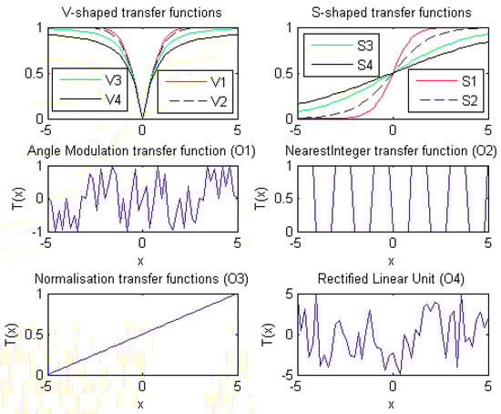
Figure 1.
Twelve transfer functions.
As stated in the literature [,], the transfer functions define the probability that the element of position vector of each moth individual changes from 0 to 1, and vice versa. Therefore, an appropriate transfer function should ensure that a real-valued vector in a continuous search space is mapped to the value 1 in a binary search space with greater probability. Suppose applying the transfer function T(x) will return a function value y (y = 1 or y = 0) through a mapping method. The probability of a transfer function with a value of 1 (PR) is displayed in Figure 2. Three groups of items, namely, 100 items, 300 items, and 500 items, were selected to count the PR value:
where N represents the number of items. The value of longitudinal axis in Figure 2 is the average of PR among 100 independent runs.
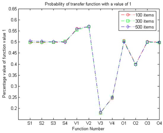
Figure 2.
Probability of transfer function with a value of 1.
As shown in Figure 2, the four S-shaped transfer functions have similar PR values, which are close to 0.5. However, the PR values of the four V-shaped transfer functions differ considerably. V2 has the best PR value while the PR value of V3 is less than 0.2. It seems that V3 combining with MS should show poor performance. Similarly, V4 also demonstrates unsatisfactory performance, with a PR value of less than 0.25. Of the four other shapes of transfer functions, O1, O3, and O4 obtain a similar PR value, that is, close to 0.5. The PR value of O2 is slightly smaller than that of O1, O3, and O4. In sum, according to the preliminary analysis of PR values, it seems that V3, V4, and O2 are not suitable for combining with MS to solve binary optimization problems.
3.2. Solution Representation
The basic MS is a real-valued algorithm and each moth individual is represented as a real-valued vector. Two main operators are defined in continuous space. However, SUKP is a discrete optimization problem with constraints and the solution is a binary vector. In this paper, the most general and simplest method, mapping the real-valued vectors into binary ones by transfer functions, is opted. Concretely speaking, a real-valued vector X = [x1, x2, …, xm] [−a, a]m still evolves in continuous space. Here, m is the number of items and a is a positive real value, and a = 5.0 in this paper. Then, transfer function T(x) is used to map X into a binary vector Y = [y1, y2, …, ym] {0, 1}m. According to the feature of these transfer functions, three mapping methods are as follows.
The first mapping method: Choose a transfer function from S1–S4, V1–V4, and O3.
where rand( ) is a random number in (0, 1). In Figure 1, it can be observed that S-shaped transfer functions, V-shaped transfer functions, and O3 will return a random real number between 0 and 1. Therefore, the comparison of rand( ) to T(xi) equals 1 or 0. Then, the mapping procedure is shown as Table 2.
Table 2.
The first mapping procedure according to S2 transfer function.
The second mapping method: Choose the transfer function O2.
The third mapping method: Choose either O1 or O4 as the transfer function.
Then, the quality of any feasible solution Y is evaluated by the objective function f of the SUKP. Given a potential solution Y = [y1, y2, …, ym], the objective function value f(Y) is defined by
3.3. Repair Mechanism and Greedy Optimization
Clearly, SUKP is a kind of important combinatorial optimization problem with constraints. Due to the existence of constraints, the feasible search space of decision variables becomes irregular, which will increase the difficulty of finding the optimal solution. Among the many constraint processing techniques, repairing the infeasible solution is a common method to solve the combinatorial optimization problem. Michalewicz [] introduced an evolutionary system based on repair technology. Obviously, repairing technique is dependent on specific problems and different repairing method must be designed for different problems. Consequently, He et al. [] designed a repairing and optimization algorithm (named S-GROA) for SUKP, which can not only repair infeasible solutions but also further optimize feasible solutions. On the basis of S-GROA [], a quadratic greedy repair and optimization strategy (QGROS) is proposed by Liu et al. []. In this paper, QGROS is adopted. The preprocessing phase of QGROS can be summarized as follows:
- (1)
- Compute the frequency dj of the element j (j = 1, 2, 3, …, n) in the subsets U1, U2, U3, …, Um.
- (2)
- Calculate the unit weight Ri of the item i (i = 1, 2, 3, …, m).
- (3)
- Record the profit density of each item in S according to PDi.
- (4)
- Sort all the items in a non-ascending order based on PDi (i = 1, 2, 3, …, m) and then the index value recorded in an array H[1…m].
- (5)
- Define a term for any binary vector Y = [y1, y2, …, ym] {0, 1}m.
The pseudocode of QGROS [] is outlined in Algorithm 1.
| Algorithm 1. QGROS algorithm for SUKP. |
| Begin Step 1: Input: the candidate solution , H[1…m]. Step 2: Initialization. The m-dimensional binary vector Z = [0, 0, …, 0]. Step 3: Greedy repair stage For i = 1 to m do If . End if End for Y Z. Step 4: Quadratic greedy stage Do not consider the elements that have been packed into the knapsack, recalculate dj (j = 1, 2, 3, …, n), Ri (i = 1, 2, 3, … m), and H[1…m] Step 5: Optimization sate For i = 1 to m do If . End if End for Step 6: Output: End. |
In Algorithm 1, we can observe that QGROS consists of three stages. The first stage is determining whether the constraints are met for the items in the potential solution that are ready to be packed into the knapsack. At this stage, items in the potential solution that are intended to be packed into knapsack but violate constraints will be removed. Therefore, all solutions are feasible after this stage. The second stage is recalculating the frequency of each element, the unit weight of each item, and the array H[1…m]. The third stage is optimizing the remaining items by loading appropriate items into the knapsack with the aim of maximizing the use of the remaining capacity. At this stage, items in the feasible solution that are not intended to be loaded in the knapsack but satisfy the constraints will be loaded. Hence, after this stage, all solutions remain feasible and the quality of solutions is improved.
3.4. The Main Scheme of Discrete MS for SUKP
Having discussed all the components of the discrete MS algorithms in detail, the complete procedure is outlined in Algorithm 2.
3.5. Computational Complexity of the Discrete MS Algorithm
Computational complexity is the main criterion for evaluating the running time of an algorithm, which can be calculated according to its structure and implementation. In Algorithm 2, it can be seen that the computing time in each iteration is mainly dependent on the number of moths, problem dimension, and sorting of items as well as moth individual in each iteration. In addition, the computational complexity is mainly determined by Steps 1–4. In Step 1, since the Quicksort algorithm is used, the average and the worst computational costs are O(mlogm) and O(m2), respectively. In Step 2, the initialization of N moth individuals costs time O(N × m) = O(m2). In Step 3, the fitness calculation of N moth individuals costs time O(N). In Step 4, Lévy flight operator has time complexity O(N/2 × m) = O(m2), straight flight operator has time complexity O(N/2 × m) = O(m2), QGROS has time complexity O(m × n), and sorting the population with Quicksort has average time complexity and worst time complexity of O(NlogN) and O(N2), respectively. Consequently, the overall computational complexity is O(mlogm) + O(m2) + O(N) + O(m2) + O(m2) + O(m × n) + O(NlogN) = O(m2), where m is the number of items and N is the number of moths.
| Algorithm 2. The main procedure of discrete MS algorithm for SUKP. |
| Begin Step 1: Sorting. Sort all items in S in non-increasing order according to PDi (), and the indexes of items are recorded in array H [0…m]. Step 2: Initialization. Set the maximum iteration number MaxGen and iteration counter G = 1; = 1.5; the acceleration factor = 0.618. Generate N moth individuals randomly {X1, X2, …, XN}, Xi [−a, a]m. Divide the whole population into two subpopulations with equal size: subpopulation1 and subpopulation2, according to their fitness. Calculate the corresponding binary vector Yi = T(Xi) by using transfer functions (i = 1, 2, …, N). Perform repair and optimization with QGROS. Step 3: Fitness calculation. Calculate the initial fitness of each individual, f(Yi), 1 ≤ i ≤ N. Step 4: While G < MaxGen do Update subpopulation 1 by using Lévy flight operator. Update subpopulation 2 by using fly straightly operator. Calculate the corresponding binary vector Yi = T(Xi) by using transfer functions (i = 1, 2, …, N). Perform repair and optimization with QGROS. Evaluate the fitness of the population and record the <Xgbest, Ygbest>. G = G + 1. Recombine the two newly-generated subpopulations. Sort the population by fitness. Divide the whole population into subpopulation 1 and subpopulation 2. Step 5: End while Step 6: Output: the best results. End. |
4. Results and Discussion
In this section, we present experimental studies on the proposed discrete MS algorithms for solving SUKP.
Test instance: Three groups of thirty SUKP instances were recently presented by He et al. []. What needs to be specified is that the set of items S = {U1, U2, U3, …, Um} is represented as a 0–1 matrix M = (rij), with m rows and n columns. For each element rij in M (i = 1, 2, …, m; j = 1, 2, …, n), rij = 1 if and only if uj = Ui. Therefore, each instance contains four factors: (1) m denotes the number of items; (2) n denotes the number of elements; (3) density of element 1 in the matrix M {0.1, 0.15}; and (4) the ratio of C to the sum of all elements {0.75, 0.85}. According to the relationship between m and n, three types of instances are generated. The first group: 10 SUKP instances with m > n, m {100, 200, 300, 400, 500} and n {85, 185, 285, 385, 485}, named as F01–F10, respectively. The second group: 10 SUKP instances with m = n, m {100, 200, 300, 400, 500} and n {100, 200, 300, 400, 500}, named as S01–S10, respectively. The third group: 10 SUKP instances with m < n, m {85, 185, 285, 385, 485} and n {100, 200, 300, 400, 500}, named as T01–T10, respectively. We selected five instances in each group with = 0.1 and = 0.75. The instances can be downloaded at http://sncet.com/ThreekindsofSUKPinstances(EAs).rar. Three categories with different relationships between m and n (m > n, m = n, and m < n) of 15 SUKP instances were selected for testing. The parameters and the best solution value (Best*) [] are shown in Table 3.
Table 3.
The parameters and the best solution value provided in [] for 15 SUKP instances.
Experimental environment: For fair comparisons, all proposed algorithms in this paper were coded in C++ and in the Microsoft Visual Studio 2015 environment. All the experiments were run on a PC with Intel (R) Core (TM) i7-7500 CPU (2.90 GHz and 8.00 GB RAM).
On the stopping condition, we followed the original paper [] and set the iteration number MaxGen equal to max {m, n} for all SUKP instances. Here, m denotes the number of items and n is the number of elements in each SUKP instance. In addition, the population size of all the algorithms was set to N = 20. For each SUKP instance, we carried out 100 independent replications.
The parameters for the proposed discrete MS algorithms were set as follows: the max step Smax = 1.0, acceleration factor = 0.618, and the index = 1.5.
4.1. The Performance of Discrete MS Algorithm with Different Transfer Functions
Computational results are summarized in Table 4, which records the results for SUKP instances with m > n, m = n, and m < n, respectively. For each instance, we give several criteria to evaluate the comprehensive performance of the twelve discrete MS algorithms. “Best” and “Mean” refer to the best value and the average value for each instance obtained by each algorithm among 100 independent runs. The best solution provided in [] are given in parentheses in the first column.
Table 4.
The best values and average values of twelve discrete MS algorithms on 15 SUKP instances.
In Table 4, it can be easily observed that MSO4 outperforms the eleven other discrete MS algorithms and demonstrates the best comprehensive performance when solving all fifteen SUKP instances. In addition, MSS2 and MSO3 show comparable performance.
To evaluate the performance of each algorithm, the relative percentage deviation (RPD) was defined to represent the similarity between the best value obtained by each algorithm and the best solution 5. The RPD of each SUKP instance is calculated as follows.
where is the best solution provided in []. Clearly, if the value of RPD is less than 0, the algorithm updates the best solution of the SUKP test instance in []. The statistical results are shown in Table 5.
Table 5.
The effect of twelve transfer functions on the performance of discrete MS algorithm (RPD values).
In Table 5, it can be seen that, in all twelve discrete MS algorithms, MSS2, MSS3, MSV4, MSO1, MSO3, and MSO4 all update the best solutions []. However, MSS3 and MSV4 update only one SUKP instance, T05. MSO1 updates the instances F07, F09, S07, and T05. Moreover, MSO4 still keeps the best performance because its total average RPD is only −1.28. The total average RPD of MSO3 is −0.14, which implies that MSO3 is slightly worse than MSO4 but outperforms the ten other discrete MS algorithms. Obviously, MSS2 is the third best of the twelve discrete MS algorithms. Indeed, it can also be seen that MSO4 updates and obtains the best solutions [] ten and two times (out of 15), i.e., 66.67% and 13.33% of the whole instance set, respectively. MSO3 updates and fails to find the best solutions 5 nine and six times (out of 15), i.e., 60.00% and 40.00% of the whole instance set, respectively. MSS2 updates and obtains the best solutions 5 eight (53.33%) and one times (6.60%), respectively.
To further evaluate the comprehensive performance of twelve discrete MS algorithms in solving fifteen SUKP instances, the average ranking based on the best values are displayed in Table 6 and Figure 3, respectively. In Table 6 and Figure 3, the average ranking value of MSO4 is 1.60 and it still ranks first. In addition, MSO3 and MSS2 are the second and the third best algorithms, respectively, which is very consistent with the previous analysis. The ranking of twelve discrete MS algorithms based on the best values are as follows:
Table 6.
Ranks of twelve discrete MS algorithms based on the best values.
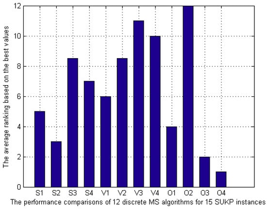
Figure 3.
Comparison of the average rank of 12 discrete MS algorithms for 15 SUKP instances.
By looking closely at Figure 2 and Figure 3, it is not difficult to see that V3, V4, and O2 exhibit the worst performance, which is consistent in the two figures. Similar to the previous analysis in Figure 2, O1, O3, and O4 show satisfactory performance among 12 transfer functions. Thus, it can be inferred that PR value can be used as a criterion for selecting transfer functions.
To analyze the experimental results for statistical purposes, we selected three representative instances (F09, S09, and T09) and provided boxplots in Figure 4, Figure 5 and Figure 6. In Figure 4, the boxplot of MSS2 has greater value and less height than those of other eleven algorithms. In Figure 5 and Figure 6, MSO3 exhibits a similar phenomenon as MSS2 in Figure 4. Additionally, the performance of MSO2 is the worst. In Figure 4, Figure 5 and Figure 6, we can also observe that MSO3 performs slightly better than MSO4 in solving large-scale instances.
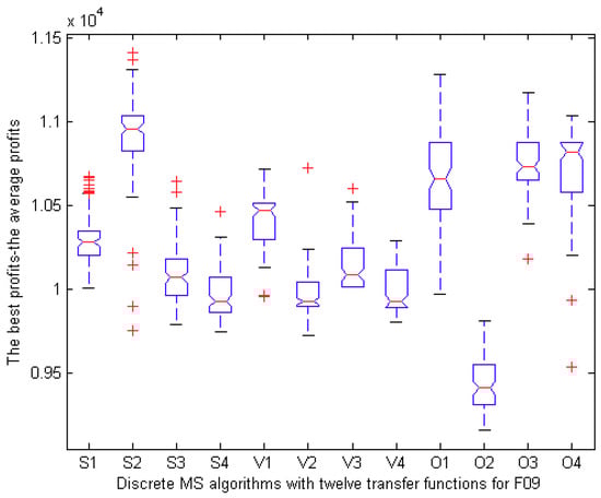
Figure 4.
Boxplot of the best values on F09 in 100 runs.
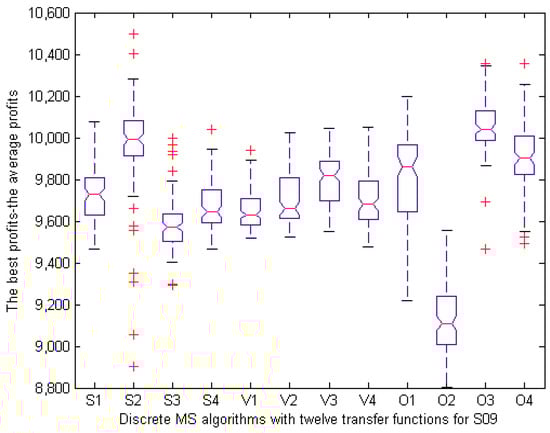
Figure 5.
Boxplot of the best values on S09 in 100 runs.
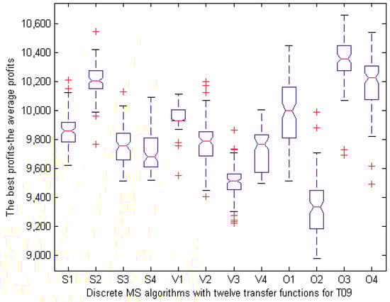
Figure 6.
Boxplot of the best values on T09 in 100 runs.
Moreover, optimization process of each algorithm in solving F09, S09, and T09 instances is given in Figure 7, Figure 8 and Figure 9, respectively. In these three figures, all the function values are the average best values achieved from 100 runs. In Figure 7, the initial value of MSS2 is greater than that of other algorithms and then it quickly converges to the global optimum. For MSO3, the same scene appears in Figure 8 and Figure 9. Overall, MSS2 and MSO3 have stronger optimization ability and faster convergence speed than the other discrete MS algorithms.
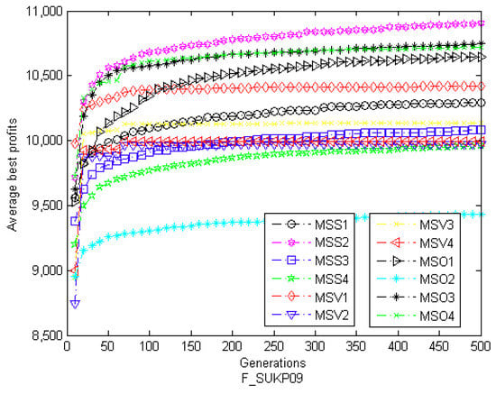
Figure 7.
The convergence graph of twelve discrete MS algorithms on F09.
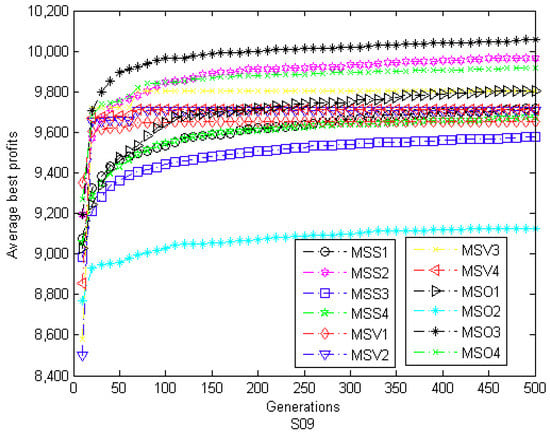
Figure 8.
The convergence graph of twelve discrete MS algorithms on S09.
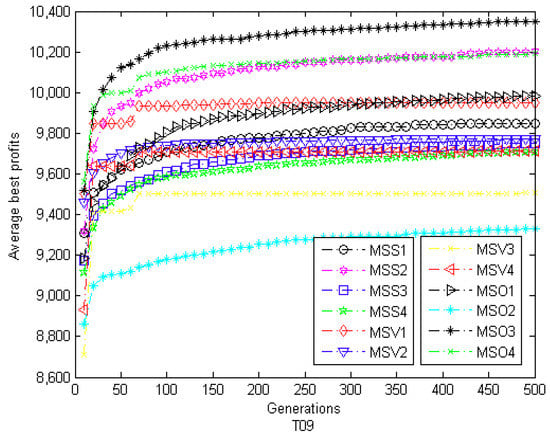
Figure 9.
The convergence graph of twelve discrete MS algorithms on T09.
Through the above experimental analysis, the following conclusions can be drawn: (1) For S-shaped transfer functions, the combination of S2 and MS (MSS2) is the most effective. (2) As far as V-shaped transfer functions are concerned, the combination of V1 and MS (MSV1) shows the best performance. (3) In the case of other shapes transfer functions, the more effective algorithms are MSO4, MSO3, and MSO1. (4) By comparing the family of S-shaped transfer functions and V-shaped transfer functions, the family of S-shaped transfer functions with MS is suitable for solving SUKP problem. (5) MSO4 has advantages over other algorithms in terms of the quality of solutions. (6) As far as the stability and convergence rate are concerned, MSO3 and MSS2 perform better than other algorithms.
Overall, it is evident that MSO4 has the best results (considering RPD values and average ranking values) on fifteen SUKP instances. Therefore, it appears that the proposed other-shapes family of transfer functions, particularly the O4 function, has many advantages combined with other algorithms to solve binary optimization problems. Additionally, the O3 function and S2 function are also suitable functions that can be considered for selection. In brief, these results demonstrate that the transfer function plays a very important role in solving SUKP using discrete MS algorithm. Thus, by carefully selecting the appropriate transfer function, the performance of discrete MS algorithm can be improved obviously.
4.2. Estimation of the Solution Space
SUKP is a binary coded problem and the solution space can be represented as a graph G = (V, E), in which vertex set V = S, where S is the set of solutions for a SUKP instance, S = {0, 1}n and edge set , where dmin is the minimum distance between two points in the search space. Especially, hamming distance is used to describe the similarity between individuals. Obviously, the minimum distance is 0 when all bits have the same value and the maximum distance is n, where n is the dimension of SUKP instance.
Here, MSO4 is specially selected to analyze the solution space for F01, S01, and T01 SUKP instance. The distribution of fitness at generation 0 and generation 100 is presented in Figure 10, Figure 11 and Figure 12. The distance between each individual and the best individual is given in Figure 13, Figure 14 and Figure 15. In Figure 10, Figure 11 and Figure 12, we can see that, at generation 0, the fitness values are more dispersed and worse than that at generation 100. In Figure 13, it can be observed that the hamming distance varies from 0 to 35 at generation 0 while the range is 0 to 12 at generation 100. Moreover, the hamming distance can be divided into eight levels at generation 100, which demonstrates that all individuals tend to some superior individuals. However, this phenomenon is not evident in S01 and T01.
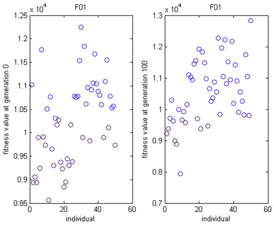
Figure 10.
The distribution graph of fitness on MSO4 for F01.
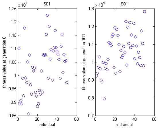
Figure 11.
The distribution graph of fitness on MSO4 for S01.
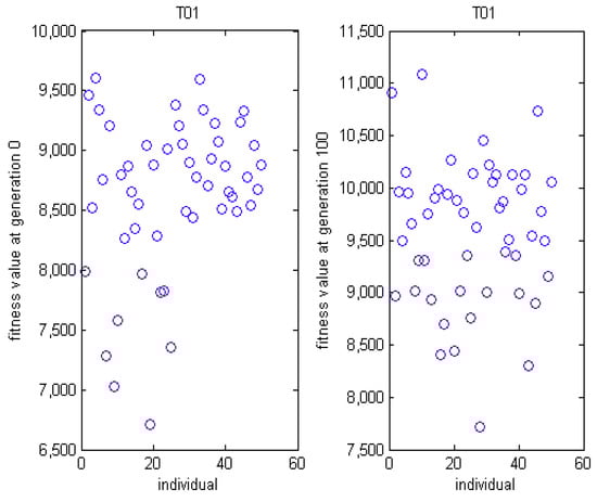
Figure 12.
The distribution graph of fitness on MSO4 for T01.
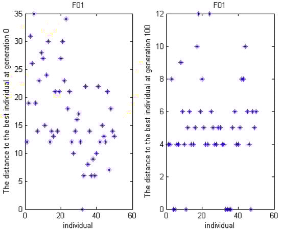
Figure 13.
The distance to the best individual for F01.
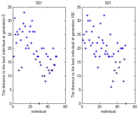
Figure 14.
The distance to the best individual for S01.
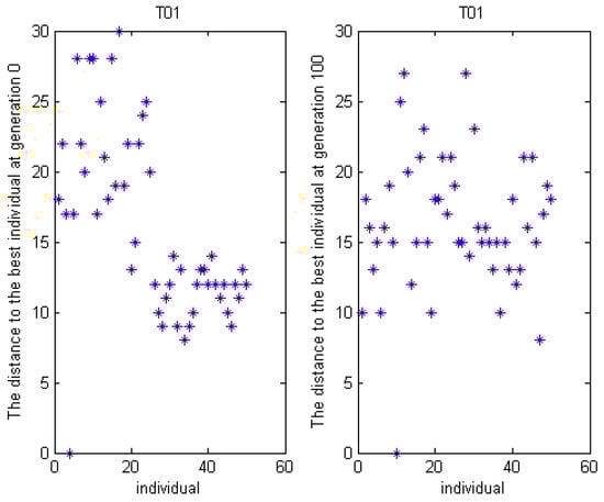
Figure 15.
The distance to the best individual for T01.
To intuitively understand the similarity of the solutions, the spatial structure of the solutions at generation 100 is illustrated in Figure 16, Figure 17 and Figure 18. In Figure 16, the first node (denoting the first individual) has the maximum degree which also shows more individuals have approached the better individual. However, the value of degree is not much different in Figure 17 and Figure 18. This result is consistent with the previous analysis.
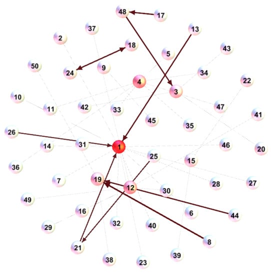
Figure 16.
The spatial structure graph for F01 at generation 100.
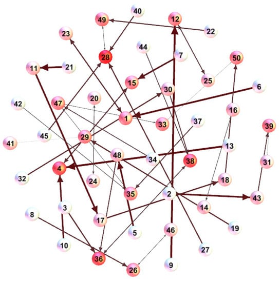
Figure 17.
The spatial structure graph for S01 at generation 100.
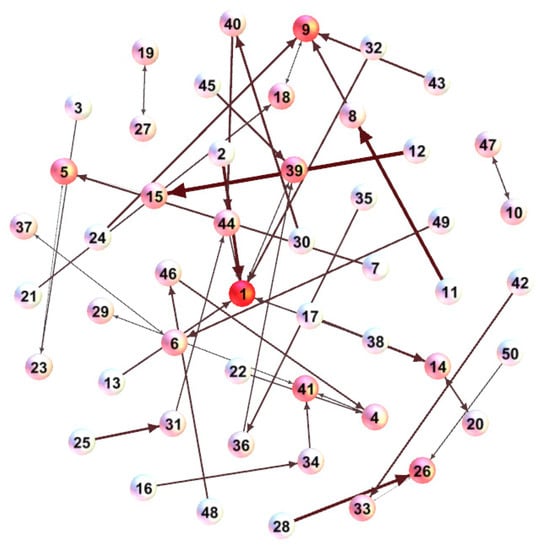
Figure 18.
The spatial structure graph for T01 at generation 100.
4.3. Discrete MS Algorithm vs. Other Optimization Algorithms
To further verify the performance of discrete MS algorithm, we chose MSO4 algorithm to compare with five other optimization algorithms. These comparison algorithms include PSO [], DE [], global harmony search (GHS) [], firefly algorithm (FA) [], and monarch butterfly optimization (MBO) [,]. In DE, the DE/rand/1/bin scheme was adopted. PSO, FA, and MBO are classical or novel swarm intelligence algorithms that simulate the social behavior of birds, firefly, and monarch butterfly, respectively. DE is derived from evolutionary theory in nature and has been proved to be one of the most promising stochastic real-value optimization algorithms. GHS is an efficient variant of HS, which imitates the music improvisation process. It is also noteworthy that all five comparison algorithms adopt the discretization method introduced in this paper and combine with O4, respectively. The parameter setting for each algorithm are shown in Table 7.
Table 7.
The parameter settings of six algorithms on SUKP.
The best results and average results obtained by six methods over 100 independent runs as well the average time cost of each computation (unit: second, represented as “time”) are summarized in Table 8. The frequency (TBest and TMean) and average ranking (RBest and RMean) of each algorithm with the best performance based on the best values and average values are also recorded in Table 8. The average time cost of each computation for solving fifteen SUKP instances is illustrated in Figure 19. In Table 8, on best, MSO4 outperforms other methods on eight of fifteen instances (F01, F03, F05, F07, S01, S03, S05, and T03). MBO is the second most effective. In terms of average ranking, there is little difference between the performance of MSO4 and MBO. In terms of the average time cost, it can be observed in Figure 19 that DE has the slowest computing speed. However, GHS has surprisingly fast solving speed. In addition, MSO4 is second among the six algorithms. Overall, the computing speed of PSO, FA, MBO and MSO4 shows little difference.
Table 8.
Computational results and comparisons on the Best and Mean on 15 SUKP instances.
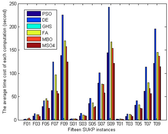
Figure 19.
The average time cost of each computation for solving fifteen SUKP instances.
To investigate the difference between the results obtained by MSO4 and those by the comparison algorithm from the perspective of statistics, Wilcoxon’s rank sum tests with the 5% significance level were performed. The results of rank sum tests are recorded in Table 9. In Table 9, “1” and “−1” indicate that MSO4 is superior or inferior to the corresponding comparison algorithm, respectively, while “0” shows that there is no statistical difference at 5% significance level between the two comparison algorithms. The statistical result is shown in Table 9.
Table 9.
Results of rank sum tests for MSO4 with the comparison algorithms.
In Table 8, MSO4 outperforms PSO and DE on all fifteen instances. In addition, MSO4 performs better than GHS and FA on most of the instances except for S05 and F01, respectively. Meanwhile, MSO4 is superior to MBO on eleven instances except for F07, F09, S01, and S05. Statistically, there is no difference between the performance of MSO4 and that of MBO for these four instances.
5. Conclusions
In this paper, twelve different transfer functions-based discrete MS algorithms are proposed for solving SUKP. These transfer functions can be divided into three families, S-shaped, V-shaped, and other-shaped transfer functions. To investigate the performance of twelve discrete MS algorithms, three groups of fifteen SUKP instances were employed and the experimental results were compared and analyzed comprehensively. From the experimental results, we found that MSO4 has the best performance. Furthermore, the relative percentage deviation (RPD) was calculated to evaluate the similarity between the best value obtained by each algorithm and the best solution provided in []. The results show that six algorithms update the best solutions [] for 11 SUKP instances. The results also indicate that four other shapes transfer functions, especially the O4 function combined with MS, have merits for solving discrete optimization problems.
The comparison results on the fifteen SUKP instances among MSO4 and five state-of-the-art algorithms show that MSO4 performs competitively.
There are several possible directions for further study. First, we will investigate some new transfer functions on other algorithms such as krill herd algorithm (KH) [,,,,], fruit fly optimization algorithm (FOA) [], earthworm optimization algorithm (EWA) [], and cuckoo search (CS) [,]. Second, we will study other techniques to discrete continuous optimization algorithms such as k-means framework []. Third, we will apply these twelve transfer functions-based discrete MS algorithms to other related and more complicated binary optimization problems including multidimensional knapsack problem (MKP) [] and flow shop scheduling problem (FSSP) []. Finally, we will incorporate other strategies, namely, information feedback [] and chaos theory [], into MS to improve the performance of the algorithm.
Author Contributions
Writing and methodology, Y.F.; supervision, H.A.; review and editing, X.G.
Funding
This research was funded by National Natural Science Foundation of China, grant number 61806069, Key Research and Development Projects of Hebei Province, grant number 17210905.
Conflicts of Interest
The authors declare no conflict of interest.
References
- Cormen, T.H.; Leiserson, C.E.; Rivest, R.L.; Stein, C. Introduction to Algorithms; MIT Press: Cambridge, MA, USA, 2009. [Google Scholar]
- Du, D.Z.; Ko, K.I. Theory of Computational Complexity; John Wiley Sons: Hoboken, NJ, USA, 2011. [Google Scholar]
- Goldschmidt, O.; Nehme, D.; Yu, G. Note: On the set-union knapsack problem. Naval Res. Logist. (NRL) 1994, 41, 833–842. [Google Scholar] [CrossRef]
- Arulselvan, A. A note on the set union knapsack problem. Discret. Appl. Math. 2014, 169, 214–218. [Google Scholar] [CrossRef]
- He, Y.; Xie, H.; Wong, T.L.; Wang, X. A novel binary artificial bee colony algorithm for the set-union knapsack problem. Future Gener. Comput. Syst. 2017, 78, 77–86. [Google Scholar] [CrossRef]
- Yang, X.; Vernitski, A.; Carrea, L. An approximate dynamic programming approach for improving accuracy of lossy data compression by Bloom filters. Eur. J. Oper. Res. 2016, 252, 985–994. [Google Scholar] [CrossRef]
- Schneier, B. Applied Cryptography: Protocols, Algorithms, and Source Code in C; John Wiley Sons: Hoboken, NJ, USA, 2007. [Google Scholar]
- Engelbrecht, A.P.; Pampara, G. Binary differential evolution strategies. In Proceedings of the IEEE Congress on Evolutionary Computation, Singapore, 25–28 September 2007; pp. 1942–1947. [Google Scholar]
- Ozsoydan, F.B.; Baykasoglu, A. A swarm intelligence-based algorithm for the set-union knapsack problem. Future Gener. Comput. Syst. 2018, 93, 560–569. [Google Scholar] [CrossRef]
- Wang, G.G. Moth search algorithm: A bio-inspired metaheuristic algorithm for global optimization problems. Memetic Comput. 2016. [Google Scholar] [CrossRef]
- Feng, Y.; Wang, G.G. Binary moth search algorithm for discounted 0-1 knapsack problem. IEEE Access 2018, 6, 10708–10719. [Google Scholar] [CrossRef]
- Kennedy, J.; Eberhart, R.C. A discrete binary version of the particle swarm algorithm. In Proceedings of the 1997 IEEE International Conference on Systems, Man, and Cybernetics—Computational Cybernetics and Simulation, Orlando, FL, USA, 12–15 October 1997; Volume 5, pp. 4104–4108. [Google Scholar]
- Karthikeyan, S.; Asokan, P.; Nickolas, S.; Page, T. A hybrid discrete firefly algorithm for solving multi-objective flexible job shop scheduling problems. Int. J. Bio-Inspired Comput. 2015, 7, 386–401. [Google Scholar] [CrossRef]
- Kong, X.; Gao, L.; Ouyang, H.; Li, S. A simplified binary harmony search algorithm for large scale 0-1 knapsack problems. Expert Syst. Appl. 2015, 42, 5337–5355. [Google Scholar] [CrossRef]
- Rashedi, E.; Nezamabadi-Pour, H.; Saryazdi, S. BGSA: Binary gravitational search algorithm. Nat. Comput. 2010, 9, 727–745. [Google Scholar] [CrossRef]
- Saremi, S.; Mirjalili, S.; Lewis, A. How important is a transfer function in discrete heuristic algorithms. Neural Comput. Appl. 2015, 26, 625–640. [Google Scholar] [CrossRef]
- Mirjalili, S.; Lewis, A. S-shaped versus V-shaped transfer functions for binary particle swarm optimization. Swarm Evol. Comput. 2013, 9, 1–14. [Google Scholar] [CrossRef]
- Pampara, G.; Franken, N.; Engelbrecht, A.P. Combining particle swarm optimisation with angle modulation to solve binary problems. In Proceedings of the 2005 IEEE Congress on Evolutionary Computation, Edinburgh, UK, 2–5 September 2005; Volume 1, pp. 89–96. [Google Scholar]
- Leonard, B.J.; Engelbrecht, A.P.; Cleghorn, C.W. Critical considerations on angle modulated particle swarm optimisers. Swarm Intell. 2015, 9, 291–314. [Google Scholar] [CrossRef]
- Costa, M.F.P.; Rocha, A.M.A.C.; Francisco, R.B.; Fernandes, E.M.G.P. Heuristic-based firefly algorithm for bound constrained nonlinear binary optimization. Adv. Oper. Res. 2014, 2014, 215182. [Google Scholar] [CrossRef]
- Burnwal, S.; Deb, S. Scheduling optimization of flexible manufacturing system using cuckoo search-based approach. Int. J. Adv. Manuf. Technol. 2013, 64, 951–959. [Google Scholar] [CrossRef]
- Pampará, G.; Engelbrecht, A.P. Binary artificial bee colony optimization. In Proceedings of the 2011 IEEE Symposium on Swarm Intelligence (SIS), Paris, France, 11–15 April 2011; pp. 1–8. [Google Scholar]
- Zhu, H.; He, Y.; Wang, X.; Tsang, E.C.C. Discrete differential evolutions for the discounted {0-1} knapsack problem. Int. J. Bio-Inspired Comput. 2017, 10, 219–238. [Google Scholar] [CrossRef]
- Changdar, C.; Mahapatra, G.S.; Pal, R.K. An improved genetic algorithm based approach to solve constrained knapsack problem in fuzzy environment. Expert Syst. Appl. 2015, 42, 2276–2286. [Google Scholar] [CrossRef]
- Lim, T.Y.; Al-Betar, M.A.; Khader, A.T. Taming the 0/1 knapsack problem with monogamous pairs genetic algorithm. Expert Syst. Appl. 2016, 54, 241–250. [Google Scholar] [CrossRef]
- Cao, L.; Xu, L.; Goodman, E.D. A neighbor-based learning particle swarm optimizer with short-term and long-term memory for dynamic optimization problems. Inf. Sci. 2018, 453, 463–485. [Google Scholar] [CrossRef]
- Chih, M. Three pseudo-utility ratio-inspired particle swarm optimization with local search for multidimensional knapsack problem. Swarm Evol. Comput. 2017, 39. [Google Scholar] [CrossRef]
- Michalewicz, Z.; Nazhiyath, G. Genocop III: A co-evolutionary algorithm for numerical optimization problems with nonlinear constraints. In Proceedings of the 1995 IEEE International Conference on Evolutionary Computation, Perth, Western Austrilia, 29 November–1 December 1995; Volume 2, pp. 647–651. [Google Scholar]
- Liu, X.J.; He, Y.C.; Wu, C.C. Quadratic greedy mutated crow search algorithm for solving set-union knapsack problem. In Microelectro. Comput.; 2018; Volume 35, pp. 13–19. [Google Scholar]
- Omran, M.G.H.; Mahdavi, M. Global-best harmony search. Appl. Math. Comput. 2008, 198, 643–656. [Google Scholar] [CrossRef]
- Yang, X.S. Firefly Algorithm, Lévy Flights and Global Optimization. In Research and Development in Intelligent Systems XXVI; Springer: London, UK, 2010; pp. 209–218. [Google Scholar]
- Wang, G.-G.; Deb, S.; Cui, Z. Monarch butterfly optimization. Neural Comput. Appl. 2015, 1–20. [Google Scholar] [CrossRef]
- Feng, Y.; Wang, G.G.; Li, W.; Li, N. Multi-strategy monarch butterfly optimization algorithm for discounted {0-1} knapsack problem. Neural Comput. Appl. 2017, 1–18. [Google Scholar] [CrossRef]
- Wang, G.-G.; Gandomi, A.H.; Alavi, A.H. An effective krill herd algorithm with migration operator in biogeography-based optimization. Appl. Math. Model. 2014, 38, 2454–2462. [Google Scholar] [CrossRef]
- Wang, G.-G.; Gandomi, A.H.; Alavi, A.H. Stud krill herd algorithm. Neurocomputing 2014, 128, 363–370. [Google Scholar] [CrossRef]
- Wang, G.; Guo, L.; Wang, H.; Duan, H.; Liu, L.; Li, J. Incorporating mutation scheme into krill herd algorithm for global numerical optimization. Neural Comput. Appl. 2014, 24, 853–871. [Google Scholar] [CrossRef]
- Wang, H.; Yi, J.-H. An improved optimization method based on krill herd and artificial bee colony with information exchange. Memetic Comput. 2017. [Google Scholar] [CrossRef]
- Wang, G.-G.; Deb, S.; Gandomi, A.H.; Alavi, A.H. Opposition-based krill herd algorithm with Cauchy mutation and position clamping. Neurocomputing 2016, 177, 147–157. [Google Scholar] [CrossRef]
- Wang, L.; Zheng, X.L.; Wang, S.Y. A novel binary fruit fly optimization algorithm for solving the multidimensional knapsack problem. Knowl.-Based Syst. 2013, 48, 17–23. [Google Scholar] [CrossRef]
- Wang, G.-G.; Deb, S.; Coelho, L.D.S. Earthworm optimization algorithm: A bio-inspired metaheuristic algorithm for global optimization problems. Int. J. Bio-Inspired Comput. 2015. [Google Scholar] [CrossRef]
- Cui, Z.; Sun, B.; Wang, G.-G.; Xue, Y.; Chen, J. A novel oriented cuckoo search algorithm to improve DV-Hop performance for cyber-physical systems. J. Parallel. Distr. Comput. 2017, 103, 42–52. [Google Scholar] [CrossRef]
- Wang, G.-G.; Gandomi, A.H.; Zhao, X.; Chu, H.E. Hybridizing harmony search algorithm with cuckoo search for global numerical optimization. Soft Comput. 2016, 20, 273–285. [Google Scholar] [CrossRef]
- García, J.; Crawford, B.; Soto, R.; Castro, C.; Paredes, F. A k-means binarization framework applied to multidimensional knapsack problem. Appl. Intell. 2018, 48, 357–380. [Google Scholar] [CrossRef]
- Deng, J.; Wang, L. A competitive memetic algorithm for multi-objective distributed permutation flow shop scheduling problem. Swarm Evolut. Comput. 2016, 32, 107–112. [Google Scholar] [CrossRef]
- Wang, G.-G.; Tan, Y. Improving metaheuristic algorithms with information feedback models. IEEE Trans. Cybern. 2017. [Google Scholar] [CrossRef] [PubMed]
- Wang, G.-G.; Guo, L.; Gandomi, A.H.; Hao, G.-S.; Wang, H. Chaotic krill herd algorithm. Inf. Sci. 2014, 274, 17–34. [Google Scholar] [CrossRef]
© 2018 by the authors. Licensee MDPI, Basel, Switzerland. This article is an open access article distributed under the terms and conditions of the Creative Commons Attribution (CC BY) license (http://creativecommons.org/licenses/by/4.0/).