Two-Level Finite Element Approximation for Oseen Viscoelastic Fluid Flow

Abstract

In this paper, a two-level finite element method for Oseen viscoelastic fluid flow obeying an Oldroyd-B type constitutive law is presented. With the newly proposed algorithm, solving a large system of the constitutive equations will not be much more complex than the solution of one linearized equation. The viscoelastic fluid flow constitutive equation consists of nonlinear terms, which are linearized by taking a known velocity $\mathbf{b}\left(x\right)$, and transforms into the Oseen viscoelastic fluid flow model. Since Oseen viscoelastic fluid flow is already linear, we use a two-level method with a new technique. The two-level approach is consistent and efficient to study the coupled system which contains nonlinear terms. In the first step, the solution on the coarse grid is derived, and the result is used to determine the solution on the fine mesh in the second step. The decoupling algorithm takes two steps to solve a linear system on the fine mesh. The stability of the algorithm is derived for the temporal discretization and obtains the desired error bound. Two numerical experiments are executed to show the accuracy of the theoretical analysis. The approximations of the stress tensor, velocity vector, and pressure field are $P1$-discontinuous, $P2$-continuous and $P1$-continuous finite elements respectively.

1. Introduction

In nature, most fluids are non-Newtonian, and many researchers have investigated the behaviour of non-Newtonian fluid extensively. Non-Newtonian fluid has numerous applications in different sectors such as in the natural substances, in food processing, and biological fluid. Some familiar examples of the natural substances are magma, lava, gums and so on. In the food processing area: butter, cheese, jam, ketchup, soap, yogurt, and in the biological fluid flow sector: blood, saliva, mucus, synovial fluids, are all examples of non-Newtonian fluid. Viscoelastic fluid is one of the essential non-Newtonian fluid which satisfies both the viscous property of the fluid and elastic estate of solid. Over the last few decades, the developments of viscoelastic fluid research have achieved significant progress, but the rheological properties of the viscoelastic fluid is not similar as Newtonian fluid. To describe the viscoelastic behaviour of the liquid, it was a significant challenge to formulate a suitable constitutive equation. In 1950, James G. Oldroyd [1] introduced a new paradigm to study the dilute solution of polymeric molecular behaviour. After that, many models have been developed to study the viscoelastic fluid such as Phan-Thien-Tanner, Larson, Maxwell model and so on.

The Oseen fluid flow model for Newtonian fluid can be obtained from the Navier-Stokes equation. By fixing the velocity, u(x) = b(x), of the nonlinear term of the momentum equation, the Navier-Stokes equation can be transformed into a linear system. In the viscoelastic fluid flow model, under a creeping flow assumption, the inertia term $\mathbf{u}·\nabla \mathbf{u}$ is neglected in the momentum equation. So in the viscoelastic fluid flow model, the non-linearity occurs only in the constitutive equation [2]. Thus, no simplification takes place in the momentum equation, and the whole model equation consists of three unknowns which are: scalar pressure field p, velocity vector field $\mathbf{u}$, and symmetric stress tensor $\sigma$.

There are two usual approaches to solve the viscoelastic fluid flow models: the Streamline Upwind Petrov Galerkin (SUPG) method and the discontinuous Galerkin (DG) approximation. In 1973, Reed and Hill first proposed the discontinuous Galerkin technique in [3]. To solve the neutron transport equation, Lesaint and Raviart discussed the discontinuous method in [4] for hyperbolic PDEs. DG methods have become popular due to its computational flexibility, ability to incorporate physical properties, element-wise conservative and implementable on an unstructured mesh. Fortin and Fortin [5,6] first introduced the DG method for viscoelastic fluid flow. Barrenger and Sandri [7] first proposed error analysis for the steady-state case for viscoelastic fluid flow model using the DG method. For the steady-state problem, Najib and Sandri [8] introduced the semi-decoupled scheme by using fixed point technique. Also, some researchers used the Streamline Upwind Petrov Galerkin (SUPG) approximation [9] to deal with the constitutive equation. For example, in [10,11] Ervin and Miles analysed an implicit Euler time discretization and a SUPG discretization for the constitutive equation. To solve Oseen viscoelastic fluid flow, Lee et al. used domain decomposition method in [12], the defect correction process at high Weissenberg number in [13], two-level stabilized mixed finite element method in [14], stabilized Lagrange-Galerkin method for the nonlinear scheme in [15]. To discretize the elliptic problems, the two-level method was first introduced by J. Xu in [16]. Layton-Tobiska [17] used this method for solving Navier-Stokes equation and the same technique is studied in [18,19,20,21,22,23,24,25,26].

In this paper, we consider the two-level method to investigate the Oseen viscoelastic fluid flow for error estimation. To solve a multi-model, the two-level approach is familiar with its computational flexibility. Since in the Oseen viscoelastic fluid flow model, the constitutive equation is already linear where the non-linearity vanishes because of creeping flow. This new feature allows us to consider a two-level approach differently. In the first step, we solve the momentum equation and constitutive equation on a coarse mesh, and in the second step, we decoupled the momentum equation and constitutive equation with respect to velocity and stress. Using the coarse mesh solution, we determine the solution on the fine mesh. The implementation in the temporal discretization of the proposed two-level approach is as follows: we use two families of partitions $T^h$ and $T^H$$(h<<H)$ to subdivide our domain into triangles with sides of length h and H respectively and the corresponding finite element spaces are denoted by $(X^h,Q^h,S^h)$ and $(X^H,Q^H,S^H)$. The well-posedness of the scheme is derived and obtains the desired error bound. The optimal convergence order is verified by considering a true solution. The exclusive feature of the two-level method for Oseen viscoelastic fluid flow is illustrated experimentally by considering a 4:1 abrupt contraction channel flow.

The remaining part of the paper is organized as follows: in Section 2, the Oseen viscoelastic fluid flow model is introduced. In Section 3, the finite element approximation and the variational formulation is discussed. We propose the algorithm for the two-level method, investigate the existence and uniqueness of finite element solution also perform the error analysis in Section 4. The results of the two numerical simulations illustrate in Section 5. Finally, a short conclusion is discussed in Section 6.

2. Model Equations

In this section, we describe the Oseen viscoelastic fluid flow model.

Model Problem

Let $\Omega$ be an open, bounded, simply connected domain in ${\mathbb{R}}^2$ with the Lipschitz continuous boundary $\Gamma$. Consider the Johnson-Segalman model problem

$$\begin{array}{c}\hfill \sigma +\lambda (\mathbf{u}·\nabla )\sigma +\lambda g_a(\sigma ,\nabla \mathbf{u})-2\alpha D\left(\mathbf{u}\right)=0,\mathrm{in}\Omega ,\end{array}$$

(1)

$$\begin{array}{c}\hfill -\nabla ·\sigma -2(1-\alpha )\nabla ·D\left(\mathbf{u}\right)+\nabla p=\mathbf{f},\mathrm{in}\Omega ,\end{array}$$

(2)

$$\begin{array}{c}\hfill \nabla ·\mathbf{u}=0,\mathrm{in}\Omega ,\end{array}$$

(3)

$$\begin{array}{c}\hfill \mathbf{u}=\mathbf{0},\mathrm{on}\Gamma .\end{array}$$

(4)

where $\sigma$ denotes the polymeric stress tensor, $\mathbf{u}$ is the velocity vector, p is the scalar pressure field and $\lambda$ is the Weissenberg number defined as the ratio of average relaxation time of polymer to an external given time which is typical length to a typical velocity in the flow. The total stress tensor ${\sigma }_{tot}=-p\mathbb{I}+2(1-\alpha )D\left(\mathbf{u}\right)+\sigma$, consists of Newtonian part and viscoelastic part [27]. For notational convenience, we use Einstein’s convention of summation and denote differentiation with comma as ${\displaystyle \frac{\partial \mathbf{u}}{\partial x_i}}$ is written as ${\mathbf{u}}_{,i}$ and ${\displaystyle \frac{\partial \mathbf{u}}{\partial t}}$ is written ${\mathbf{u}}_t$. For a scalar function p, gradient of p is a vector $\nabla p$ with ${(\nabla p)}_i=p_{,i}$; for a vector $\mathbf{u}$, gradient of $\mathbf{u}$ is a tensor $\nabla \mathbf{u}$ with ${(\nabla \mathbf{u})}_{ij}={\mathbf{u}}_{i,j}$. For a vector function $\mathbf{u}$, divergence of $\mathbf{u}$ is a scalar, $\nabla ·\mathbf{u}={\mathbf{u}}_{i,i}$ and $\mathbf{u}·\nabla ={\mathbf{u}}_i\partial /\partial x_i$; for a tensor function $\sigma$, divergence of $\sigma$ is a vector $\nabla ·\sigma$ with ${(\nabla ·\sigma )}_i={\sigma }_{ij,j}$ [28]. We assume that p has zero mean value over $\Omega$. $\alpha$ is a number such that $0<\alpha <1$, which may be considered as the fraction of viscoelastic viscosity, and $\mathbf{f}$ is the body force. The deformation tensor, $D\left(\mathbf{u}\right)$, and the vorticity tensor, $W\left(\mathbf{u}\right)$, are given by

$$\begin{array}{c}\hfill D\left(\mathbf{u}\right)=\frac{1}{2}(\nabla \mathbf{u}+{(\nabla \mathbf{u})}^T),W\left(\mathbf{u}\right)=\frac{1}{2}(\nabla \mathbf{u}-{(\nabla \mathbf{u})}^T),\end{array}$$

(5)

where $g_a(\sigma ,\nabla \mathbf{u})$ is defined by

$$\begin{array}{cc}\hfill g_a(\sigma ,\nabla \mathbf{u})& =\sigma W\left(\mathbf{u}\right)-W\left(\mathbf{u}\right)\sigma -a\left(D\right(\mathbf{u})\sigma +\sigma D(\mathbf{u}\left)\right)\hfill \\ & =\frac{1-a}{2}(\sigma \nabla \mathbf{u}+{(\nabla \mathbf{u})}^T\sigma )-\frac{1+a}{2}((\nabla \mathbf{u})\sigma +\sigma {(\nabla \mathbf{u})}^T).\hfill \end{array}$$

(6)

a is related to material parameter with $a\in [-1,1]$. For the case, $a=1$, the Johnson-Segalman model reduces to the well-known Oldroyd-B model.

The steady state viscoelastic fluid flow model (1)–(4) can be transformed into Oseen viscoelastic fluid flow model considering a known velocity $\mathbf{b}\left(x\right)$ in the nonlinear terms of the constitutive equation instead of unknown velocity $\mathbf{u}\left(x\right)$ to make the constitutive equation linear. The Oseen viscoelastic fluid flow model as follows:

$$\begin{array}{c}\hfill \sigma +\lambda (\mathbf{b}·\nabla )\sigma +\lambda g_a(\sigma ,\nabla \mathbf{b})-2\alpha D\left(\mathbf{u}\right)=0,\mathrm{in}\Omega ,\end{array}$$

(7)

$$\begin{array}{c}\hfill -\nabla ·\sigma -2(1-\alpha )\nabla ·D\left(\mathbf{u}\right)+\nabla p=\mathbf{f},\mathrm{in}\Omega ,\end{array}$$

(8)

$$\begin{array}{c}\hfill \nabla ·\mathbf{u}=0,\mathrm{in}\Omega ,\end{array}$$

(9)

$$\begin{array}{c}\hfill \mathbf{u}=\mathbf{0},\mathrm{on}\Gamma .\end{array}$$

(10)

We make the assumption for $\mathbf{b}$:

$$\begin{array}{c}\hfill \mathbf{b}\in H_0^1(\Omega ),\nabla ·\mathbf{b}=0,\parallel \mathbf{b}{\parallel }_{\infty }⩽M,\parallel \nabla \mathbf{b}{\parallel }_{\infty }⩽M<\infty .\end{array}$$

3. The Weak Derivative and Finite Element Discretization

We introduce some notation first. The $L^2(\Omega )$ and $L^p(\Omega )$ norms are denoted by the inner product $(·,·)$, and ${\parallel ·\parallel }_{L^p}$, with the special cases of $L^2(\Omega )$ and $L^{\infty }(\Omega )$ norms being written as $\parallel ·\parallel$ and ${\parallel ·\parallel }_{\infty }$. For $m\in N$, we denote the norm associated with the Sobolev space $W^{m,p}(\Omega )$ by ${\parallel ·\parallel }_{W^{m,p}}$, with the special case $W^{m,2}(\Omega )$ being written as $H^m(\Omega )$ with the norm ${\parallel ·\parallel }_m$ and seminorm ${|·|}_m$. In order to introduce a variational formulation, we set the spaces X, Q, S, V for velocity $\mathbf{u}$, pressure p, and stress $\sigma$ respectively.

$$\begin{array}{ccc}\hfill \mathrm{Velocity} \mathrm{Space}:X:& =& H_0^1{(\Omega )}^2:=\{\mathbf{v}\in H^1(\Omega ):\mathbf{v}=\mathbf{0},\mathrm{on}\partial \Gamma \},\hfill \\ \hfill \mathrm{Pressure} \mathrm{Space}:Q:& =& L_0^2(\Omega )=\{q\in L^2(\Omega ):{\int }_{\Omega }qd\Omega =0\},\hfill \\ \hfill \mathrm{Stress} \mathrm{Space}:S:& =& \{\tau =\left({\tau }_{ij}\right);{\tau }_{ij}={\tau }_{ji}:{\tau }_{ij}\in L^2(\Omega );i,j=1,2,\hfill \\ & & (\mathbf{b}·\nabla )\tau \in L^2(\Omega ),\forall \mathbf{b}\in X\},\hfill \\ \hfill \mathrm{Divergence} \mathrm{Free} \mathrm{Space}:V:& =& \{\mathbf{v}\in X:{\int }_{\Omega }q(\nabla ·\mathbf{v})d\Omega =0,\forall q\in Q\}.\hfill \end{array}$$

In order to formulate the corresponding weak form of (7)–(10), multiply the Equations (7), (8) and (9) by the test function $\tau$, $\mathbf{v}$, and q respectively. Integrating by parts and applying the divergence theorem gives us: To find $(\mathbf{u},\sigma ,p)\in (X\times S\times Q)$ such that

$$\begin{array}{ccc}\hfill (\sigma ,\tau )+\lambda ((\mathbf{b}·\nabla )\sigma ,\tau )+\lambda (g_a(\sigma ,\nabla \mathbf{b}),\tau )-2\alpha (D\left(\mathbf{u}\right),\tau )& =& 0,\forall \tau \in S,\hfill \end{array}$$

(11)

$$\begin{array}{ccc}\hfill (\sigma ,D(\mathbf{v}\left)\right)+2(1-\alpha )\left(D\right(\mathbf{u}),D(\mathbf{v}\left)\right)-(p,\nabla ·\mathbf{v})& =& (\mathbf{f},\mathbf{v}),\forall \mathbf{v}\in X,\hfill \end{array}$$

(12)

$$\begin{array}{ccc}\hfill (q,\nabla ·\mathbf{u})& =& 0,\forall q\in Q.\hfill \end{array}$$

(13)

It is well known that the velocity and pressure spaces, X and Q, satisfy the inf-sup (or LBB) condition [29]

$$\begin{array}{c}\hfill \underset{0\ne q\in Q}{inf}\underset{0\ne \mathbf{v}\in X}{sup}{\displaystyle \frac{(q,\nabla ·\mathbf{v})}{\parallel \mathbf{v}{\parallel }_1\parallel q{\parallel }_0}}⩾C,\end{array}$$

(14)

where C is a positive constant independent of h and H.

Applying the $inf-sup$ condition in the weak form (11)–(13) gives us, find $(\mathbf{u},\sigma )$ : $[0\times T]\to (V\times S)$ such that

$$\begin{array}{c}\hfill (\sigma ,\tau )+\lambda ((\mathbf{b}·\nabla )\sigma ,\tau )+\lambda (g_a(\sigma ,\nabla \mathbf{b}),\tau )-2\alpha (D\left(\mathbf{u}\right),\tau )=0,\forall \tau \in S,\end{array}$$

(15)

$$\begin{array}{c}\hfill (\sigma ,D(\mathbf{v}\left)\right)+2(1-\alpha )\left(D\right(\mathbf{u}),D(\mathbf{v}\left)\right)=(\mathbf{f},\mathbf{v}).\forall \mathbf{v}\in V.\end{array}$$

(16)

Let $T^{\mu }$ is a uniformly regular triangulation of $\Omega$ such that $\Omega =\{\cup K:K\in T^{\mu }\},\mu =h,H$ and $\mu ={\max }_{K\in T^{\mu }}{\mu }_K$. Assume that there exist positive constants $c_1,c_2$ such that $c_1\mu ⩽{\mu }_K⩽c_2{\rho }_K$, where ${\mu }_K$ is the diameter of K, ${\rho }_K$ is the diameter of the greatest ball included in K. The classical Taylor-Hood FE are used for the approximation in space of $(X,Q):P2-\mathrm{continuous}$ in velocity $\mathbf{u}$, $P1-\mathrm{continuous}$ in pressure p, and $P1-\mathrm{discontinuous}$ approximation is considered for the stress $\sigma$. Due to the hyperbolic nature of the constitutive equation, a stabilization technique is needed for the finite element simulation of viscoelastic flows. Streamline upwinding and discontinuous Galerkin method are the commonly used discretization techniques to handle this problem. We use the discontinuous Galerkin method for approximating the stress. The corresponding FE spaces are defined as

$$\begin{array}{ccc}\hfill X^{\mu }:& =& \{{\mathbf{v}}^{\mu }\in X^{\mu }\cap {\left(C^0\left(\overline{\Omega }\right)\right)}^2:{\mathbf{v}}_{|K^{\mu }}^{\mu }\in {\left(P_2\left(K^{\mu }\right)\right)}^2,\forall K^{\mu }\in T^{\mu }\},\hfill \\ \hfill Q^{\mu }:& =& \{q^{\mu }\in Q^{\mu }\cap C^0\left(\overline{\Omega }\right):q_{|K^{\mu }}^{\mu }\in P_1\left(K^{\mu }\right),\forall K^{\mu }\in T^{\mu }\},\hfill \\ \hfill S^{\mu }:& =& \{\tau \in S^{\mu }:{\tau }_{|K}^{\mu }\in P_1{\left(K^{\mu }\right)}^{2\times 2};\forall K^{\mu }\in T^{\mu }\},\hfill \\ \hfill V^{\mu }:& =& \{{\mathbf{v}}^{\mu }\in X^{\mu }:(q^{\mu },\nabla ·{\mathbf{v}}^{\mu })=0,\forall q^{\mu }\in Q^{\mu }\},\hfill \end{array}$$

where $P_i\left(K\right),i=1,2,$ denotes the space of polynomials of degree $\le i$ on $K^{\mu }\in T^{\mu }$. It is well known [29] that the Taylor-Hood pair $(X^{\mu },Q^{\mu })$ satisfies the discrete inf-sup condition. For discontinuous stress, we need to use an upwinding technique introduced in [7]: for this, we define $\partial {\left(K^{\mu }\right)}^{-}\left(\mathbf{b}\right)=\{x\in \partial K^{\mu };\mathbf{b}\left(x\right)·{\mathbf{n}}_{K^{\mu }}\left(x\right)<0\}$ where $\partial K^{\mu }$ is the boundary of $K^{\mu }\in T^{\mu }$ and $\mathbf{n}$ is the outward unit normal to $\partial K^{\mu }$, and

$$\begin{array}{c}\hfill {\Gamma }^{\mu }=\{\cup \partial K:K\in T^{\mu }\}\backslash \Gamma ,\\ \hfill {\tau }^{\pm }\left(\mathbf{b}\right)\left(x\right)=\underset{\epsilon \to 0^{+}}{lim}\tau (x\pm \epsilon \mathbf{b}\left(x\right)).\end{array}$$

Also, for any $(\sigma ,\tau )\in {\displaystyle \prod _{K^{\mu }\in T^{\mu }}}{\left[H^1\left(K^{\mu }\right)\right]}^4$, we define

$$\begin{array}{c}\hfill \begin{array}{c}{(\sigma ,\tau )}_{\mu }={\displaystyle \sum _{K^{\mu }\in T^{\mu }}}{(\sigma ,\tau )}_{K^{\mu }},\hfill \\ {⟨{\sigma }^{\pm },{\tau }^{\pm }⟩}_{\mu ,\mathbf{b}}={\displaystyle \sum _{K^{\mu }\in T^{\mu }}}\underset{\partial {\left(K^{\mu }\right)}^{-}\left(\mathbf{b}\right)}{\int }({\sigma }^{\pm }\left(\mathbf{b}\right),{\tau }^{\pm }\left(\mathbf{b}\right))|{\mathbf{n}}_{K^{\mu }}·\mathbf{b}|ds,\hfill \\ {⟨⟨{\sigma }^{\pm }⟩⟩}_{\mu ,\mathbf{b}}^2={⟨{\sigma }^{\pm },{\sigma }^{\pm }⟩}_{\mu ,\mathbf{b}}^{1/2},\hfill \\ {\parallel \tau \parallel }_{0,\partial {\Gamma }^{\mu }}=({\displaystyle \sum _{K^{\mu }\in T^{\mu }}}{\left|\tau \right|}_{0,\partial K^{\mu }}^2{)}^{1/2}.\hfill \end{array}\end{array}$$

The term $\left(\right(\mathbf{b}·\nabla )\sigma ,\tau )$ is approximated by means of an operator $B_{\mu }$ on $(X^{\mu },S^{\mu },S^{\mu })$ is defined by

$$\begin{array}{ccc}\hfill B_{\mu }(\mathbf{b},\sigma ,\tau )& =& {((\mathbf{b}·\nabla )\sigma ,\tau )}_{\mu }+(1/2){(\nabla ·\mathbf{b}\sigma ,\tau )}_{\Omega }+{⟨{\sigma }^{+}-{\sigma }^{-},{\tau }^{+}⟩}_{\mu ,\mathbf{b}},\hfill \\ & =& -{((\mathbf{b}·\nabla )\tau ,\sigma )}_{\mu }-(1/2){(\nabla ·\mathbf{b}\tau ,\sigma )}_{\Omega }+{⟨{\sigma }^{-},{\tau }^{-}-{\tau }^{+}⟩}_{\mu ,\mathbf{b}},\hfill \\ & =& {(\mathbf{b}·\nabla )\sigma ,\tau )}_{\mu }+{⟨{\sigma }^{+}-{\sigma }^{-},{\tau }^{+}⟩}_{\mu ,\mathbf{b}},\mathrm{if}\nabla ·\mathbf{b}=0.\hfill \end{array}$$

(17)

Then we have

$$B_{\mu }(\mathbf{b},\sigma ,\sigma )=(1/2){⟨⟨{\sigma }^{+}-{\sigma }^{-}⟩⟩}_{\mu ,\mathbf{b}}^2\ge 0.$$

(18)

The discontinuous Galerkin finite element approximation of (11)–(13) is as follows: to find ${\mathbf{u}}^{\mu }\in X^{\mu }$, $p^{\mu }\in Q^{\mu }$, ${\sigma }^{\mu }\in S^{\mu }$ such that

$$\begin{array}{ccc}\hfill {({\sigma }^{\mu },{\tau }^{\mu })}_{\Omega }+\lambda {((\mathbf{b}·\nabla ){\sigma }^{\mu },{\tau }^{\mu })}_{\Omega }+\lambda {(g_a({\sigma }^{\mu },\nabla {\mathbf{b}}^{\mu }),{\tau }^{\mu })}_{\Omega }& & \\ \hfill -2\alpha {(D\left({\mathbf{u}}^{\mu }\right),{\tau }^{\mu })}_{\Omega }& =& 0,\forall {\tau }^{\mu }\in S^{\mu },\hfill \end{array}$$

(19)

$$\begin{array}{ccc}\hfill {({\sigma }^{\mu },D\left({\mathbf{v}}^{\mu }\right))}_{\Omega }+2(1-\alpha ){(D\left({\mathbf{u}}^{\mu }\right),D\left({\mathbf{v}}^{\mu }\right))}_{\Omega }-{(p^{\mu },\nabla ·{\mathbf{v}}^{\mu })}_{\Omega }& =& {(\mathbf{f},{\mathbf{v}}^{\mu })}_{\Omega },\forall {\mathbf{v}}^{\mu }\in X^{\mu },\hfill \end{array}$$

(20)

$$\begin{array}{ccc}\hfill {(q^{\mu },\nabla ·{\mathbf{u}}^{\mu })}_{\Omega }& =& 0,\forall q^{\mu }\in Q^{\mu }.\hfill \end{array}$$

(21)

Applying the inf-sup condition

$$\begin{array}{ccc}\hfill {({\sigma }^{\mu },{\tau }^{\mu })}_{\Omega }+\lambda {((\mathbf{b}·\nabla ){\sigma }^{\mu },{\tau }^{\mu })}_{\Omega }+\lambda {(g_a({\sigma }^{\mu },\nabla {\mathbf{b}}^{\mu }),{\tau }^{\mu })}_{\Omega }& & \\ \hfill -2\alpha {(D\left({\mathbf{u}}^{\mu }\right),{\tau }^{\mu })}_{\Omega }& =& 0,\forall {\tau }^{\mu }\in S^{\mu },\hfill \end{array}$$

(22)

$$\begin{array}{ccc}\hfill {({\sigma }^{\mu },D\left({\mathbf{v}}^{\mu }\right))}_{\Omega }+2(1-\alpha ){(D\left({\mathbf{u}}^{\mu }\right),D\left({\mathbf{v}}^{\mu }\right))}_{\Omega }& =& {(\mathbf{f},{\mathbf{v}}^{\mu })}_{\Omega },\forall {\mathbf{v}}^{\mu }\in V^{\mu }.\hfill \end{array}$$

(23)

For error estimates, the standard approximation results are as follows: Let ${\tilde{\sigma }}^h$ and ${\tilde{\mathbf{u}}}^h$ be the $L^2$ projections of $\sigma \in S^h,$ and $\mathbf{u}\in {\mathbf{V}}^h$ defined by $(\nabla (\mathbf{u}-{\tilde{\mathbf{u}}}^h),\nabla {\mathbf{v}}^h)=0,\forall {\mathbf{v}}^h\in V^h$. Then for $\mathbf{u}\in H^3(\Omega )$ and $\sigma \in H^2{(\Omega )}^{2\times 2}$,

$$\begin{array}{c}\hfill \parallel \nabla (\mathbf{u}-{\tilde{\mathbf{u}}}^h){\parallel }_0⩽C{h}^2\parallel \mathbf{u}{\parallel }_3,\end{array}$$

(24)

$$\begin{array}{c}\hfill \parallel \sigma -{\tilde{\sigma }}^h{\parallel }_{0,K}+h_K\parallel \sigma -{\tilde{\sigma }}^h{\parallel }_{1,K}⩽C{h}_K^2\parallel \sigma {\parallel }_{2,K},\end{array}$$

(25)

and on $\Gamma$:

$$\begin{array}{c}\hfill \parallel \sigma -{\tilde{\sigma }}^h{\parallel }_{0,\Gamma }+h\parallel \sigma -{\tilde{\sigma }}^h{\parallel }_{1,\Omega }⩽C{h}^2\parallel \sigma {\parallel }_{2,\Gamma }.\end{array}$$

(26)

The internal boundaries are:

$$\begin{array}{c}\hfill \parallel \sigma -{\tilde{\sigma }}^h{\parallel }_{0,\partial K}^2⩽C(h_K^{-1}\parallel \sigma -{\tilde{\sigma }}^h{\parallel }_{0,K}^2+h_K\parallel \sigma {\parallel }_{1,K}^2),\end{array}$$

(27)

summing over all K and defining ${\Gamma }_h:=\left\{\cup \partial K,K\in T^h\right\}\backslash \Gamma$, i.e. the internal boundaries yields:

$$\begin{array}{c}\hfill \parallel \sigma -{\tilde{\sigma }}^h{\parallel }_{0,{\Gamma }_h}⩽C{h}^{3/2}\parallel \sigma {\parallel }_{2,\Gamma }.\end{array}$$

(28)

4. Two-Level Algorithm’s Existence and Uniqueness, Error Analysis of Oseen Viscoelastic Fluid Flow Model

In this section, we recall the two-level method for the steady state viscoelastic fluid flow and propose the two-grid method for Oseen viscoelastic fluid flow model. We analyse the existence and uniqueness of the model problem and derive the error analysis of the two-level process of Oseen viscoelastic fluid flow model.

4.1. Two-Level Method for Steady State Viscoelastic Fluid Flow Model

First, we recall the traditional two-level method for steady state viscoelastic fluid flow model.

Step 1. To estimate the solution on nonlinear coarse mesh: Find $({\sigma }^H,{\mathbf{u}}^H,p^H)\in (S^H\times X^H\times Q^H)$ satisfying $({\tau }^H,{\mathbf{v}}^H,q^H)\in (S^H\times X^H\times Q^H)$ such that

$$\begin{array}{ccc}\hfill {({\sigma }^H,{\tau }^H)}_{\Omega }+\lambda B_H({\mathbf{u}}^H,{\sigma }^H,{\tau }^H)+\lambda {⟨g_a({\sigma }^H,\nabla {\mathbf{u}}^H),{\tau }^H⟩}_{\Omega }-2\alpha {(D\left({\mathbf{u}}^H\right),{\tau }^H)}_{\Omega }& =& 0,\hfill \end{array}$$

(29)

$$\begin{array}{ccc}\hfill {({\sigma }^H,D\left({\mathbf{v}}^H\right))}_{\Omega }+2(1-\alpha ){⟨D\left({\mathbf{u}}^H\right),D\left({\mathbf{v}}^{\mathbf{H}}\right)⟩}_{\Omega }-{(p^H,\nabla ·{\mathbf{v}}^H)}_{\Omega }& =& {⟨\mathbf{f},{\mathbf{v}}^H⟩}_{\Omega },\hfill \end{array}$$

(30)

$$\begin{array}{ccc}\hfill {(q^H,\nabla ·{\mathbf{u}}^H)}_{\Omega }& =& 0.\hfill \end{array}$$

(31)

Step 2. To estimate the solution on linear fine mesh: Find $({\sigma }^h,{\mathbf{u}}^h,p^h)\in (S^h\times X^h\times Q^h)$ satisfying for all $({\tau }^h,{\mathbf{v}}^h,q^h)\in (S^h\times X^h\times Q^h)$ such that

$$\begin{array}{ccc}\hfill {({\sigma }^h,{\tau }^h)}_{\Omega }+\lambda B_h({\mathbf{u}}^H,{\sigma }^h,{\tau }^h)+\lambda {⟨g_a({\sigma }^H,\nabla {\mathbf{u}}^H),{\tau }^h⟩}_{\Omega }-2\alpha {(D\left({\mathbf{u}}^H\right),{\tau }^h)}_{\Omega }& =& 0,\hfill \end{array}$$

(32)

$$\begin{array}{ccc}\hfill {({\sigma }^h,D\left({\mathbf{v}}^h\right))}_{\Omega }+2{(D\left({\mathbf{u}}^h\right),D\left({\mathbf{v}}^h\right))}_{\Omega }-2\alpha {(D\left({\mathbf{u}}^H\right),D\left({\mathbf{v}}^h\right))}_{\Omega }-{(p^h,\nabla ·{\mathbf{v}}^h)}_{\Omega }& =& {⟨\mathbf{f},{\mathbf{v}}^h⟩}_{\Omega },\hfill \end{array}$$

(33)

$$\begin{array}{ccc}\hfill {(q^h,\nabla ·{\mathbf{u}}^h)}_{\Omega }& =& 0.\hfill \end{array}$$

(34)

4.2. Two-Level Method for Oseen Viscoelastic Fluid Flow

Step 1. To find the solution on nonlinear coarse mesh of the problem: Find $({\sigma }^H,{\mathbf{u}}^H,p^H)\in (S^H\times X^H\times Q^H)$ satisfying for all $({\tau }^H,{\mathbf{v}}^H,q^H)\in (S^H\times X^H\times Q^H)$ such that

$$\begin{array}{ccc}\hfill {({\sigma }^H,{\tau }^H)}_{\Omega }+\lambda B_H(\mathbf{b},{\sigma }^H,{\tau }^H)+\lambda ⟨g_a{(({\sigma }^H,\nabla \mathbf{b}),{\tau }^H⟩}_{\Omega }-2\alpha {(D\left({\mathbf{u}}^H\right),{\tau }^H)}_{\Omega }& =& 0,\hfill \end{array}$$

(35)

$$\begin{array}{ccc}\hfill {({\sigma }^H,D\left({\mathbf{v}}^H\right))}_{\Omega }+2(1-\alpha ){(D\left({\mathbf{u}}^H\right),D\left({\mathbf{v}}^H\right))}_{\Omega }-{(p^H,\nabla ·{\mathbf{v}}^H)}_{\Omega }& =& {(\mathbf{f},{\mathbf{v}}^H)}_{\Omega },\hfill \end{array}$$

(36)

$$\begin{array}{ccc}\hfill {(q^H,\nabla ·{\mathbf{u}}^H)}_{\Omega }& =& 0.\hfill \end{array}$$

(37)

Step 2. To find the solution on linear fine mesh of the problem: Find $({\sigma }^h,{\mathbf{u}}^h,p^h)\in (S^h\times X^h\times Q^h)$ satisfying for all $({\tau }^h,{\mathbf{v}}^h,q^h)\in (S^h\times X^h\times Q^h)$ such that

$$\begin{array}{ccc}\hfill \mathrm{Substep} 1& & \\ \hfill {({\sigma }^h,{\tau }^h)}_{\Omega }+\lambda B_h(\mathbf{b},{\sigma }^h,{\tau }^h)+\lambda {⟨g_a({\sigma }^H,\nabla \mathbf{b}),{\tau }^h⟩}_{\Omega }-2\alpha {(D\left({\mathbf{u}}^H\right),{\tau }^h)}_{\Omega }& =& 0,\hfill \end{array}$$

(38)

$$\begin{array}{ccc}\hfill \mathrm{Substep} 2& & \\ \hfill {({\sigma }^H,D\left({\mathbf{v}}^h\right))}_{\Omega }+2{(D\left({\mathbf{u}}^h\right),D\left({\mathbf{v}}^h\right))}_{\Omega }-2\alpha {(D\left({\mathbf{u}}^H\right),D\left({\mathbf{v}}^h\right))}_{\Omega }-{(p^h,\nabla ·{\mathbf{v}}^h)}_{\Omega }& =& (\mathbf{f},{\mathbf{v}}^h),\hfill \end{array}$$

(39)

$$\begin{array}{ccc}\hfill {(q^h,\nabla ·{\mathbf{u}}^h)}_{\Omega }& =& 0.\hfill \end{array}$$

(40)

Applying $inf-sup$ condition in (38) to (40), to find $({\sigma }^h,{\mathbf{u}}^h)\in (S^h\times V^h)$ satisfies $\forall ({\tau }^h,{\mathbf{v}}^h)\in (S^h\times V^h)$ such that

$$\begin{array}{ccc}\hfill \mathrm{Substep} 1& & \\ \hfill {({\sigma }^h,{\tau }^h)}_{\Omega }+\lambda B_h(\mathbf{b},{\sigma }^h,{\tau }^h)+\lambda {⟨g_a({\sigma }^H,\nabla \mathbf{b}),{\tau }^h⟩}_{\Omega }-2\alpha {(D\left({\mathbf{u}}^H\right),{\tau }^h)}_{\Omega }& =& 0,\hfill \end{array}$$

(41)

$$\begin{array}{ccc}\hfill \mathrm{Substep} 2& & \\ \hfill {({\sigma }^H,D\left({\mathbf{v}}^h\right))}_{\Omega }+2{(D\left({\mathbf{u}}^h\right),D\left({\mathbf{v}}^h\right))}_{\Omega }-2\alpha {(D\left({\mathbf{u}}^H\right),D\left({\mathbf{v}}^h\right))}_{\Omega }& =& {(\mathbf{f},{\mathbf{v}}^h)}_{\Omega }.\hfill \end{array}$$

(42)

4.3. Existence and Uniqueness of the Finite Element Solution

Theorem 1.

(Existence and uniqueness of the steady state viscoelastic fluid flow model step 1)

For $0<\alpha <1$, there exist $C_0,C_0^{{}^{\prime }}$ and $H_0$ such that if (1)–(4) admits a solution $(\sigma ,\mathbf{u},p)\in {\left(H^2(\Omega )\right)}^4\times {\left(H^3(\Omega )\right)}^2\times (H^2(\Omega )\cap L_0^2(\Omega ))$ satisfying:

M: = $max\left\{\parallel \sigma {\parallel }_{2,\Omega },\parallel \mathbf{u}{\parallel }_{3,\Omega },\parallel p{\parallel }_{2,\Omega }\right\}\le min\{{\displaystyle \frac{C_0(1-\alpha )}{\lambda }},{\displaystyle \frac{C_0^{{}^{\prime }}\alpha {(1-\alpha )}^2}{\lambda }}\}$, then for all $H\le \{H_0,{(1-\alpha )}^2\}$ (29)–(31) admits a solution $({\sigma }^H,{\mathbf{u}}^H,p^H)\in (S^H\times X^H\times Q^H)$ and there exists a constant C, independent of H, such that:

$$\begin{array}{c}\hfill \parallel \sigma -{\sigma }^H{\parallel }_{0,\Omega }+\parallel D\left(\mathbf{u}\right)-D\left({\mathbf{u}}^H\right){\parallel }_{0,\Omega }\le C{(1-\alpha )}^{-1}M(1+\lambda M+{\lambda }^{1/2}{M}^{1/2})H^{3/2},\end{array}$$

(43a)

$$\begin{array}{c}\hfill \parallel p-p^H{\parallel }_{0,\Omega }\le C{(1-\alpha )}^{-1}M(1+\lambda M+{\lambda }^{1/2}{M}^{1/2})H^{3/2},\end{array}$$

(43b)

Furthermore, there exists an open set ε such that $({\sigma }^H,{\mathbf{u}}^H,p^H)\in S^H\times X^H\times Q^H$ is the unique solution of step 1 in $\overline{\epsilon }$.

Proof of Theorem 1.

See [8] Najib and Sandri [pp. 227–228]. □

Theorem 2.

(Existence and uniqueness of the solutions of Oseen viscoelastic fluid flow model step 2)

For M satisfying $1-2\lambda Md>0$, and $\mathbf{f}\in H^{-1}(\Omega )$, there exists a unique solution $({\sigma }^h,{\mathbf{u}}^h)\in (S^h\times X^h)$ of the Equations (38)–(40).

Proof of Theorem 2.

Multiplying the Equation (42) by $2\alpha$ and adding with (41) as follows

$$\begin{array}{c}{({\sigma }^h,{\tau }^h)}_{\Omega }+\lambda B_h(\mathbf{b},{\sigma }^h,{\tau }^h)+\lambda {⟨g_a({\sigma }^H,\nabla \mathbf{b}),{\tau }^h⟩}_{\Omega }-2\alpha {(D\left({\mathbf{u}}^H\right),{\tau }^h)}_{\Omega }\hfill \\ +2\alpha {({\sigma }^H,D\left({\mathbf{v}}^h\right))}_{\Omega }+4\alpha {(D\left({\mathbf{u}}^h\right),D\left({\mathbf{v}}^h\right))}_{\Omega }-4{\alpha }^2{(D\left({\mathbf{u}}^H\right),D\left({\mathbf{v}}^h\right))}_{\Omega }=2\alpha {(f,{\mathbf{v}}^h)}_{\Omega },\hfill \end{array}$$

then

$$\begin{array}{c}{({\sigma }^h,{\tau }^h)}_{\Omega }+4\alpha {(D\left({\mathbf{u}}^h\right),D\left({\mathbf{v}}^h\right))}_{\Omega }+\lambda B_h(\mathbf{b},{\sigma }^h,{\tau }^h)\hfill \\ =2\alpha {(f,{\mathbf{v}}^h)}_{\Omega }+2\alpha {(D\left({\mathbf{u}}^H\right),{\tau }^h)}_{\Omega }+4{\alpha }^2{(D\left({\mathbf{u}}^H\right),D\left({\mathbf{v}}^h\right))}_{\Omega }\hfill \\ -2\alpha {({\sigma }^H,D\left({\mathbf{v}}^h\right))}_{\Omega }-\lambda {(g_a({\sigma }^H,\nabla \mathbf{b}),{\tau }^h)}_{\Omega }.\hfill \end{array}$$

(44)

Now we will show that the left hand side of (44) is continuous and coercive on $(S^h\times V^h)$, if $1-2\lambda Md>0$

$$\begin{array}{cc}\hfill B_h(\mathbf{b},{\sigma }^h,{\tau }^h)& ={((\mathbf{b}·\nabla ){\sigma }^h,{\tau }^h)}_h+{⟨{\sigma }^{h+}-{\sigma }^{h-},{\tau }^h⟩}_{h,\mathbf{b}}\hfill \\ & ⩽\parallel \mathbf{b}{\parallel }_{\infty }\parallel \nabla {\sigma }^h{\parallel }_0\parallel {\tau }^h{\parallel }_0+C_1\parallel \mathbf{b}{\parallel }_{\infty }(h^{-1/2}\parallel {\sigma }^h{\parallel }_0)(h^{-1/2}\parallel {\tau }^h{\parallel }_0)\hfill \end{array}$$

(45)

$$\begin{array}{cc}& ⩽Md\parallel \nabla {\sigma }^h{\parallel }_0\parallel {\tau }^h{\parallel }_0+C_1\parallel \mathbf{b}{\parallel }_{\infty }(h^{-1/2}\parallel {\sigma }^h{\parallel }_0)(h^{-1/2}\parallel {\tau }^h{\parallel }_0)\hfill \\ & ⩽C_{2}Md{h}^{-1}\parallel {\sigma }^h{\parallel }_0\parallel {\tau }^h{\parallel }_0+C_{1}M{h}^{-1}\parallel {\sigma }^h{\parallel }_0\parallel {\tau }^h{\parallel }_0,\hfill \end{array}$$

(46)

also,

$$\begin{array}{cc}\hfill 2\alpha {⟨f,{\mathbf{v}}^h⟩}_{\Omega }& \le 2\alpha \parallel f{\parallel }_{-1}\parallel {\mathbf{v}}^h{\parallel }_1\hfill \\ & \le 2\alpha \parallel f{\parallel }_{-1}\parallel ({\tau }^h,{\mathbf{v}}^h){\parallel }_{S^h\times X^h}.\hfill \end{array}$$

(47)

Hence,

$$\begin{array}{cc}\hfill {({\sigma }^h,{\tau }^h)}_{\Omega }+4\alpha (D\left({\mathbf{u}}^h\right),& D\left({\mathbf{v}}^h\right){)}_{\Omega }+\lambda B_h(\mathbf{b},{\sigma }^h,{\tau }^h)\hfill \\ & \le \parallel {\sigma }^h{\parallel }_0\parallel {\tau }^h{\parallel }_0+4\alpha \parallel D\left({\mathbf{u}}^h\right){\parallel }_0\parallel D\left({\mathbf{v}}^h\right){\parallel }_0\hfill \\ & +\lambda (C_{2}Md{h}^{-1}\parallel {\sigma }^h{\parallel }_0\parallel {\tau }^h{\parallel }_0+C_{1}M{h}^{-1}\parallel {\sigma }^h{\parallel }_0\parallel {\tau }^h{\parallel }_0)\hfill \\ & \le C\parallel ({\sigma }^h,{\mathbf{u}}^h){\parallel }_{S\times X}\parallel ({\tau }^h,{\mathbf{v}}^h){\parallel }_{S^h\times X^h},\hfill \end{array}$$

(48)

which shows the continuity of the two-level algorithm.

For coercivity, using (18) we have

$$\begin{array}{cc}\hfill {({\sigma }^h,{\sigma }^h)}_{\Omega }+4\alpha (D\left({\mathbf{u}}^h\right),& D\left({\mathbf{u}}^h\right){)}_{\Omega }+\lambda B_h(\mathbf{b},{\sigma }^h,{\sigma }^h)\hfill \\ & =\parallel {\sigma }^h{\parallel }_0^2+4\alpha \parallel D\left({\mathbf{u}}^h\right){\parallel }_0^2+{\displaystyle \frac{\lambda }{2}}{⟨⟨{\sigma }^{h+}-{\sigma }^{h-}⟩⟩}_{h,\mathbf{b}}^2\hfill \\ & ⩾\parallel {\sigma }^h{\parallel }_0^2+4\alpha \parallel D\left({\mathbf{u}}^h\right){\parallel }_0^2\hfill \\ & ⩾C\parallel ({\sigma }^h,{\mathbf{u}}^h){\parallel }_{S^h\times X^h}^2,\hfill \end{array}$$

(49)

which shows the coercivity of the two-level algorithm. Hence, the well-posedness of the two-level finite element scheme for Oseen viscoelastic fluid flow is obtained. □

4.4. Error Analysis

In this subsection, we derive the error analysis for the solution $({\sigma }^{\mu },{\mathbf{u}}^{\mu })$ of the proposed two-level-method.

Theorem 3.

If $({\mathbf{u}}^h,{\sigma }^h)$ satisfies a unique solution of step 2 of the two-level methods of Oseen viscoelasic fluid then the following estimate holds

$$\begin{array}{c}\parallel \sigma -{\sigma }^h{\parallel }_0+\parallel D(\mathbf{u}-{\mathbf{u}}^h){\parallel }_0+{\lambda }^{1/2}/2{⟨⟨{({\tilde{\sigma }}^h-{\sigma }^h)}^{+}-{({\tilde{\sigma }}^h-{\sigma }^h)}^{-}⟩⟩}_{h,\mathbf{b}}\hfill \\ ⩽C_{14}{h}^2+C_{10}{(1-\alpha )}^{-1}({\displaystyle \frac{M}{2}}+{\displaystyle \frac{\lambda M^2{C}_8{h}^{-1}}{2}}+{\displaystyle \frac{\lambda M^2}{2}}\hfill \\ +{\displaystyle \frac{{\lambda }^2{M}^3{C}_8{h}^{-1}}{2}}+{\displaystyle \frac{{\lambda }^{1/2}{M}^{3/2}}{2}}+{\displaystyle \frac{{\lambda }^{3/2}{M}^{5/2}{C}_8{h}^{-1}}{2}})H^{3/2}\hfill \\ +C_{11}{\displaystyle \frac{h^2}{2}}{({\displaystyle \frac{1}{2{ϵ}_1}}+{\displaystyle \frac{{\lambda }^2{M}^2{C}_4}{2{ϵ}_2}}{h}^{-2}+{\displaystyle \frac{{\lambda }^{2}M{C}_6}{2{ϵ}_4}}{h}^{-2})}^{1/2}\hfill \\ +C_{12}{(1-\alpha )}^{-1}(\alpha M+\lambda \alpha M^2+{\lambda }^{1/2}\alpha M^{3/2})H^{3/2}.\hfill \end{array}$$

(50)

Proof of Theorem 3.

To find $(\sigma ,\mathbf{u})\in (S^h\times V^h)$ satisfies for all $({\tau }^h,{\mathbf{v}}^h)\in (S^h\times V^h)$ as follows:

$$\begin{array}{ccc}\hfill {(\sigma ,{\tau }^h)}_{\Omega }+\lambda B_h(\mathbf{b},\sigma ,{\tau }^h)+\lambda ⟨g_a(\sigma ,\nabla \mathbf{b}),{\tau }^h⟩-2\alpha {(D\left(\mathbf{u}\right),{\tau }^h)}_{\Omega }& =& 0,\hfill \end{array}$$

(51)

$$\begin{array}{ccc}\hfill {(\sigma ,D\left({\mathbf{v}}^h\right))}_{\Omega }+2(1-\alpha ){(D\left(\mathbf{u}\right),D\left({\mathbf{v}}^h\right))}_{\Omega }& =& {(\mathbf{f},{\mathbf{v}}^h)}_{\Omega },\hfill \end{array}$$

(52)

The $inf-sup$ condition in step 2 of the algorithm can be written as: for all $({\tau }^h,{\mathbf{v}}^h)\in (S^h\times V^h)$ satisfies

$$\begin{array}{ccc}\hfill {({\sigma }^h,{\tau }^h)}_{\Omega }+\lambda B_h(\mathbf{b},{\sigma }^h,{\tau }^h)+\lambda ⟨g_a({\sigma }^H,\nabla \mathbf{b}),{\tau }^h⟩-2\alpha {(D\left({\mathbf{u}}^H\right),{\tau }^h)}_{\Omega }& =& 0,\hfill \end{array}$$

(53)

and

$$\begin{array}{ccc}\hfill {({\sigma }^H,D\left({\mathbf{v}}^h\right))}_{\Omega }+2{(D\left({\mathbf{u}}^h\right),D\left({\mathbf{v}}^h\right))}_{\Omega }-2\alpha {(D\left({\mathbf{u}}^H\right),D\left({\mathbf{v}}^h\right))}_{\Omega }& =& {(\mathbf{f},{\mathbf{v}}^h)}_{\Omega }.\hfill \end{array}$$

(54)

Subtracting (53) from (51) and (54) from (52) as follows:

$$\begin{array}{ccc}\hfill {(\sigma -{\sigma }^h,{\tau }^h)}_{\Omega }+\lambda B_h(\mathbf{b},\sigma -{\sigma }^h,{\tau }^h)+\lambda {(g_a(\sigma -{\sigma }^H,\nabla \mathbf{b}),{\tau }^h)}_{\Omega }& & \\ \hfill -2\alpha {(D(\mathbf{u}-{\mathbf{u}}^H),{\tau }^h)}_{\Omega }& =& 0,\forall {\tau }^h\in S^h,\hfill \end{array}$$

(55)

and

$$\begin{array}{c}\hfill {(\sigma -{\sigma }^H,D\left({\mathbf{v}}^h\right))}_{\Omega }+2{(D(\mathbf{u}-{\mathbf{u}}^h),D\left({\mathbf{v}}^h\right))}_{\Omega }-2\alpha {(D(\mathbf{u}-{\mathbf{u}}^H),D\left({\mathbf{v}}^h\right))}_{\Omega }=0,\forall {\mathbf{v}}^h\in V^h,\end{array}$$

(56)

Adding and subtracting ${\tilde{\sigma }}^h$, ${\tilde{\mathbf{u}}}^h$ in the Equations (55) and (56) which yields

$$\begin{array}{c}\hfill {({\tilde{\sigma }}^h-\sigma ,{\tau }^h)}_{\Omega }+\lambda B_h(\mathbf{b},{\tilde{\sigma }}^h-\sigma ,{\tau }^h)={({\tilde{\sigma }}^h-{\sigma }^h,{\tau }^h)}_{\Omega }+\lambda B_h(\mathbf{b},{\tilde{\sigma }}^h-{\sigma }^h,{\tau }^h)\\ \hfill +\lambda {(g_a(\sigma -{\sigma }^H,\nabla \mathbf{b}),{\tau }^h)}_{\Omega }-2\alpha {(D(\mathbf{u}-{\mathbf{u}}^H),{\tau }^h)}_{\Omega }.\end{array}$$

(57)

Also,

$$\begin{array}{c}{(\sigma -{\sigma }^H,D\left({\mathbf{v}}^h\right))}_{\Omega }+2{(D({\tilde{\mathbf{u}}}^h-{\mathbf{u}}^h),D\left({\mathbf{v}}^h\right))}_{\Omega }-2\alpha {(D(\mathbf{u}-{\mathbf{u}}^H),D\left({\mathbf{v}}^h\right))}_{\Omega }\\ =2{(D({\tilde{\mathbf{u}}}^h-\mathbf{u}),D\left({\mathbf{v}}^h\right))}_{\Omega }.\end{array}$$

(58)

For all $({\tau }^h,{\mathbf{v}}^h)\in (S^h\times {\mathbf{V}}^h)$.

Since ${\tilde{\sigma }}^h$ and ${\tilde{\mathbf{u}}}^h$ are orthogonal projection of $\sigma$ and $\mathbf{u}$ also, $D\left({\mathbf{v}}^h\right)\in S^h$. So ${(D({\tilde{\mathbf{u}}}^h-\mathbf{u}),D\left({\mathbf{v}}^h\right))}_{\Omega }=0$.

Then Equation (58) becomes

$$\begin{array}{c}\hfill {(\sigma -{\sigma }^H,D\left({\mathbf{v}}^h\right))}_{\Omega }+2{(D({\tilde{\mathbf{u}}}^h-{\mathbf{u}}^h),D\left({\mathbf{v}}^h\right))}_{\Omega }-2\alpha {(D(\mathbf{u}-{\mathbf{u}}^H),D\left({\mathbf{v}}^h\right))}_{\Omega }=0.\end{array}$$

(59)

Now let ${\tau }^h={\tilde{\sigma }}^h-{\sigma }^h,{\mathbf{v}}^h={\tilde{\mathbf{u}}}^h-{\mathbf{u}}^h$ in Equations (57) and (59) respectively.

From Equation (57) we get

$$\begin{array}{cc}\hfill 2\alpha {(D(\mathbf{u}-{\mathbf{u}}^H),{\tilde{\sigma }}^h-{\sigma }^h)}_{\Omega }=\parallel {\tilde{\sigma }}^h-& {\sigma }^h{\parallel }_0^2+\lambda B_h(\mathbf{b},{\tilde{\sigma }}^h-{\sigma }^h,{\tilde{\sigma }}^h-{\sigma }^h)-{({\tilde{\sigma }}^h-\sigma ,{\tilde{\sigma }}^h-{\sigma }^h)}_{\Omega }\hfill \\ & -\lambda B_h(\mathbf{b},{\tilde{\sigma }}^h-\sigma ,{\tilde{\sigma }}^h-{\sigma }^h)+\lambda {(g_a(\sigma -{\sigma }^H,\nabla \mathbf{b}),{\tilde{\sigma }}^h-{\sigma }^h)}_{\Omega },\hfill \end{array}$$

(60)

and from the Equation (59) we get

$$\begin{array}{c}\hfill 2\parallel D({\tilde{\mathbf{u}}}^h-{\mathbf{u}}^h){\parallel }_{0,\Omega }^2=-{(\sigma -{\sigma }^H,D({\tilde{\mathbf{u}}}^h-{\mathbf{u}}^h))}_{\Omega }+2\alpha {(D(\mathbf{u}-{\mathbf{u}}^H),D({\tilde{\mathbf{u}}}^h-{\mathbf{u}}^h))}_{\Omega }.\end{array}$$

(61)

By using Equation (60) and (18) we get

$$\begin{array}{cc}\hfill \parallel ({\tilde{\sigma }}^h& -{\sigma }^h)-2\alpha D(\mathbf{u}-{\mathbf{u}}^H){\parallel }_{0,\Omega }^2\hfill \\ & =-\parallel {\tilde{\sigma }}^h-{\sigma }^h{\parallel }_{0,\Omega }^2+4{\alpha }^2\parallel D(\mathbf{u}-{\mathbf{u}}^H){\parallel }_{0,\Omega }^2-\lambda {⟨⟨{({\tilde{\sigma }}^h-{\sigma }^h)}^{+}-{({\tilde{\sigma }}^h-{\sigma }^h)}^{-}⟩⟩}_{h,\mathbf{b}}^2+2\Sigma .\hfill \end{array}$$

(62)

where $\Sigma ={({\tilde{\sigma }}^h-\sigma ,{\tilde{\sigma }}^h-{\sigma }^h)}_{\Omega }+\lambda B_h(\mathbf{b},{\tilde{\sigma }}^h-\sigma ,{\tilde{\sigma }}^h-{\sigma }^h)-\lambda {(g_a(\sigma -{\sigma }^H,\nabla \mathbf{b}),{\tilde{\sigma }}^h-{\sigma }^h)}_{\Omega }.$

Now we estimate the terms of $\Sigma$:

First term

$$\begin{array}{c}\hfill \mid ({\tilde{\sigma }}^h-\sigma ,{\tilde{\sigma }}^h-{\sigma }^h){\mid }_{\Omega }⩽\parallel {\tilde{\sigma }}^h-\sigma {\parallel }_0\parallel {\tilde{\sigma }}^h-{\sigma }^h{\parallel }_0,\end{array}$$

(63)

using Young’s inequality

$$\begin{array}{c}\hfill \mid ({\tilde{\sigma }}^h-\sigma ,{\tilde{\sigma }}^h-{\sigma }^h){\mid }_{\Omega }⩽{\displaystyle \frac{1}{4{ϵ}_1}}\parallel {\tilde{\sigma }}^h-\sigma {\parallel }_0^2+{ϵ}_1\parallel {\tilde{\sigma }}^h-{\sigma }^h{\parallel }_0^2.\end{array}$$

(64)

$B_h$ term

$$\begin{array}{cc}\hfill \lambda B_h(\mathbf{b},{\tilde{\sigma }}^h& -\sigma ,{\tilde{\sigma }}^h-{\sigma }^h)\hfill \\ & =-\lambda {((\mathbf{b}·\nabla )({\tilde{\sigma }}^h-{\sigma }^h),{\tilde{\sigma }}^h-\sigma )}_h+{({({\tilde{\sigma }}^h-\sigma )}^{-},{({\tilde{\sigma }}^h-{\sigma }^h)}^{-}-{({\tilde{\sigma }}^h-{\sigma }^h)}^{+})}_{h,\mathbf{b}}.\hfill \end{array}$$

(65)

First term of $B_h$

$$\begin{array}{cc}\hfill \mid \lambda (\mathbf{b}·\nabla )& ({\tilde{\sigma }}^h-{\sigma }^h),{\tilde{\sigma }}^h-\sigma )\mid \hfill \\ & ⩽\lambda \parallel \mathbf{b}{\parallel }_{\infty }\parallel \nabla ({\tilde{\sigma }}^h-{\sigma }^h){\parallel }_{0,h}\parallel {\tilde{\sigma }}^h-\sigma {\parallel }_0\hfill \\ & ⩽\lambda M{C}_3{h}^{-1}\parallel {\tilde{\sigma }}^h-{\sigma }^h{\parallel }_0\parallel {\tilde{\sigma }}^h-\sigma {\parallel }_0\hfill \\ & ⩽{\lambda }^2{M}^2{C}_4{h}^{-2}{\displaystyle \frac{1}{4{ϵ}_2}}\parallel {\tilde{\sigma }}^h-\sigma {\parallel }_0^2+{ϵ}_2\parallel {\tilde{\sigma }}^h-{\sigma }^h{\parallel }_0^2.\hfill \end{array}$$

(66)

Second term of $B_h$

$$\begin{array}{cc}\hfill \mid ⟨{({\tilde{\sigma }}^h-\sigma )}^{-},& {({\tilde{\sigma }}^h-{\sigma }^h)}^{-}-{({\tilde{\sigma }}^h-{\sigma }^h)}^{+}{⟩}_{h,\mathbf{b}}\mid \hfill \\ & ⩽C_5\parallel \mathbf{b}{\parallel }_{\infty }^{1/2}(h^{-1/2}\parallel {\tilde{\sigma }}^h-{\sigma }^h{\parallel }_{0,h})(h^{-1/2}\parallel {\tilde{\sigma }}^h-\sigma {\parallel }_{0,\Omega })\hfill \\ & ⩽C_5{M}^{1/2}{h}^{-1}\parallel {\tilde{\sigma }}^h-{\sigma }^h{\parallel }_{0,\Omega }\parallel {\tilde{\sigma }}^h-\sigma {\parallel }_{0,\Omega }\hfill \\ & ⩽C_{6}M{h}^{-2}{\displaystyle \frac{1}{4{ϵ}_3}}\parallel {\tilde{\sigma }}^h-\sigma {\parallel }_0^2+{ϵ}_3\parallel {\tilde{\sigma }}^h-{\sigma }^h{\parallel }_0^2.\hfill \end{array}$$

(67)

$g_a$ term

$$\begin{array}{cc}\hfill \mid \lambda (g_a(\sigma -& {\sigma }^H,\nabla \mathbf{b}),{\tilde{\sigma }}^h-{\sigma }^h)\mid \hfill \\ & ⩽\lambda \parallel \sigma -{\sigma }^H{\parallel }_{0,\Omega }\parallel \mathbf{b}{\parallel }_{\infty }\parallel {\tilde{\sigma }}^h-{\sigma }^h{\parallel }_{0,\Omega }\hfill \\ & ⩽\lambda M\parallel \sigma -{\sigma }^H{\parallel }_0\parallel {\tilde{\sigma }}^h-{\sigma }^h{\parallel }_0\hfill \\ & ⩽\lambda M\parallel \sigma -{\sigma }^H{\parallel }_0(h^{-1}\parallel {\tilde{\sigma }}^h-{\sigma }^h{\parallel }_0)\hfill \\ & ⩽{\displaystyle \frac{{\lambda }^2{M}^2{C}_7{h}^{-2}}{2{ϵ}_4}}\parallel \sigma -{\sigma }^H{\parallel }_0^2+{ϵ}_4\parallel {\tilde{\sigma }}^h-{\sigma }^h{\parallel }_0^2.\hfill \end{array}$$

(68)

Now combining all the estimates of $\Sigma$

$$\begin{array}{cc}\hfill \mid \Sigma \mid ⩽& {\lambda }^2{M}^2{C}_4{h}^{-2}{\displaystyle \frac{1}{4{ϵ}_2}}\parallel {\tilde{\sigma }}^h-\sigma {\parallel }_0^2+{ϵ}_2\parallel {\tilde{\sigma }}^h-{\sigma }^h{\parallel }_0^2\hfill \\ & +{\lambda }^2{M}^2{C}_4{h}^{-2}{\displaystyle \frac{1}{4{ϵ}_2}}\parallel {\tilde{\sigma }}^h-\sigma {\parallel }_0^2+{ϵ}_2\parallel {\tilde{\sigma }}^h-{\sigma }^h{\parallel }_0^2\hfill \\ & +C_{6}M{h}^{-2}{\displaystyle \frac{1}{4{ϵ}_3}}\parallel {\tilde{\sigma }}^h-\sigma {\parallel }_0^2+{ϵ}_3\parallel {\tilde{\sigma }}^h-{\sigma }^h{\parallel }_0^2\hfill \\ & +{\displaystyle \frac{{\lambda }^2{M}^2{C}_7{h}^{-2}}{2{ϵ}_4}}\parallel \sigma -{\sigma }^H{\parallel }_0^2+{ϵ}_4\parallel {\tilde{\sigma }}^h-{\sigma }^h{\parallel }_0^2.\hfill \end{array}$$

(69)

Substituting Equation (69) in Equation (62)

$$\begin{array}{cc}\hfill \parallel ({\tilde{\sigma }}^h-{\sigma }^h)& -2\alpha D(\mathbf{u}-{\mathbf{u}}^H){\parallel }_{0,\Omega }^2\hfill \\ & ⩽-\parallel {\tilde{\sigma }}^h-{\sigma }^h{\parallel }_{0,\Omega }^2+4{\alpha }^2\parallel D(\mathbf{u}-{\mathbf{u}}^H){\parallel }_{0,\Omega }^2\hfill \\ & -\lambda <<{({\tilde{\sigma }}^h-{\sigma }^h)}^{+}-{({\tilde{\sigma }}^h-{\sigma }^h)}^{-}>{>}_{h,\mathbf{b}}^2\hfill \\ & +{\displaystyle \frac{1}{2{ϵ}_1}}\parallel {\tilde{\sigma }}^h-\sigma {\parallel }_0^2+2{ϵ}_1\parallel {\tilde{\sigma }}^h-{\sigma }^h{\parallel }_0^2+{\displaystyle \frac{{\lambda }^2{M}^2{C}_4}{2{ϵ}_2}}{h}^{-2}\parallel {\tilde{\sigma }}^h-\sigma {\parallel }_0^2\hfill \\ & +2{ϵ}_2\parallel {\tilde{\sigma }}^h-{\sigma }^h{\parallel }_0^2+{\lambda }^2{C}_{6}M{h}^{-2}{\displaystyle \frac{1}{2{ϵ}_3}}\parallel {\tilde{\sigma }}^h-\sigma {\parallel }_0^2+2{ϵ}_3\parallel {\tilde{\sigma }}^h-{\sigma }^h{\parallel }_0^2\hfill \\ & +{\displaystyle \frac{{\lambda }^2{M}^2{C}_7}{2{ϵ}_4}}{h}^{-2}\parallel \sigma -{\sigma }^H{\parallel }_0^2+2{ϵ}_4\parallel {\tilde{\sigma }}^h-{\sigma }^h{\parallel }_0^2\hfill \\ & ⩽4{\alpha }^2\parallel D(\mathbf{u}-{\mathbf{u}}^H){\parallel }_{0,\Omega }^2-\lambda <<{({\tilde{\sigma }}^h-{\sigma }^h)}^{+}-{({\tilde{\sigma }}^h-{\sigma }^h)}^{-}>{>}_{h,\mathbf{b}}^2\hfill \\ & +\parallel {\tilde{\sigma }}^h-\sigma {\parallel }_0^2({\displaystyle \frac{1}{2{ϵ}_1}}+{\displaystyle \frac{{\lambda }^2{M}^2{C}_4}{2{ϵ}_2}}{h}^{-2}+{\displaystyle \frac{{\lambda }^{2}M{C}_6}{2{ϵ}_3}}{h}^{-2})\hfill \\ & -[1-(2{ϵ}_1+2{ϵ}_2+2{ϵ}_3+2{ϵ}_4)]\parallel {\tilde{\sigma }}^h-{\sigma }^h{\parallel }_0^2+{\displaystyle \frac{{\lambda }^2{M}^2{C}_7{h}^{-2}}{2{ϵ}_4}}\parallel \sigma -{\sigma }^H{\parallel }_0^2,\hfill \end{array}$$

(70)

Take $1-(2{ϵ}_1+2{ϵ}_2+2{ϵ}_3+2{ϵ}_4)=ϵ$

$$\begin{array}{cc}\hfill \parallel ({\tilde{\sigma }}^h-{\sigma }^h)-2\alpha D(\mathbf{u}& -{\mathbf{u}}^H){\parallel }_{0,\Omega }+{\lambda }^{1/2}<<{({\tilde{\sigma }}^h-{\sigma }^h)}^{+}-{({\tilde{\sigma }}^h-{\sigma }^h)}^{-}>{>}_{h,\mathbf{b}}\hfill \\ & ⩽2\alpha \parallel D(\mathbf{u}-{\mathbf{u}}^H){\parallel }_{0,\Omega }+\parallel {\tilde{\sigma }}^h-\sigma {\parallel }_0({\displaystyle \frac{1}{2{ϵ}_1}}+{\displaystyle \frac{{\lambda }^2{M}^2{C}_4}{2{ϵ}_2}}{h}^{-2}\hfill \\ & +{\displaystyle \frac{{\lambda }^{2}M{C}_6}{2{ϵ}_3}}{h}^{-2}{)}^{1/2}-{ϵ}^{1/2}\parallel {\tilde{\sigma }}^h-{\sigma }^h{\parallel }_0+\lambda M{C}_8{h}^{-1}\parallel \sigma -{\sigma }^H{\parallel }_0.\hfill \end{array}$$

(71)

By the triangle inequality, we have

$$\begin{array}{c}\hfill \parallel D(\mathbf{u}-{\mathbf{u}}^h){\parallel }_{0,\Omega }⩽\parallel D(\mathbf{u}-{\tilde{\mathbf{u}}}^h){\parallel }_{0,\Omega }+\parallel D({\tilde{\mathbf{u}}}^h-{\mathbf{u}}^h){\parallel }_{0,\Omega }.\end{array}$$

(72)

From Equation (61)

$$\begin{array}{cc}\hfill 2\parallel D({\tilde{\mathbf{u}}}^h-{\mathbf{u}}^h){\parallel }_{0,\Omega }^2& =\mid -((\sigma -{\sigma }^H)-2\alpha D(\mathbf{u}-{\mathbf{u}}^H),D({\tilde{\mathbf{u}}}^h-{\mathbf{u}}^h){\mid }_{\Omega }\hfill \\ & ⩽\parallel ((\sigma -{\sigma }^H)-2\alpha D(\mathbf{u}-{\mathbf{u}}^H){\parallel }_{0,\Omega }\parallel D({\tilde{\mathbf{u}}}^h-{\mathbf{u}}^h){\parallel }_{0,\Omega },\hfill \end{array}$$

(73)

$$\begin{array}{cc}\hfill \parallel D({\tilde{\mathbf{u}}}^h-{\mathbf{u}}^h){\parallel }_{0,\Omega }& ⩽{\displaystyle \frac{1}{2}}\parallel (\sigma -{\sigma }^H)-2\alpha D(\mathbf{u}-{\mathbf{u}}^H){\parallel }_{0,\Omega }\hfill \\ & ⩽{\displaystyle \frac{1}{2}}\parallel \sigma -{\tilde{\sigma }}^h+{\tilde{\sigma }}^h-{\sigma }^h+{\sigma }^h-{\sigma }^H-2\alpha D(\mathbf{u}-{\mathbf{u}}^H){\parallel }_{0,\Omega }.\hfill \end{array}$$

(74)

Using the triangle inequality

$$\begin{array}{cc}\hfill \parallel D({\tilde{\mathbf{u}}}^h& -{\mathbf{u}}^h){\parallel }_{0,\Omega }⩽{\displaystyle \frac{1}{2}}[\parallel \sigma -{\sigma }^H-{\tilde{\sigma }}^h+{\sigma }^h{\parallel }_{0,\Omega }+\parallel {\tilde{\sigma }}^h-{\sigma }^h-2\alpha D(\mathbf{u}-{\mathbf{u}}^H){\parallel }_{0,\Omega }]\hfill \\ & ⩽{\displaystyle \frac{1}{2}}\parallel (\sigma -{\sigma }^H)+({\sigma }^h-{\tilde{\sigma }}^h){\parallel }_{0,\Omega }+{\displaystyle \frac{1}{2}}\parallel ({\tilde{\sigma }}^h-{\sigma }^h)-2\alpha D(\mathbf{u}-{\mathbf{u}}^H){\parallel }_{0,\Omega }\hfill \\ & ⩽{\displaystyle \frac{1}{2}}\parallel \sigma -{\sigma }^H{\parallel }_0+{\displaystyle \frac{1}{2}}\parallel {\sigma }^h-{\tilde{\sigma }}^h{\parallel }_0+{\displaystyle \frac{1}{2}}\parallel ({\tilde{\sigma }}^h-{\sigma }^h)-2\alpha D(\mathbf{u}-{\mathbf{u}}^H){\parallel }_0,\hfill \\ & ⩽\parallel \sigma -{\sigma }^H{\parallel }_0({\displaystyle \frac{1}{2}}+{\displaystyle \frac{\lambda M{C}_8{h}^{-1}}{2}})-{\lambda }^{1/2}{⟨⟨{({\tilde{\sigma }}^h-{\sigma }^h)}^{+}-{({\tilde{\sigma }}^h-{\sigma }^h)}^{-}⟩⟩}_{h,\mathbf{b}}\hfill \\ & +{\displaystyle \frac{1}{2}}(1-{ϵ}^{1/2})\parallel {\tilde{\sigma }}^h-{\sigma }^h{\parallel }_0+{\displaystyle \frac{1}{2}}\parallel {\tilde{\sigma }}^h-\sigma {\parallel }_0({\displaystyle \frac{1}{2{ϵ}_1}}+{\displaystyle \frac{{\lambda }^{2}M{C}_4}{2{ϵ}_2}}{h}^{-2}\hfill \\ & +{\displaystyle \frac{{\lambda }^{2}M{C}_6}{2{ϵ}_3}}{h}^{-2}{)}^{1/2}+\alpha \parallel D(\mathbf{u}-{\mathbf{u}}^H){\parallel }_0\hfill \end{array}$$

(75)

Using the result of (24), Theorem 1 and substitution of (75) in (72)

$$\begin{array}{cc}\hfill \parallel D(\mathbf{u}-{\mathbf{u}}^h){\parallel }_0& ⩽\parallel D(\mathbf{u}-{\tilde{\mathbf{u}}}^h){\parallel }_0+\parallel D({\tilde{\mathbf{u}}}^h-{\mathbf{u}}^h){\parallel }_0\hfill \\ & ⩽C_9{h}^2+\parallel \sigma -{\sigma }^H{\parallel }_0({\displaystyle \frac{1}{2}}+{\displaystyle \frac{\lambda M{C}_8{h}^{-1}}{2}})-{\lambda }^{1/2}{⟨⟨{({\tilde{\sigma }}^h-{\sigma }^h)}^{+}-{({\tilde{\sigma }}^h-{\sigma }^h)}^{-}⟩⟩}_{h,\mathbf{b}}\hfill \\ & +{\displaystyle \frac{1}{2}}\parallel {\tilde{\sigma }}^h-{\sigma }^h{\parallel }_0(1-{ϵ}^{1/2})+{\displaystyle \frac{1}{2}}\parallel {\tilde{\sigma }}^h-\sigma {\parallel }_0({\displaystyle \frac{1}{2{ϵ}_1}}+{\displaystyle \frac{{\lambda }^{2}M{C}_4}{2{ϵ}_2}}{h}^{-2}\hfill \\ & +{\displaystyle \frac{{\lambda }^{2}M{C}_6}{2{ϵ}_3}}{h}^{-2}{)}^{1/2}+\alpha \parallel D(\mathbf{u}-{\mathbf{u}}^H){\parallel }_0,\hfill \\ & ⩽C_9{h}^2+C_{10}{(1-\alpha )}^{-1}({\displaystyle \frac{M}{2}}+{\displaystyle \frac{\lambda M^2{C}_8{h}^{-1}}{2}}+{\displaystyle \frac{\lambda M^2}{2}}\hfill \\ & +{\displaystyle \frac{{\lambda }^2{M}^3{C}_8{h}^{-1}}{2}}+{\displaystyle \frac{{\lambda }^{1/2}{M}^{3/2}}{2}}+{\displaystyle \frac{{\lambda }^{3/2}{M}^{5/2}{C}_8{h}^{-1}}{2}})H^{3/2}\hfill \\ & +{\displaystyle \frac{1}{2}}(1-{ϵ}^{1/2})\parallel {\tilde{\sigma }}^h-{\sigma }^h{\parallel }_0+C_{11}{\displaystyle \frac{h^2}{2}}({\displaystyle \frac{1}{2{ϵ}_1}}\hfill \\ & +{\displaystyle \frac{{\lambda }^2{M}^2{C}_4}{2{ϵ}_2}}{h}^{-2}+{\displaystyle \frac{{\lambda }^{2}M{C}_6}{2{ϵ}_3}}{h}^{-2}{)}^{1/2}\hfill \\ & +C_{12}{(1-\alpha )}^{-1}(\alpha M+\lambda \alpha M^2+{\lambda }^{1/2}\alpha M^{3/2})H^{3/2}.\hfill \end{array}$$

(76)

And

$$\begin{array}{c}\parallel \sigma -{\sigma }^h{\parallel }_{0,\Omega }\le \parallel \sigma -{\tilde{\sigma }}^h{\parallel }_{0,\Omega }+\parallel {\tilde{\sigma }}^h-{\sigma }^h{\parallel }_{0,\Omega }\\ ⩽C_{13}{h}^2+\parallel {\tilde{\sigma }}^h-{\sigma }^h{\parallel }_{0,\Omega }.\hfill \end{array}$$

(77)

Hence,

$$\begin{array}{c}\parallel \sigma -{\sigma }^h{\parallel }_0+\parallel D(\mathbf{u}-{\mathbf{u}}^h){\parallel }_0+{\displaystyle \frac{{\lambda }^{1/2}}{2}}{⟨⟨{({\tilde{\sigma }}^h-{\sigma }^h)}^{+}-{({\tilde{\sigma }}^h-{\sigma }^h)}^{-}⟩⟩}_{h,\mathbf{b}}\hfill \\ ⩽C_{13}{h}^2+\parallel {\tilde{\sigma }}^h-{\sigma }^h{\parallel }_0+C_9{h}^2+C_{10}{(1-\alpha )}^{-1}({\displaystyle \frac{M}{2}}+{\displaystyle \frac{\lambda M^2{C}_8{h}^{-1}}{2}}+{\displaystyle \frac{\lambda M^2}{2}}\hfill \\ +{\displaystyle \frac{{\lambda }^2{M}^3{C}_8{h}^{-1}}{2}}+{\displaystyle \frac{{\lambda }^{1/2}{M}^{3/2}}{2}}+{\displaystyle \frac{{\lambda }^{3/2}{M}^{5/2}{C}_8{h}^{-1}}{2}})H^{3/2}+{\displaystyle \frac{1}{2}}(1-{ϵ}^{1/2})\parallel {\tilde{\sigma }}^h-{\sigma }^h{\parallel }_0\hfill \\ +C_{11}{\displaystyle \frac{h^2}{2}}{({\displaystyle \frac{1}{2{ϵ}_1}}+{\displaystyle \frac{{\lambda }^2{M}^2{C}_4}{2{ϵ}_2}}{h}^{-2}+{\displaystyle \frac{{\lambda }^{2}M{C}_6}{2{ϵ}_4}}{h}^{-2})}^{1/2}\hfill \\ +C_{12}{(1-\alpha )}^{-1}(\alpha M+\lambda \alpha M^2+{\lambda }^{1/2}\alpha M^{3/2})H^{3/2}\hfill \\ ⩽C_{13}{h}^2+C_9{h}^2+C_{10}{(1-\alpha )}^{-1}({\displaystyle \frac{M}{2}}+{\displaystyle \frac{\lambda M^2{C}_8{h}^{-1}}{2}}+{\displaystyle \frac{\lambda M^2}{2}}\hfill \\ +{\displaystyle \frac{{\lambda }^2{M}^3{C}_8{h}^{-1}}{2}}+{\displaystyle \frac{{\lambda }^{1/2}{M}^{3/2}}{2}}+{\displaystyle \frac{{\lambda }^{3/2}{M}^{5/2}{C}_8{h}^{-1}}{2}})H^{3/2}\hfill \\ +{\displaystyle \frac{1}{2}}(3-{ϵ}^{1/2})\parallel {\tilde{\sigma }}^h-{\sigma }^h{\parallel }_0+C_{11}{\displaystyle \frac{h^2}{2}}{({\displaystyle \frac{1}{2{ϵ}_1}}+{\displaystyle \frac{{\lambda }^2{M}^2{C}_4}{2{ϵ}_2}}{h}^{-2}+{\displaystyle \frac{{\lambda }^{2}M{C}_6}{2{ϵ}_4}}{h}^{-2})}^{1/2}\hfill \\ +C_{12}{(1-\alpha )}^{-1}(\alpha M+\lambda \alpha M^2+{\lambda }^{1/2}\alpha M^{3/2})H^{3/2}.\hfill \end{array}$$

(78)

Choose $ϵ$ appropriately, we have

$$\begin{array}{cc}\hfill \parallel \sigma -{\sigma }^h{\parallel }_0& +\parallel D(\mathbf{u}-{\mathbf{u}}^h){\parallel }_0+{\lambda }^{1/2}/2{⟨⟨{({\tilde{\sigma }}^h-{\sigma }^h)}^{+}-{({\tilde{\sigma }}^h-{\sigma }^h)}^{-}⟩⟩}_{h,\mathbf{b}}\hfill \\ & ⩽C_{14}{h}^2+C_{10}{(1-\alpha )}^{-1}({\displaystyle \frac{M}{2}}+{\displaystyle \frac{\lambda M^2{C}_8{h}^{-1}}{2}}+{\displaystyle \frac{\lambda M^2}{2}}\hfill \\ & +{\displaystyle \frac{{\lambda }^2{M}^3{C}_8{h}^{-1}}{2}}+{\displaystyle \frac{{\lambda }^{1/2}{M}^{3/2}}{2}}+{\displaystyle \frac{{\lambda }^{3/2}{M}^{5/2}{C}_8{h}^{-1}}{2}})H^{3/2}\hfill \\ & +C_{11}{\displaystyle \frac{h^2}{2}}{({\displaystyle \frac{1}{2{ϵ}_1}}+{\displaystyle \frac{{\lambda }^2{M}^2{C}_4}{2{ϵ}_2}}{h}^{-2}+{\displaystyle \frac{{\lambda }^{2}M{C}_6}{2{ϵ}_4}}{h}^{-2})}^{1/2}\hfill \\ & +C_{12}{(1-\alpha )}^{-1}(\alpha M+\lambda \alpha M^2+{\lambda }^{1/2}\alpha M^{3/2})H^{3/2},\hfill \end{array}$$

(79)

which completes the proof of the error analysis of the two-level method for Oseen viscoelastic fluid flow. □

Remark 1.

The error estimate of the two-level method for Oseen viscoelastic fluid flow presented in Theorem 3 is a rough error, and the estimation of optimal convergence order is an open question. The scaling of $h=H^{3/2}$ guarantees the linear convergence. In our understanding, the two-level method for viscoelastic fluid flow model is not optimal, which is reflected by the papers [24,25]. In both articles, authors didn’t get the optimal error order for the multi-level and two-level method for viscoelastic fluid flow model and the consequences for Oseen viscoelastic fluid flow model have the same phenomenon. In the computational sense, the two-level method is flexible, and the implementation is easy.

5. Numerical Tests

In this section, two numerical experiment results are presented to illustrate the exclusive features of the proposed two-level method for Oseen viscoelastic fluid flow. First numerical simulation is known as an analytical solution test. A well-known approach for the validation of the theoretical analysis is to show the computation of the errors and the order of convergence for the proposed scheme. In the exact solution test, the computation of the errors and the order of convergence are presented for one-level and two-level algorithms with $P2-P1-P1dc$ finite elements for Oseen viscoelastic fluid flow. The second numerical test is known as the benchmark problem called 4:1 abrupt contraction channel flow, a prototypical problem to show the viscoelastic flow behaviour [30,31]. In 4:1 contraction channel flow, we demonstrate the graphical representation of streamlines, pressure oscillation, and reentrant corner flow behaviour of the steady-state viscoelastic fluid flow model and Oseen viscoelastic fluid flow model for one-level and two-level algorithms. The computations carried out for the solutions under the fine mesh converge to a solution computed using the standard coarse mesh. The one-level and two-level methods for the viscoelastic fluid flow model are well studied where the flow behaviour and patterns of the streamlines are regular in shape. We compare the behaviour of the streamlines and patterns of the contour for the one-level and two-level methods for Oseen viscoelastic with the stationary viscoelastic fluid flow model which appear in the similar precision. The comparison between these two models and two methods give us a strong overview of the proposed two-level schemes accuracy. According to the theoretical analysis, continuous piecewise quadratic elements $P2$ are used for velocity, continuous piecewise linear elements $P1$ are used for pressure, and discontinuous piecewise linear elements $P1dc$ are used for stress. All the numerical tests are performed by using the public domain software Freefem++ [32]. The figures and graphs are drawn by MATLAB and Tecplot 360 software package.

5.1. Analytic Solution Test

The computational domain for analytical solution is considered as a unit square $\Omega =[0,1]\times [0,1]$, and the parameters $\lambda ,\alpha ,a$ in the equations are specified as $1.0,0.5$ and 0 [25,33,34], respectively. Hence, the true solution is given by [33]

$$\left\{\begin{array}{ccc}\hfill \mathbf{u}& =& \left(\begin{array}{c}-10(x^4-2x^3+x^2)(2y^3-3y^2+y)\\ 10(2x^3-3x^2+x)(y^4-2y^3+y^2))\end{array}\right),\hfill \\ \hfill p& =& -10.0(2x-1)(2y-1),\hfill \\ \hfill \sigma & =& 2\alpha D\left(\mathbf{u}\right).\hfill \end{array}\right.$$

In the numerical computation $\mathbf{b}\left(x\right)$ is considered as an exact solution of $\mathbf{u}$. Considering the global domain $\Omega$ as a unit square which is divided into identical squares to create the triangular meshes.

For convenience the denotations of one-level errors are as follows

$$\begin{array}{c}\hfill \left|\right|e^H{\left|\right|}_0=\parallel \mathbf{u}-{\mathbf{u}}^H{\parallel }_0\left|\right|e^H{\left|\right|}_1=\parallel \mathbf{u}-{\mathbf{u}}^H{\parallel }_1\left|\right|{ϵ}^H{\left|\right|}_0=\parallel \sigma -{\sigma }^H{\parallel }_0\parallel {\omega }^H{\parallel }_0={\parallel p-p^H\parallel }_0\end{array}$$

(80)

The denotations for two-level errors are as follows

$$\begin{array}{c}\hfill \left|\right|e^h{\left|\right|}_0=\parallel \mathbf{u}-{\mathbf{u}}^h{\parallel }_0\left|\right|e^h{\left|\right|}_1=\parallel \mathbf{u}-{\mathbf{u}}^h{\parallel }_1\left|\right|{ϵ}^h{\left|\right|}_0=\parallel \sigma -{\sigma }^h{\parallel }_0\parallel {\omega }^h{\parallel }_0={\parallel p-p^h\parallel }_0\end{array}$$

(81)

The standard way to verify the theoretical analysis accuracy is the computation of errors and the order of convergence with the analytical solution. The order of convergence is represented by $Order=\frac{log(Error/Error1)}{log(h/h^{{}^{\prime }})}$. The term “Order” denotes the global rate of convergence. The notation h and $h^{{}^{\prime }}$ denote the mesh size with the global errors “Error” and “Error1”. The objective of the representation of the following two tables is to verify the theoretical analysis accuracy by computing the order of the convergence for the one-level and two-level method.

In Table 1 and Table 2, we present a one-level and two-level method for Oseen viscoelastic fluid flow for different $\lambda =5.0,1.0,and0.1$ with $P2-P1-P1dc$ finite elements. Several values of H and h for coarse mesh and fine mesh with the relationship $H\approx h^{2/3}$ are presented. The values for coarse mesh $H=1/2,1/4,1/8,1/16,1/32$ appear $h=1/2,1/8,1/22,1/64,1/181$ for the fine mesh. In the one-level method for Oseen viscoelastic fluid flow model, we observe that the convergence order for velocity $\mathbf{u}$, stress $\sigma$, and pressure p achieve more than 2 order for $L^2$-norm while velocity in $H^1$-norm obtained convergence order more than $1.5$. For the two-level method, the convergence order for velocity $\mathbf{u}$ in $L^2$-norm is nearly second order, but for stress $\sigma$, the order is nearly $1.5$ for $L^2$-norm. The convergence order for pressure p in $L^2$-norm is nearly $1.5$ order. For velocity $\mathbf{u}$ in $H^1$-norm the convergence order is $1.5$. The results also illustrate for one-level, and two-level method for Oseen viscoelastic fluid flow with $P2-P1-P1dc$ finite element, achieve the desired error estimation with exact convergence order. The computation of errors and order of convergence validate the theoretical analysis accuracy for the relation $H\approx h^{2/3}$. Moreover with increases of the value of $\lambda$ has a small effect in the error order appear in a similar precision for the one-level and two-level method.

Table 1. One-level method for Oseen viscoelastic fluid flow for different $\lambda =5.0,1.0,\mathrm{and}0.1$ with $P2-P1-P1dc$ finite elements.

H	$\left|\right|{\mathit{e}}^{\mathit{H}}{\left|\right|}_0$	Order	$\left|\right|{\mathit{e}}^{\mathit{H}}{\left|\right|}_1$	Order	$\left|\right|{\mathit{ϵ}}^{\mathit{H}}{\left|\right|}_0$	Order	$\left|\right|{\mathit{\omega }}^{\mathit{H}}{\left|\right|}_0$	Order
$1/2$	0.0121043	-	0.153692	-	0.160544	-	0.679008	-
$1/4$	0.0018913	2.6780	0.049206	1.6431	0.039237	2.0326	0.166186	2.0306
$1/8$	0.00025339	2.8999	0.014089	1.8042	0.009757	2.0075	0.040482	2.0374
$1/16$	0.000026587	3.2525	0.003482	2.0162	0.002458	1.9886	0.010090	2.0043
$1/32$	0.000003542	2.9080	0.000902	1.9476	0.000627	1.9697	0.0025218	2.0004
$1/2$	0.0117976	-	0.153040	-	0.117092	-	0.660409	-
$1/4$	0.0017827	2.7263	0.048192	1.6670	0.035114	1.73752	0.163208	2.0166
$1/8$	0.0002193	3.0231	0.013344	1.8526	0.009309	1.9152	0.040392	2.0145
$1/16$	0.00002454	3.1593	0.003363	1.9883	0.002317	2.0062	0.010088	2.0014
$1/32$	0.00000329	2.8962	0.000868	1.9533	0.000587	1.9806	0.002521	2.0001
$1/2$	0.0120841	-	0.153453	-	0.119684	-	0.650230	-
$1/4$	0.0018903	2.6763	0.048008	1.6764	0.038849	1.6232	0.162583	1.9997
$1/8$	0.0002191	3.1083	0.013018	1.8827	0.010598	1.8740	0.040382	2.0093
$1/16$	0.00002431	3.1724	0.003279	1.9888	0.002624	2.0136	0.010087	2.0011
$1/32$	0.00000314	2.9513	0.000834	1.9745	0.000638	2.0401	0.002521	2.0001

Table 2. Two-level method for Oseen viscoelastic fluid flow for $\lambda =5.0,1.0,\mathrm{and}0.1$ with $P2-P1-P1dc$ finite elements.

H	h	$\left|\right|{\mathit{e}}^{\mathit{h}}{\left|\right|}_0$	Order	$\left|\right|{\mathit{e}}^{\mathit{h}}{\left|\right|}_1$	Order	$\left|\right|{\mathit{ϵ}}^{\mathit{h}}{\left|\right|}_0$	Order	$\left|\right|{\mathit{\omega }}^{\mathit{h}}{\left|\right|}_0$	Order
$1/4$	$1/8$	0.0011174	-	0.028512	-	0.033849	-	0.047326	-
$1/8$	$1/22$	0.0001464	2.0089	0.006602	1.4461	0.008810	1.3305	0.008135	1.7406
$1/16$	$1/64$	0.00001668	2.0341	0.001793	1.2203	0.002180	1.3077	0.001691	1.4707
$1/32$	$1/181$	0.00000216	1.9653	0.000413	1.4115	0.000510	1.3963	0.000406	1.3705
$1/4$	$1/8$	0.0016150	-	0.036364	-	0.031549	-	0.045067	-
$1/8$	$1/22$	0.0001714	2.2170	0.007398	1.5740	0.007916	1.3667	0.008142	1.6914
$1/16$	$1/64$	0.0000164	2.1949	0.001858	1.2939	0.001950	1.3118	0.001776	1.4254
$1/32$	$1/181$	0.00000198	2.0320	0.000408	1.4579	0.000433	1.4472	0.000420	1.3854
$1/4$	$1/8$	0.0017902	-	0.042179	-	0.038437	-	0.045171	-
$1/8$	$1/22$	0.0001969	2.1816	0.008877	1.5405	0.009659	1.3652	0.008582	1.6417
$1/16$	$1/64$	0.00001953	2.1641	0.002343	1.2472	0.002625	1.2198	0.002022	1.3537
$1/32$	$1/181$	0.00000229	2.0581	0.000492	1.5013	0.000622	1.3846	0.000493	1.3566

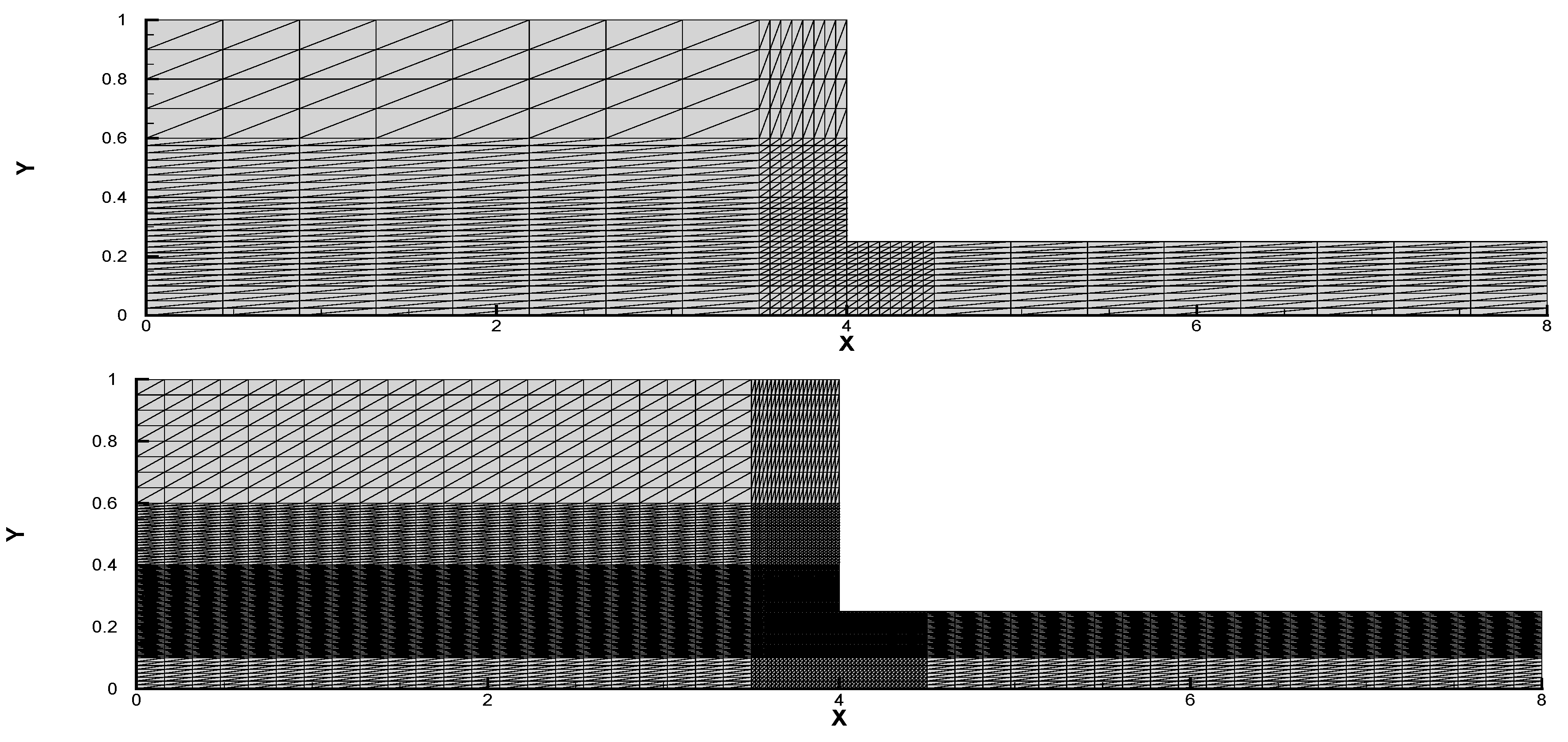
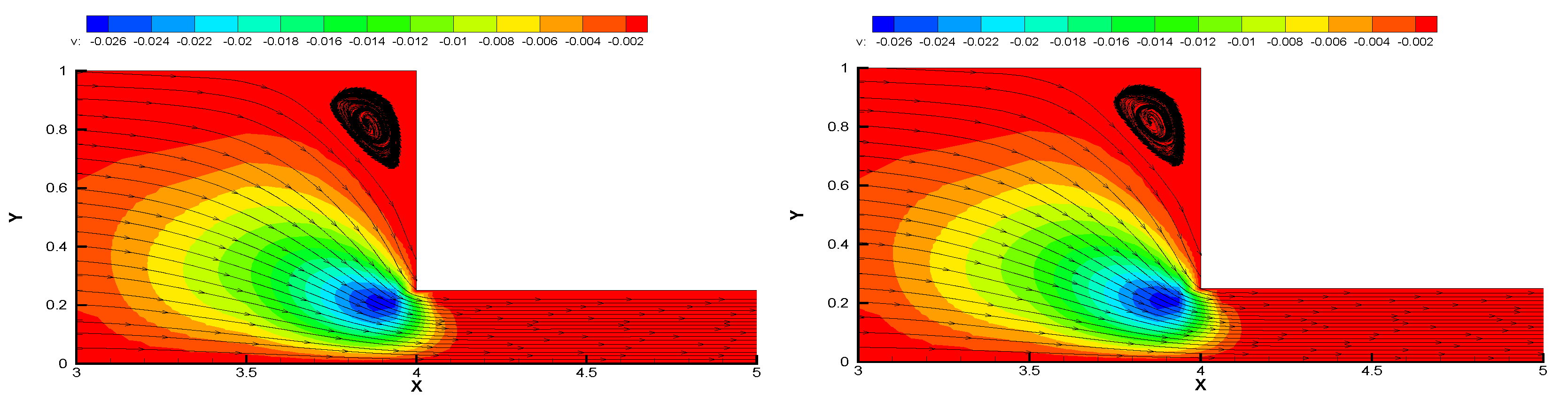
5.2. 4:1 Contraction Channel Flow

In this subsection, we examine a benchmark problem for viscoelastic fluid flow which is known as 4:1 contraction channel flow. The study of this classic reference problem is used to investigate the performance of various two-dimensional finite element, finite volume, hybrid, and spectral viscoelastic solvers. It has various interesting applications in polymeric industries. The fluid behaviour of contraction channel flow was studied widely by many authors in [35,36,37], also extensively used to show the behaviour of the streamlines and contour patterns. Here the case of planar flow through a contraction geometry with a ratio of 4:1 concerning upstream and downstream channel widths are considered. The domain is constructed such that the channel lengths are sufficiently long for fully developed Poiseuille flow at both the inflow and outflow boundaries. We demonstrate several graphical representations of viscoelastic fluid flow model and Oseen viscoelastic fluid flow behaviour for one-level and two-level method with reentrant corner flow, streamlines behaviour, pressure gradient flow behaviour. The main focus of this experiments is to illustrate the proposed algorithms efficiency, and accuracy is comparing with the well studied steady-state viscoelastic fluid flow model’s behaviour of streamlines and flow patterns.

For 4:1 contraction channel flow of Oseen viscoelastic fluid, we first determine the one-level solution of $u_1$ and $u_2$ associated with one-level contraction domain. For two-level contraction domain, the solution of $u{h}_1$ and $u{h}_2$ are determined in a similar way. We use those solutions in Oseen one-level and two-level computation as $b_1$, $b_2$, $b{h}_1$ and $b{h}_2$, respectively. The computations are performed on a uniformly refined mesh, shown in Figure 1. The method of structured mesh constructs the domain for one-level H and for two-level $h=H^{3/2}$. The one-level and two-level domain geometry consist of the vertices $(0,0),(8,0),(8,0.25),(4,0.25),(4,1),(0,1)$. The inflow and outflow boundaries are represented by $\partial {\Gamma }_{\mathrm{in}}=\{(x,y):x=0,0⩽y⩽1\}$ and $\partial {\Gamma }_{\mathrm{out}}=\{(x,y):x=8,0⩽y⩽0.25\}$ for both one-level and two-level method [27,30,31]. For the velocity,

$$\begin{array}{c}{u}_1=\frac{1}{32}(1-y^2),u_2=0,\mathrm{on}\partial {\Gamma }_{\mathrm{in}},\hfill \end{array}$$

(82)

$$\begin{array}{c}{u}_1=2(\frac{1}{16}-y^2),u_2=0,\mathrm{on}\partial {\Gamma }_{\mathrm{out}}.\hfill \end{array}$$

(83)

Figure 1. The geometry of contraction mesh for one-level (up) and two-level (down).

For stress, on $\partial {\Gamma }_{\mathrm{in}}$,

$$\begin{array}{c}{\sigma }_{11}=\frac{-\alpha \lambda (a+1){(-y/16)}^2}{(a^2-1){\lambda }^2{(-y/16)}^2-1},\hfill \end{array}$$

(84)

$$\begin{array}{c}{\sigma }_{12}={\sigma }_{21}=\frac{-\alpha (-y/16)}{(a^2-1){\lambda }^2{(-y/16)}^2-1},\hfill \end{array}$$

(85)

$$\begin{array}{c}{\sigma }_{22}=\frac{-\alpha \lambda (a-1){(-y/16)}^2}{(a^2-1){\lambda }^2{(-y/16)}^2-1}.\hfill \end{array}$$

(86)

No slip boundary conditions are imposed for the velocity on the solid walls of the contraction, and symmetry condition is imposed on the bottom of the computational domain. Besides, the physical parameters $Re$, $\alpha$, $\lambda$, and a are chosen as 1, $8/9$, $0.7$ and 1, respectively. The computation carried out using $P2-P1-P1dc$ finite elements for one-level and two-level method. The size of mesh for the 4:1 contraction channel are $0.448783$. For the one-level method, number of elements are 1408, number of nodes for $P2$ is 2945, $P1$ is 769, $P1dc$ is 4224. For the two-level method, number of elements are 12,496, number of nodes for $P2$ is 25,373, $P1$ is 6439, $P1dc$ is 37,488.

Figure 2 illustrates the graphical representation of the horizontal and vertical velocity near re-entrant corner along the vertical line $x=4.0265$ [27]. We demonstrate a one-level and two-level method for steady state viscoelastic and Oseen viscoelastic fluid flow model. From the figure, we observe that the velocity near re-entrant corner is almost continuous for one-level and two-level method. The graphical representation illustrates the flow behaviour of the horizontal velocity near re-entrant corner for one-level and two-level method is almost continuous for Oseen viscoelastic fluid and similar to the viscoelastic fluid flow. For the vertical velocity, the flow behaviour achieves a little different flow path but appear continuously. The graphical representation of the velocity near re-entrant corner shows the accuracy of the two-level scheme.

Figure 2. Horizontal velocity (left), vertical velocity (right) near re-entrant corner for steady state viscoelastic and Oseen viscoelastic fluid flow one-level and two-level method.

In the Figure 3 and Figure 4, we represent the streamlines and magnitude for steady state viscoelastic fluid flow and Oseen viscoelastic fluid flow for one-level and two-level algorithms. The figures demonstrate that the flow enters through the inflow boundary $\partial {\Gamma }_{\mathrm{in}}=\{(x,y):x=0,0⩽y⩽1\}$ and flow out through the outflow boundary $\partial {\Gamma }_{\mathrm{out}}=\{(x,y):x=8,0⩽y⩽0.25\}$. As expected, the flow behaviour of the viscoelastic type always creates a vortex in the corner [27,34]. Oseen viscoelastic fluid flow is a reduced linear model of the viscoelastic fluid flow model. The accuracy, behaviour of the streamlines, flow characteristics and the shape of the contour is examined by the Figure 3. In Figure 3, the flow pattern and nature of the streamlines are presented for the steady-state viscoelastic model and Oseen viscoelastic fluid flow model with the one-level algorithm. The contour is drawn by using the values generated for $\mathbf{v}$. The comparison of both figures for one-level method illustrates that the reduced Oseen viscoelastic fluid flow model’s shape of the contour is regular and obtains similar accuracy. The flow rate and behaviour of the streamlines are also almost same. In the Figure 4, the fluid flow behaviour of the two-level algorithm is presented for the steady-state viscoelastic model and Oseen viscoelastic fluid flow model. The contour is drawn for the two-level method with $uh$ where the red colour in the outflow channel shows the maximum flow speed. In the inflow boundary, the flow speed is less, which is represented by the contour colour and the slower flow is in the corner section where a vortex form. The shape of contour, the behaviour of the streamlines and flow rate obtain similar accuracy for the two-level method for steady state viscoelastic fluid flow and Ossen viscoelastic fluid flow. All the figures appear with similar precision, and the patterns of the streamlines are regular which validate the numerical computation’s accuracy. The physically valid results give the relevance of the numerical methods.

Figure 3. Streamlines and magnitude of velocity contours $\mathbf{u}$ for one-level method: steady state viscoelastic fluid flow (left), Oseen viscoelastic fluid model (right).

Figure 4. Streamlines and magnitude of velocity contours $\mathbf{u}$ for two-level method: steady state viscoelastic fluid flow model (left), Oseen viscoelastic fluid flow model (right).

In Figure 5, we represent the pressure contour for one-level and two-level methods for Oseen viscoelastic fluid. The figures reveal the similar pattern and no pressure oscillation which also confirm the two-level process accuracy.

Figure 5. Representation of pressure contour p: for one-level (left) and two-level (right) method for Oseen viscoelastic fluid flow.

6. Conclusions

In this contribution, the two-level decoupled method for Oseen viscoelastic fluid flow is presented and implemented for theoretical analysis with numerical experiments. Oseen viscoelastic fluid flow model is a reduced linear model of the viscoelastic fluid flow model. The proposed numerical scheme is reasonable for Oseen type problem where the non-linearity vanishes. To solve a multi-model, two-level approach is familiar with its computational flexibility. The method developed herein reduces the computational cost and implementation is easy. The solution on the coarse grid is derived in the first step, and the result is used to determine the solution on the fine mesh in the second step. The well-posedness of the scheme ensures the validation of the temporal discretization. The scaling of $h=H^{3/2}$ guarantees the linear convergence and the optimality of the convergence order is an open question. The numerical experiments support the theoretical analysis accuracy. The optimal convergence order is obtained by considering an analytical solution of the model problem. The graphs and figures of the viscoelastic fluid flow model and Oseen viscoelastic fluid flow model for the one-level and two-level methods appear in similar precision, which also validate the numerical computation accuracy. The results of the theoretical analysis and numerical simulation illustrate the algorithm proposed here can be applied to the linear Oseen type PDEs conveniently.

References

1. Oldroyd, J.G. On the formuation of rheological equations of state. Proc. R. Soc. Lond. A 1950, 200, 523–541. [Google Scholar] [CrossRef]
2. Ervin, V.J.; Lee, H.K.; Ntasin, L.N. Analysis of the Oseen-viscoelastic fluid flow problem. J. Non-Newton. Fluid Mech. 2005, 127, 157–168. [Google Scholar] [CrossRef]
3. Reed, W.H.; Hill, T.R. Triangular Mesh Methods for the Neutron Transport Equation; Tech. Report LA-UR-73-479; Los Alamos Scientific Laboratory: Los Alamos, NM, USA, 1973.
4. Lesaint, P.; Raviart, P.A. On a finite element method for solving the neutron transport equation. In Mathematical Aspects of Finite Elements in Partial Differential Equations; de Boor, C., Ed.; Academic Press: Cambridge, MA, USA, 1974; pp. 89–123. [Google Scholar]
5. Fortin, M.; Fortin, A. A new approach for the FEM simulation of viscoelastic flows. J. Non-Newton. Fluid Mech. 1989, 32, 295–310. [Google Scholar] [CrossRef]
6. Fortin, A.; Zine, A.; Agassant, J.F. Computing viscoelastic fluid flow problems at low cost. J. Non-Newton. Fluid Mech. 1992, 45, 209–229. [Google Scholar] [CrossRef]
7. Baranger, J.; Sandri, D. Finite element approximation of viscoelastic fluid flow: Existence of approximate solutions and error bounds. Numer. Math. 1992, 63, 13–27. [Google Scholar] [CrossRef]
8. Najib, K.; Sandri, D. On a decoupled algorithm for solving a finite element problem for the approximation of viscoelastic fluid flow. Numer. Math. 1995, 72, 223–238. [Google Scholar] [CrossRef]
9. Sandri, D. Finite element approximation of viscoelastic fluid flow: Existence of approximate solutions and error bounds. Continuous approximation of the stress. SIAM J. Numer. Anal. 1994, 31, 362–377. [Google Scholar] [CrossRef]
10. Ervin, V.J.; Miles, W.W. Approximation of time-dependent viscoelastic fluid flow: SUPG approximation. SIAM J. Numer. Anal. 2003, 41, 457–486. [Google Scholar] [CrossRef]
11. Ervin, V.J.; Miles, W.W. Approximation of time-dependent, multi-component, viscoelastic fluid flow. Comput. Methods Appl. Mech. Eng. 2005, 194, 2229–2255. [Google Scholar] [CrossRef]
12. Jenkins, E.; Lee, H. A domain decomposition method for Oseen-viscoelastic flow equations. Appl. Math. Comput. 2008, 195, 127–141. [Google Scholar] [CrossRef]
13. Ervin, V.J.; Lee, H. Defect correction method for viscoelastic fluid flows at high Weissenberg number. Numer. Methods Part. Differ. Equ. 2006, 22, 145–164. [Google Scholar] [CrossRef]
14. Wang, A.; Zhao, X.; Qin, P.; Xie, D. An Oseen two level stabilized mixed finite element method for the 2D/3D stationary Navier-Stokes equations. Abstr. Appl. Anal. 2012, 2012, 520818. [Google Scholar] [CrossRef]
15. Medvidova, M.L.; Mizerova, H.; Notsu, H.; Tabata, M. Numerical analysis of the Oseen-type Peterlin viscoelastic model by the stabilized Lagrange-Galerkin method Part II: A nonlinear scheme. Math. Model. Numer. Anal. SMAI 1999, 51, 1663–1689. [Google Scholar] [CrossRef]
16. Xu, J. Two-Grid discretization techniques for linear and nonlinear PDEs. SIAM J. Numer. Anal. 1996, 33, 1759–1778. [Google Scholar] [CrossRef]
17. Layton, W.; Tobiska, L. A two-level method with backtracking for the Navier-Stokes equations. SIAM J. Numer. Anal. 1998, 35, 2035–2054. [Google Scholar] [CrossRef]
18. Mu, M.; Xu, J. A two grid method of a mixed Stokes-Darcy model for coupling fluid flow with porous media flow. SIAM J. Numer. Anal. 2007, 45, 1801–1813. [Google Scholar] [CrossRef]
19. Qin, X.Q.; Dang, F.N.; Gong, C.Q. Two grid method for the characteristic mixed finite element approximations of 2D nonlinear convection diffusion problems. Chin. J. Eng. Math. 2009, 26, 906–916. [Google Scholar]
20. Yan, W.J.; Ren, C.F.; Ma, Y.C. Numerical simulation of two grid method for the unsteady Navier-Stokes equations. Chin. J. Eng. Math. 2005, 22, 1026–1030. [Google Scholar]
21. Liu, Q.F.; Hou, Y.R. A two-level finite element method for the Navier-Stokes equations based on a new projection. Appl. Math. Model. 2010, 34, 383–399. [Google Scholar] [CrossRef]
22. He, Y.N.; Wang, A. A simplified two-level method for the steady Navier-Stokes equations. Comput. Methods Appl. Mech. Eng. 2008, 197, 383–399. [Google Scholar] [CrossRef]
23. Dai, X.X.; Cheng, X.L. A two-grid method based on Newton iteration for the Navier-Stokes equations. J. Comput. Appl. Math. 2008, 220, 566–573. [Google Scholar] [CrossRef]
24. Lee, H. A multigrid method for viscoelastic fluid flow. SIAM J. Numer. Anal. 2004, 42, 109–129. [Google Scholar] [CrossRef]
25. Liakos, A.; Lee, H. Two-level finite element discretization of viscoelastic fluid flow. Comput. Methods Appl. Mech. Eng. 2003, 192, 4965–4979. [Google Scholar] [CrossRef]
26. Zhang, Y.Z.; Hou, Y.R.; Mu, B.Y. A two-grid method based on Newton iteration for viscoelastic fluid flow. Chin. J. Eng. Math. 2012, 29, 117–130. [Google Scholar]
27. Zhang, Y.; Hou, Y.; Mu, B. Defect correction method for time-dependent viscoelastic fluid flow. Int. J. Comput. Math. 2011, 88, 1546–1563. [Google Scholar] [CrossRef]
28. Baranger, J.; Wardi, S. Numerical analysis of a FEM for a transient viscoelastic flow. Comput. Methods Appl. Mech. Eng. 1995, 125, 171–185. [Google Scholar] [CrossRef]
29. Girault, V.; Raviart, P. Finite Element Methods for Navier-Stokes Equations; Springer: Berlin/Heidelberg, Germany, 1986. [Google Scholar]
30. Ervin, V.J.; Howell, J.S.; Lee, H. A two-parameter defect-correction method for computation of steady-state viscoelastic fluid flow. Appl. Math. Comput. 2008, 196, 818–834. [Google Scholar] [CrossRef]
31. Chrispell, J.C.; Ervin, V.J.; Jenkins, E.W. A fractional step θ-method approximation of time-dependent viscoelastic fluid flow. J. Comput. Appl. Math. 2009, 232, 159–175. [Google Scholar] [CrossRef]
32. Hecht, F. FreeFEM++. J. Numer. Math. 2012, 20, 251–265. [Google Scholar] [CrossRef]
33. Zheng, H.; Yu, J.; Shan, L. Unconditional error estimates for time dependent viscoelastic fluid flow. Appl. Numer. Math. 2017, 117, 1–17. [Google Scholar] [CrossRef]
34. Zhang, Y.; Hou, Y.; Yang, G. A defect-correction method for time-dependent viscoelastic fluid flow based on SUPG formulation. Discret. Dyn. Nat. Soc. 2011, 2011, 689804. [Google Scholar] [CrossRef]
35. Comminal, R.; Hattel, J.H.; Alves, M.A.; Spangenberg, J. Vortex behavior of the Oldroyd-B fluid in the 4-1 planar contraction simulated with the stream function-log-confirmation formulation. J. Non-Newton. Fluid Mech. 2016, 237, 1–15. [Google Scholar] [CrossRef]
36. Owens, R.G.; Phillips, T.N. Computational Rheology; Imperial College Press: London, UK, 2002. [Google Scholar]
37. Marchal, J.M.; Crochet, M.J. Hermitian finite elements for calculating viscoelastic flow. J. Non-Newton. Fluid Mech. 1986, 20, 187–207. [Google Scholar] [CrossRef]