Numerical Methods for a Two-Species Competition-Diffusion Model with Free Boundaries

Department of Mathematics, University of South Carolina, Columbia, SC 29208, USA
*
Author to whom correspondence should be addressed.
†
These authors contributed equally to this work.
Mathematics 2018, 6(5), 72; https://doi.org/10.3390/math6050072
Submission received: 31 March 2018
/
Revised: 27 April 2018
/
Accepted: 28 April 2018
/
Published: 3 May 2018
(This article belongs to the Special Issue Numerical Methods for Partial Differential Equations)
Abstract
:The systems of reaction-diffusion equations coupled with moving boundaries defined by Stefan condition have been widely used to describe the dynamics of spreading population and with competition of two species. To solve these systems numerically, new numerical challenges arise from the competition of two species due to the interaction of their free boundaries. On the one hand, extremely small time steps are usually needed due to the stiffness of the system. On the other hand, it is always difficult to efficiently and accurately handle the moving boundaries especially with competition of two species. To overcome these numerical difficulties, we introduce a front tracking method coupled with an implicit solver for the 1D model. For the general 2D model, we use a level set approach to handle the moving boundaries to efficiently treat complicated topological changes. Several numerical examples are examined to illustrate the efficiency, accuracy and consistency for different approaches.
1. Introduction
The reaction-diffusion equations over a changing domain to describe the dynamics of a two-species competition-diffusion model usually take the following form,
The nonlinear functions and are assumed to be functions satisfying = = 1,2, and in the literature they are often taken to be two-species Lotka-Volterra type competition functions. In the rest of this paper, we will take two-species Lotka-Volterra type competition functions as an example to demonstrate the numerical methods.
The evolution of the moving domains , or rather their boundaries = 1,2 is determined by the one phase Stefan condition which, in the case are manifolds in . For example, the evolution of species U can be described as follows:
- For any point , it moves with velocity , where is the unit outward normal of at , and is a given positive constant.
The moving boundaries is generally called the “free boundary”, and it is well known that, in general, their smoothness is not guaranteed, even if the initial function , and initial domain are both smooth.
Mathematically, the two-species competition-diffusion model with two free boundaries has been intensively studied for 1D [1,2,3,4] and for high dimensions with radial symmetry [5,6] through profound mathematical analysis. For instance, the existence of the positive traveling wave solutions connecting different constant equilibria has been addressed in [7,8,9]. The asymptotic spreading speed associated with the Cauchy problem has been studied in [10,11,12]. Many other theoretical results for general models have been achieved in [13,14,15,16,17] and references cited therein.
In contrast, very few numerical methods have been developed to solve such free boundary problems. Most recently, some efficient numerical methods have been introduced to solve the single species model [18]. In general, extremely small time steps are required due to the stiffness of the system. On the other hand, it is always difficult to efficiently and accurately handle the moving boundaries especially for two species. To efficiently handle the moving boundaries, level set methods [19,20,21,22,23,24] and front tracking methods [25,26,27,28] are two popular numerical approaches. One distinct feature of front tracking [29,30,31,32,33,34] is using a pure Lagrangian approach to explicitly track locations of interfaces, but it is difficult to handle topological bifurcations in high dimensions with interaction of two free boundaries, while the level set method can efficiently overcome such difficulties. In this paper, we will introduce a front tracking framework to solve the system for the one-dimensional case, and a level set approach is employed for two dimensions.
The rest of paper is organized as follows. In Section 2, we introduce two approaches for one-dimensional two-species competition system , i.e., a front tracking approach and a front fixing approach. In Section 3, a level set method is discussed for a more general two-dimensional case. In Section 4, numerical examples are performed to show the efficiency, accuracy and consistency for these different approaches. Finally, a brief conclusion is drawn in Section 5.
2. Numerical Methods for 1D Two-Species Competition-Diffusion Model
A two-species competition-diffusion model with two free boundaries for the density of population of the competing species U and V depending on time t and spatial variable x states as follows:
where and represent the population densities of the two species at the position x and time t. and are the diffusion rates of species U and V. and are net birth rates of species U and V. and are the competition coefficients of species U and V. The parameters and measure the intention to spread into the new territories of u and v. Here, the two free boundaries and describe the spreading fronts of two competing species and . We envision that the two species initially occupy the interval and , respectively, at time t.
2.1. Method 1: Front-Tracking Method for 1D Two-Species Competition-Diffusion Model
The problem lies in solving the nonlinear parabolic partial differential Equations (3)–(9) in the unbounded fixed domain for the variables . Let us consider the step size discretization , , and the mesh points , with and M positive integer. Let us denote the approximate value of and the approximate value of at the mesh point ,
Step1: Track the position of the moving front .
According to the Stefan condition
we consider using the central approximation of the spatial derivatives to approximate , which can be divided into the following four cases.
- 1
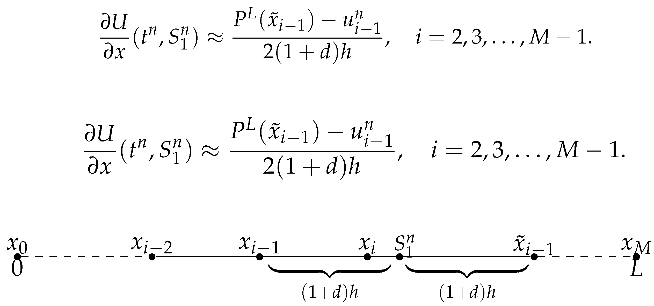
- When as depicted in Figure 1, denoting . Let us first consider the symmetric point of respect to the position , which is denoted by . In particular, when , . We use the Lagrange interpolation to construct polynomial from the value of d, h, , , and , thus at , we use the value of at instead of ,
- 2
- When , the central scheme approximation of the spatial derivatives to approximate involves the fictitious value at the point . The value can be estimated from the second-order discretization of the boundary condition (10),which implies that . It is obvious that all the values of on the grid points are equal to 0 except . Numerically, we take , and this can be explained by the fact the species is only located inside one grid mesh. The simulation should stop here indicating that a more refined mesh is needed.
- 3
- When as shown in Figure 2, denoting . Let us first consider the symmetric point of with respect to the position , which is denoted by . Then we consider the value of , and use the Lagrange interpolation to construct polynomial from the value of h, d, , , and . Then at , we use the value of at instead of .
- 4
- When , it implies that the spreading of the populations already goes out of the computational domain , and the simulation should stop here.
Step2: Track the position of the moving front of .
Repeat step1 to .
Step3: Update the value of and .
- 1
- When and , then we know that . Let , , for and , , for . We consider the central approximation of the spatial derivatives at , for , and the central approximation of the spatial derivatives at , for , where U and V are updated by the backward EulerThen use the Iteration (or Newton Iteration) to solve the nonlinear system (12).
- 2
- When and , denoting and , we use the Lagrange interpolation to construct polynomial from the value of h, , , , and and polynomial from the value of h, , , , and . Then at and , we use the value of at instead of and the value of at instead of . For the solution u at , for , a standard central approximation in space with backward Euler in time will be employed. , for . For the solution v at , for , a standard central approximation in space with backward Euler in time will be employed. , for . U and V is updated by the backward Euler in timeIteration (or Newton Iteration) will be applied to solve the nonlinear system (13).
- 3
- When and , then we know that . Let , , for . We consider the central approximation of the spatial derivatives at , for . Denoting , we use the Lagrange interpolation to construct polynomial from the value of h, , , , and . Then at , we use the value of at instead of , where U and V is updated by the backward Euler in timeThen use the Iteration (or Newton Iteration) to solve the nonlinear system (14).
- 4
- When and , denoting , we use the Lagrange interpolation to construct polynomial from the value of h, , , , Then at , we use the value of at instead of . For the solution u at , for , a standard central approximation in space with backward Euler in time will be employed. , for . For the solution v at , for , a standard central approximation in space with backward Euler in time will be employed. , for , where U and V is updated by the backward Euler in timeIteration (or Newton Iteration) will be applied to solve the nonlinear system (15).
2.2. Method 2: Front-Fixing Method for 1D Two-Species Competition-Diffusion Model
Here we consider transforming Equation (3) and Equation (4) into problems with a fixed domain separately.
Step1. Update the front of and the value of U by front fixing method.
Let us transform Equation (3) into a problem with a fixed domain using the Landau transformation [35,36]
Boundary conditions (5) and Stefan condition (6) take the form:
and
respectively, while the initial conditions (9) become:
Conditions (8) for the initial function are translated to as follows:
After the transformation, the new problem has been changed to solve the nonlinear parabolic partial differential equations (17) in the unbounded fixed domain for the variables . Let us consider the step size discretization , , and the mesh points , with and M positive integer. Let us denote the approximate value of at the mesh point ,
and let be the approximation of . Let us consider the forward approximation of the time derivatives,
and the central approximation of the spatial derivatives,
As usual, we assume that the Equation (26) can be also approximated at . Equation (26) written for involves the fictitious value at the point . The value is eliminated from the discretization of the boundary and initial condition (21) and (22),
Transformed Stefan condition (20) is discretized using first order forward approximation for and three points backward spatial approximation of :
to preserve accuracy of order .
Finally, we have
where the coefficients are given by:
Step2. Update the front and the value of V by front fixing method.
Let us transform Equation (4) into a problem with a fixed domain using the Landau transformation [35,36]
Then Equation (4) turns into the form:
where:
Boundary conditions (5) and Stefan condition (6) take the form:
and
respectively, while the initial conditions (9) become:
Conditions (8) for the initial function are translated to as follows:
After the transformation, the new problem lies in solving the nonlinear parabolic partial differential equations (31) in the unbounded fixed domain for the variables . Let us consider the step size discretization , , and the mesh points , with and M positive integer. Let us denote the approximate value of at the mesh point ,
and let be the approximation of . Let us consider the forward approximation of the time derivatives,
and the central approximation of the spatial derivatives,
As usual, we again assume that Equation (40) can be also approximated at . Equation (40) written for involves the fictitious value at the point . The value is eliminated from the discretization of the boundary and initial condition (35) and (36),
Transformed Stefan condition (34) is discretized using first order forward approximation for and three points backward spatial approximation of :
to preserve accuracy of order .
Finally, we have
where the coefficients are given by:
Step3. Update the value of with the front information and .
- 1
- When , then we know that . Let , , for . We consider the central approximation of the spatial derivatives at , for , where is updated by the backward Euler
- 2
- When , denoting , we use the Lagrange interpolation to construct polynomial from the value of h, R, , , and , We consider to use the value of at instead of .
- 3
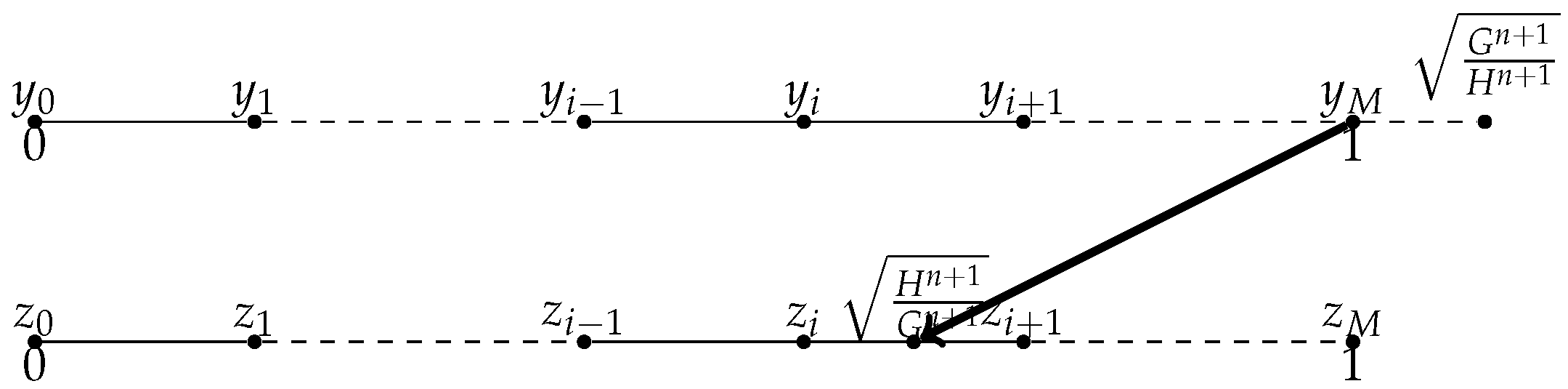
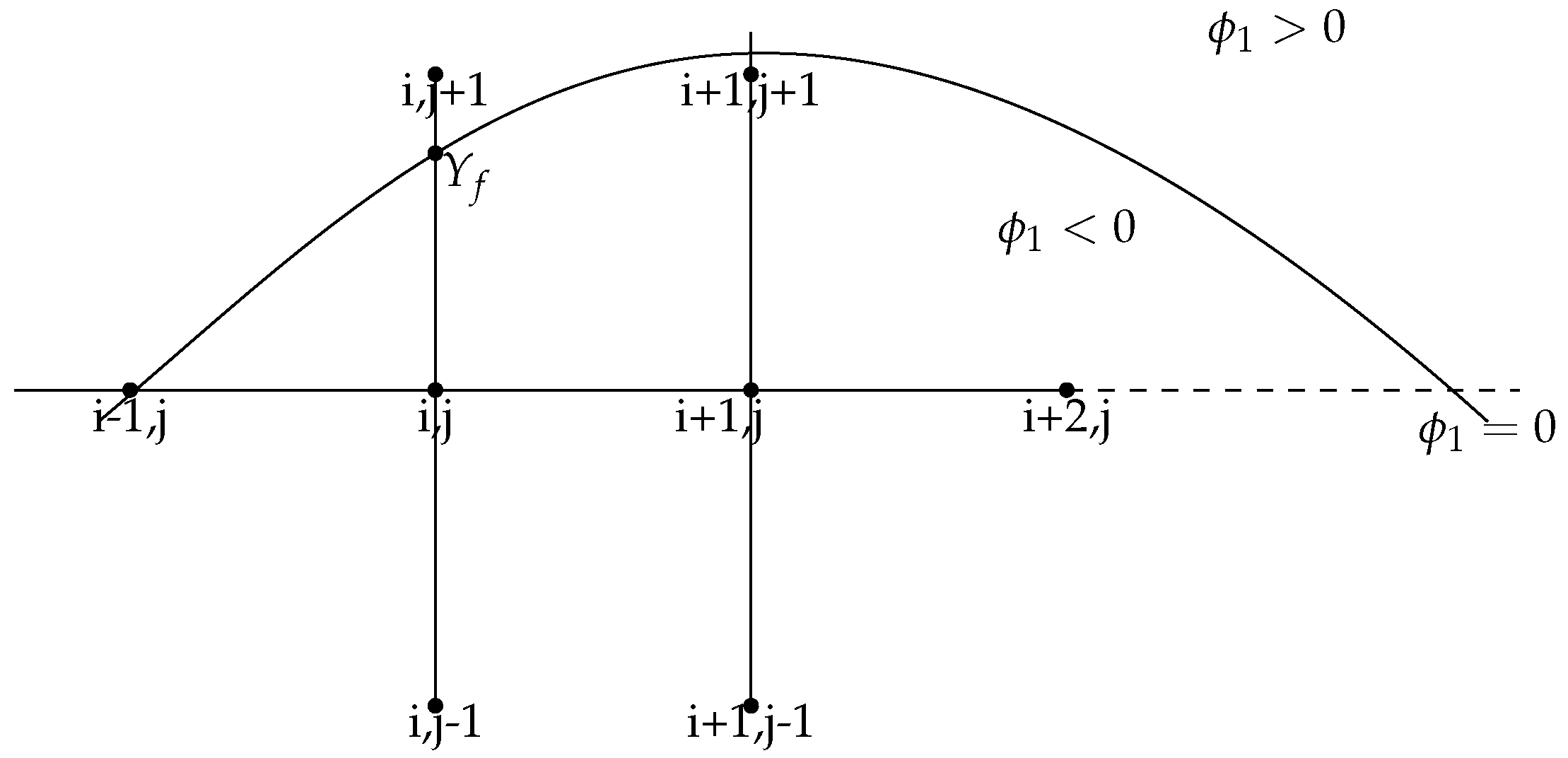
- When as shown in Figure 3, we consider the central approximation of the spatial derivatives at , for , for , we know that , let us approximate instead of approximating . Suppose , we use the Lagrange interpolation to construct polynomial P from the value of , , , , , and , then .
Step4. Update the value of with the front information and .
- 1
- When , then we know that . Let , , for . We consider the central approximation of the spatial derivatives at , for , where M is updated by the backward Euler
- 2
- When , denoting , we use the Lagrange interpolation to construct polynomial from the value of h, R, , , and , We consider to use the value of at instead of .
- 3
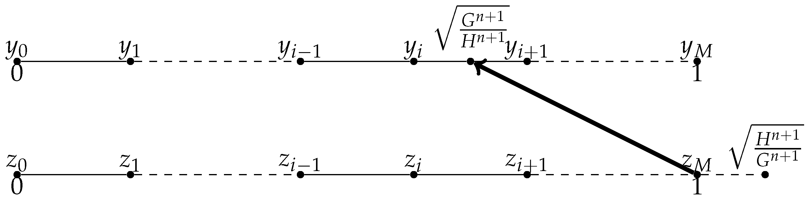
- When as illustrated in Figure 4, we consider the central approximation of the spatial derivatives at , for , for , we know that , let us approximate instead of approximating . Suppose , we use the Lagrange interpolation to construct polynomial P from the value of , , , , , and , then .
3. Level Set Method for 2D Two-Species Competition-Diffusion Model
A general 2D two-species competition-diffusive model for the densities of population of the species and depending on time t and spatial variable states as follows:
together with the boundary conditions
the Stefan conditions
where and are, respectively, the velocity vector of the boundary point , and the unit outward normal of at , and are, respectively, the velocity vector of the boundary point , and the unit outward normal of at , and the initial conditions
The initial functions and satisfies the following properties:
Here and are the unknown moving boundaries of two species and such that the population are distributed in the domain and separately. and are the dispersal rates. The parameters and involved in the Stefan conditions (51) and (52) are the proportionality constant between the population gradient at the front and the speed of the moving boundary of two species and respectively. Following the ideas of [19], here we use a level set approach to effectively capture the front at each new time step and a finite difference scheme to solve the heat equation everywhere away from the front. The idea behind the level set method is to construct a level set function , then move with the correct speed at the front and followed by updating . The new position of the front is stored implicitly in . With this approach, we avoid the difficulties that arise from explicitly tracking the front and thus increase the efficiency to deal with complex interfacial geometries.
Step1. Initialize and .
We construct a level set function , such that at any time t, the front is equal to the zero level set of , i.e.,
Initially, and is set equal to the signed distance function from the front of species U such that is negative in and positive in ,
where d is the distance from the front .
Given the normal speed, , at which the front moves, we would construct a speed function, , which is a continuous extension of from the front over the whole computational domain. The governing equation of is then given by
This equation will move with the correct speed at the front by assuring that will always coincide with the zero level set of at time t.
We also use to define the outward normal vector corresponding to by
Since is equal to along the interface, we can combine Equations (58) and (60) to get the following equation, which of course is only valid on the zero level set of :
Next, we need to extend the velocity function to a neighborhood of .
Therefore, we get the velocity function over the computational domain
which is of course only valid on the zero level set of .
Step2. Compute the velocity filed of U .
By introducing defined as an extension of from , we can avoid unnecessary numerical difficulties when we solve Equations (60) and (61).
One issue in computing arises from the fact that its approximation is usually in the order at points close to or on the front.
The approximation to at is based upon approximations to the derivatives of U in four coordinate directions to cut down on grid orientation effects (please see Figure 5 for illustration). Each approximation to a derivative of U can be continuously extended away from the front by the advection equations
where , , and on . Here S is equal to the sign function. Equation (64) through Equation (67) have the effect of continuously extending away from the front by advecting these fields in the proper upwind direction. Note that these equations will not degrade the value of on the front because is zero on , hence, so are , , and .
From (63), we end up solving for the right hand side of the equation
The spatial first derivatives of are approximated by a second-order ENO scheme. We update by solving (68) with a third-order Runge-Kutta scheme.
Step3: Update to be a signed distance function for one time step.
From Equation (58) and (59), it is clear that the computation of the normal velocity, and normal vector at the front are all dependent upon the level set function . However, by Equation (58), the level set function will cease to be an exact distance function even after one time step. In order to keep the accuracy of , and , we need to avoid having steep or flat gradients developed in . One way to avoid these numerical difficulties is to reinitialize to be an exact distance function from the evolving front at each time step.
In order to reinitialize the level set function, we use the reinitialization scheme of Sussman [37]
where and S again denotes the sign function. As in [37], the sign function S is smoothed by the equation.
The basic idea behind this method is that given a function that is not a distance function, one can evolve it into a function that is an exact signed distance function from the zero level set of . This can be accomplished by iterating (69) to a steady state. As in [37], the sign function S is smoothed by the equation
to avoid numerical difficulties while implemented.
By using this approach, we avoid having to explicitly find the contour and then resetting values of the front at grid points. From Equation (69), it is clear that the original position of the front will not change, but at points away from , will be evolved into a distance function.
Step4: Update .
After moving by the correct velocity at the front and then reinitializing to be an exact signed distance function from in Step 3, next we update . Updating essentially boils down to solving the nonlinear parabolic partial difference equation (48) over the whole computational domain in the following three cases:
- At points away from the front, which means the nearby four grid points are all inside the domain , we solve the nonlinear parabolic partial difference equation (53) by combining the forward Euler method and the five-point stencil scheme.
- For points near the front , some special care should be taken. We effectively capture the front using the level set function . We can use the one-sided different sign of to incorporate the distances between a point on the front and grid points neighboring it in either the vertical or horizontal direction. For example, , we consider two grid points and which border . In y-direction, we have . We introduceand use and to construct interpolating polynomial P. When updating , we use a standard five-point stencil combing forward Euler method by employing instead of , i.e.,For the case when front interacts with x-axis, we use the same process in x-direction. In the special case where we cannot find enough grid points inside the domain to construct interpolating polynomial P, we employ the nearby grid points and intersect points of the front and x and y-axis to construct quadratic polynomial or straight line as the interpolating polynomial P to update U. For the extreme configuration, where there are only intersect points of the front and x and y-axis near the grid point, we update at the grid point.
- If a grid point lies on the front, we set the value at that point (in view of (53)). For example, we set =0 for the grid point .
Step5. Repeat Step 2 through Step 4 to and .
Step6. Repeat Step 2 through Step 6 to update , , U and V for the next time step.
4. Numerical Experiments
4.1. Numerical Tests of 1D Problem: Front-Fixing Method and Front-Tracking Method
Convergence test of front-fixing method
In the 1D two-species competition-diffusion model (3)–(9) with parameters values = , = , , and . Here we test the order of convergence in space with very refined temporal step size.
In Table 1 and Table 2 the error (both and ) and the convergence to the solution of front-fixing method is examined, with final time . The error is computed by the difference of the numerical solution with the exact solution. For all the examples below when the exact solution is not given, the solution with a very fine resolution will be considered as reference or “exact" solution. As expected, a second-order convergence in space for both u and v can be observed.
Convergence test of front-tracking method
In the 1D two-species competition-diffusion model (3)–(9) with parameters values = , = , , , and . Here we test the order of convergence in space with very refined temporal step size.
In Table 3 and Table 4 the error (both and ) and the convergence to the solution of front-tracking method is examined, with final time . The error is computed by the difference of the numerical solution with the exact solution. For all the examples below, when the exact solution is not given, the solution with a fine resolution will be considered as reference or “exact” solution. As expected, a second-order convergence in space for both u and v can be observed.
The Comparison of Front-fixing with Front-tracking for 1D model
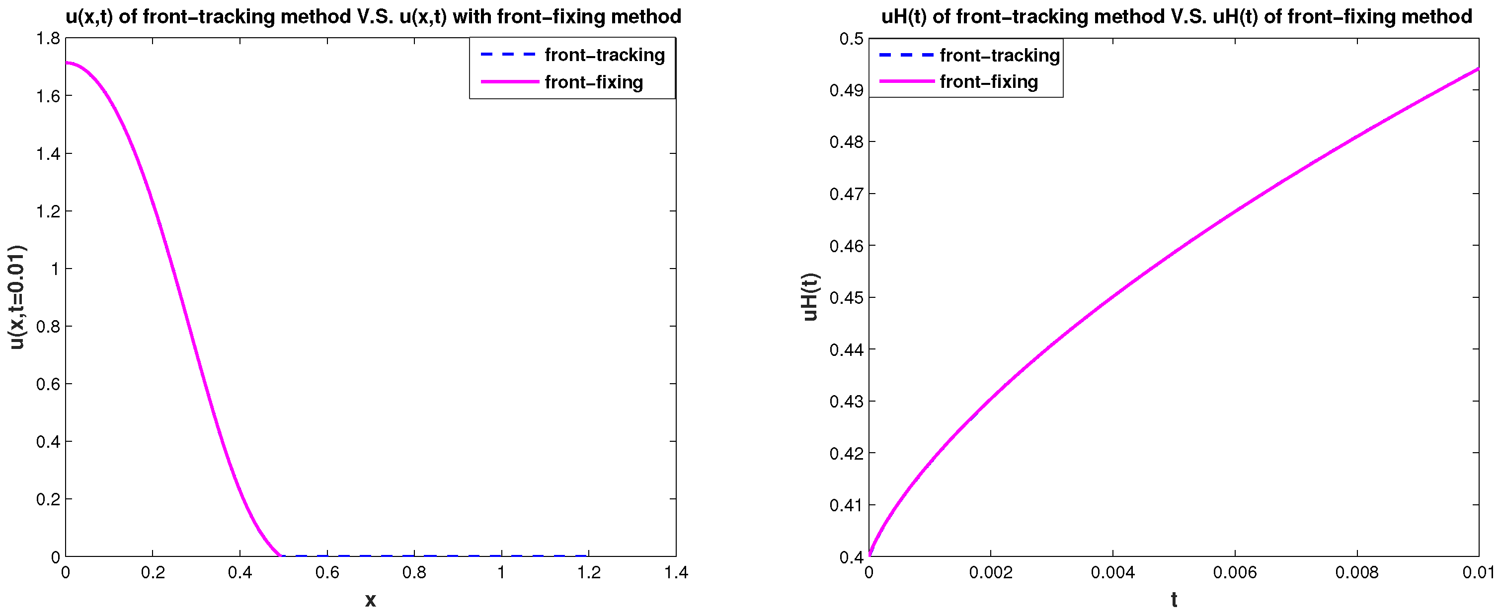
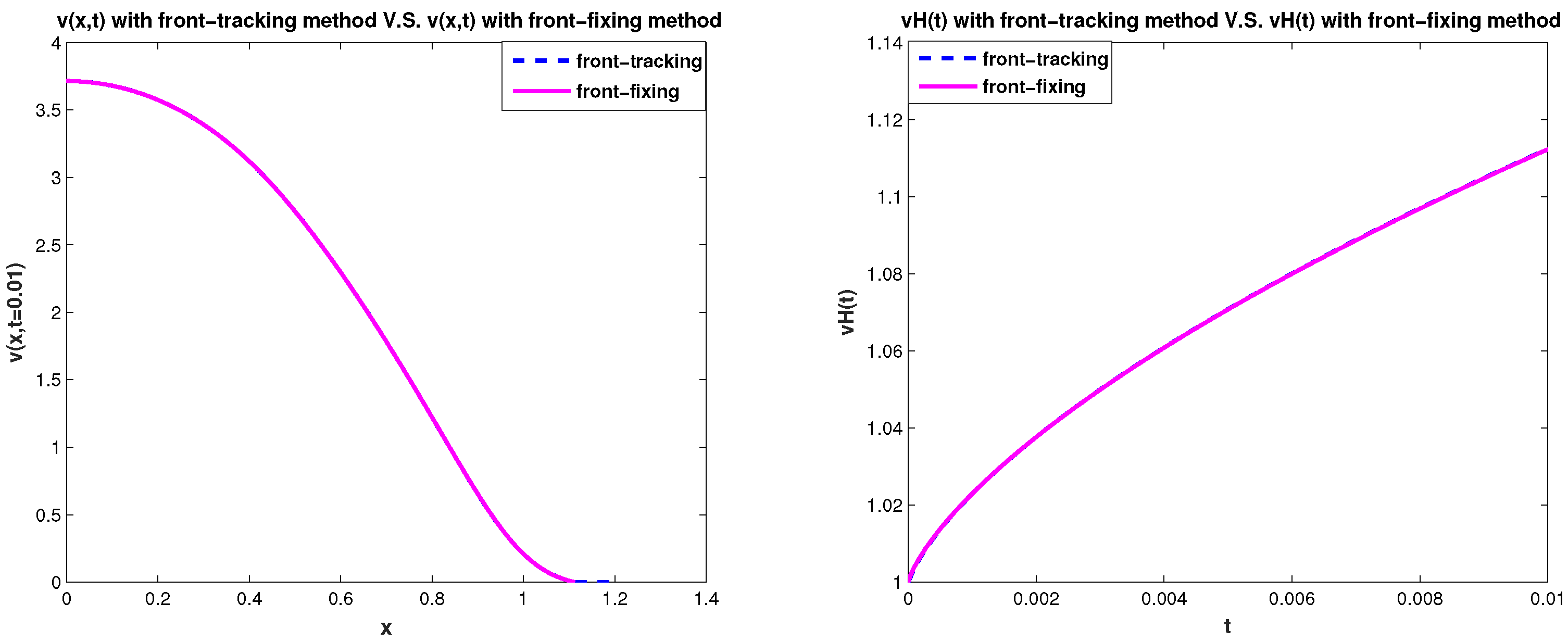
In Figure 7 and Figure 8, we use the front-fixing method and front-tracking method to simulate the 1D two-species competition-diffusion model (3)–(9) with parameters values = , = , , and and spatial size . It shows that the results of front-tracking method and the results of front-fixing method are consistent with each other.
4.2. Numerical Tests of Level Set Methods for 2D Model With Different Initial Configuration
Example 1.
In the 2D two-species competition-diffusion model (48)–(56) with parameters values = , = , the initial boundary of species U is set to be an equilateral triangle which centers at the origin point with side length 1, while the initial boundary of species V is set to be a circle which centers at the origin point with radius = 1.5. The initial values , (x,y) and the initial level set functions , (x,y) are set as follows
Figure 9 shows the simulation of the evolvement of two species and their moving boundaries along time with an equilateral triangle as the initial boundary of U and a circle as the initial boundary of V. In the figure of boundary line, the red curves represent the initial boundaries, and the blue curves simulate the evolvement of free boundaries.
From Figure 9, we can see that the triangle evolves into a circle during the simulation.
Example 2.
In the 2D two-species competition-diffusion model (48)–(56) with parameters values = , = , the initial boundary of species U is set to be a square with side length = 1, centered at (0,0), while the initial boundary of species V is set to be a circle which centers at the origin point with radius = 2. The initial values , (x,y) and the initial level set functions , (x,y)are set as following
Figure 10 shows the simulation of the evolvement of two species and their moving boundaries along time with a square as the initial boundary of U and a circle as the initial boundary of V. In the figure of boundary line, the red curves represent the initial boundaries, and the blue curves simulate the evolvement of free boundaries.
From Figure 10, we can see that the square evolves into a circle during the simulation.
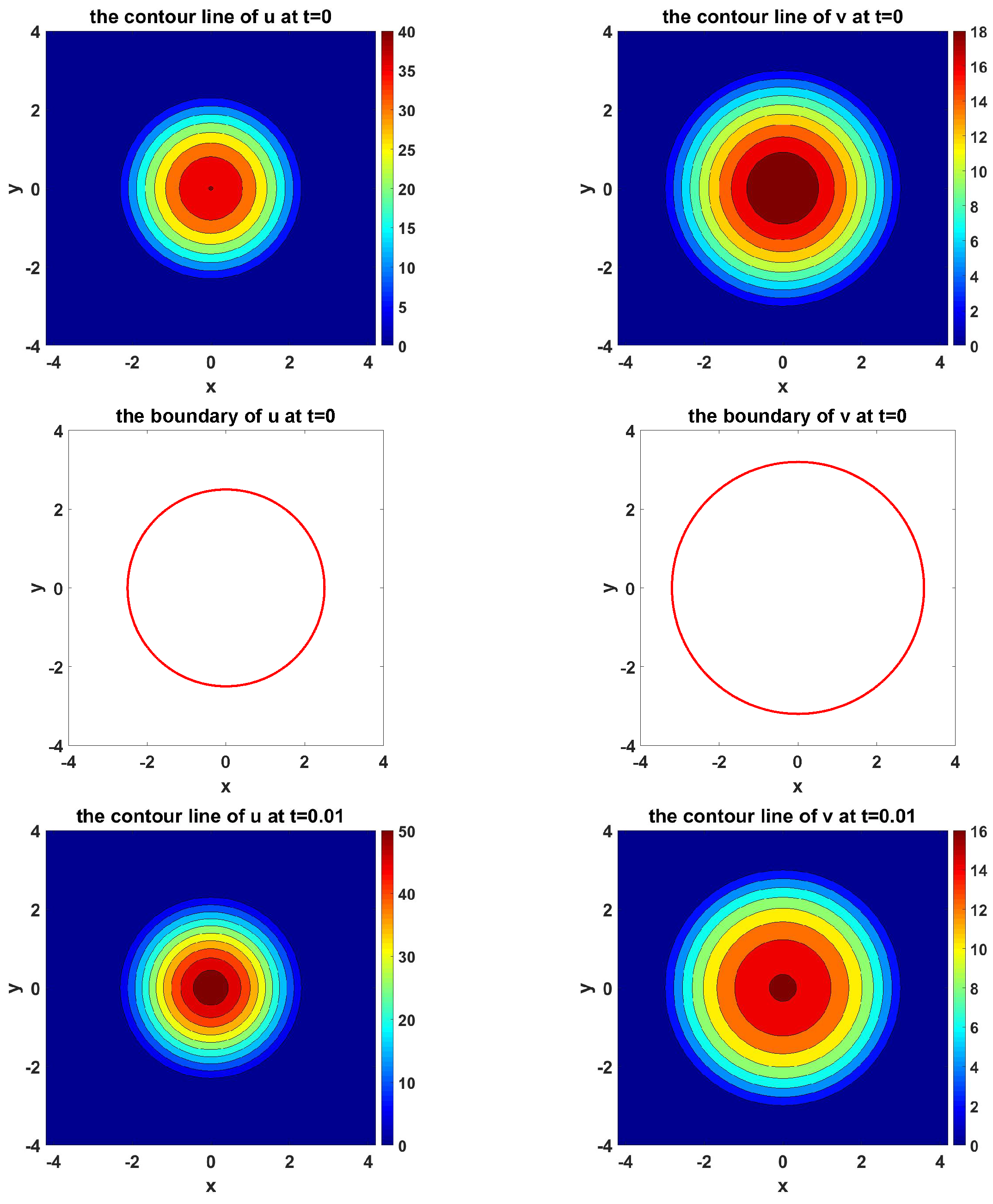
Example 3.
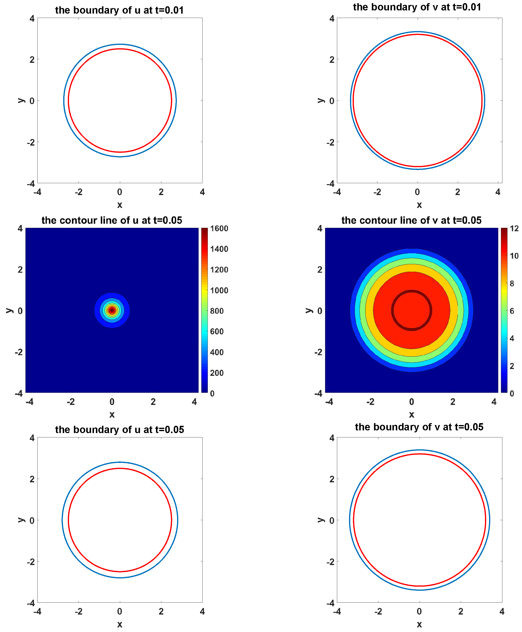
In the 2D two-species competition-diffusion model (48)–(56) with parameters values = , = , the initial boundary of species U is set to be a circle which centers at with radius = 2.5, while the initial boundary of species V is set to be a circle which centers at the origin point with radius = 3.2. The initial values , (x,y) and the initial level set functions , (x,y)are set as follows
Figure 11 shows the simulation of the evolvement of two species and their moving boundaries along time with circles as the initial boundary of U and V. In the figure of boundary line, the red curves represent the initial boundaries, and the blue curves simulate the evolvement of free boundaries.
From Figure 11, we can see that the circles propagate as circles during the simulation.
5. Conclusions
The system of reaction-diffusion equations with moving boundaries has been intensively studied analytically in recent years, however, very little numerical work has been done in this field due to numerical challenges in tracking free boundaries. In this paper, we first introduce a front tracking framework for 1D model, and compare it with a front-fixing method. Numerical experiments demonstrate that these two methods are consistent with each other. For 2D models, to overcome the difficulty of handling complicated topologically changes, we apply a level set approach to handle the moving boundaries. Numerical examples with different initial configurations demonstrate that the level set approach is able to robustly and efficiently capture different complicated geometries.
Although the level set method is very robust in handling topological changes, sometimes it is very hard to achieve high order accuracy, especially near the fronts. Currently we are extending the front tracking method to more accurately deal with topological changes for general 2D models, and to the systems of two competing species in which each species has its own moving boundary. The front will become more complicated and more challenging once two moving fronts are tangled together, and we would apply the reconstruction strategy to overcome these difficulties.
Author Contributions
X.L. and S.L. proposed and designed the numerical methods and S.L. performed the numerical experiments. X.L. and S.L. together wrote the paper.
Conflicts of Interest
The authors declare no conflict of interest.
References
- Wang, M.; Zhang, Y. Note on a two-species competition-diffusion model with two free boundaries. Nonlinear Anal. Theory Methods Appl. 2017, 159, 458–467. [Google Scholar] [CrossRef]
- Guo, J.S.; Wu, C.H. Dynamics for a two-species competition—Diffusion model with two free boundaries. Nonlinearity 2014, 28, 1. [Google Scholar] [CrossRef]
- Guo, J.S.; Wu, C.H. On a free boundary problem for a two-species weak competition system. J. Dyn. Differ. Equ. 2012, 24, 873–895. [Google Scholar] [CrossRef]
- Wu, C.H. The minimal habitat size for spreading in a weak competition system with two free boundaries. J. Differ. Equ. 2015, 259, 873–897. [Google Scholar] [CrossRef]
- Hilhorst, D.; Iida, M.; Mimura, M.; Ninomiya, H. A competition-diffusion system approximation to the classical two-phase Stefan problem. Jpn. J. Ind. Appl. Math. 2001, 18, 161. [Google Scholar] [CrossRef]
- Wang, M.; Zhao, J. Free boundary problems for a Lotka-Volterra competition system. J. Dyn. Differ. Equ. 2014, 26, 655–672. [Google Scholar] [CrossRef]
- Hosono, Y. The minimal speed of traveling fronts for a diffusive Lotka-Volterra competition model. Bull. Math. Biol. 1998, 60, 435–448. [Google Scholar] [CrossRef]
- Conley, C.; Gardner, R. An Application of the Generalized Morse Index to Travelling Wave Solutions of a Competitive Reaction-Diffusion Model; Technical Report; Wisconsin Univ-Madison Mathematics Research Center: Madison, WI, USA, 1980. [Google Scholar]
- Gardner, R.A. Existence and stability of travelling wave solutions of competition models: A degree theoretic approach. J. Differ. Equ. 1982, 44, 343–364. [Google Scholar] [CrossRef]
- Lewis, M.A.; Li, B.; Weinberger, H.F. Spreading speed and linear determinacy for two-species competition models. J. Math. Biol. 2002, 45, 219–233. [Google Scholar] [CrossRef] [PubMed]
- Li, B.; Weinberger, H.F.; Lewis, M.A. Spreading speeds as slowest wave speeds for cooperative systems. Math. Biosci. 2005, 196, 82–98. [Google Scholar] [CrossRef] [PubMed]
- Weinberger, H.F.; Lewis, M.A.; Li, B. Analysis of linear determinacy for spread in cooperative models. J. Math. Biol. 2002, 45, 183–218. [Google Scholar] [CrossRef] [PubMed]
- Du, Y.; Guo, Z. The Stefan problem for the Fisher–KPP equation. J. Differ. Equ. 2012, 253, 996–1035. [Google Scholar] [CrossRef]
- Dong, X.; Li, H.; Derdowski, A.; Ding, L.; Burnett, A.; Chen, X.; Peters, T.; Dermody, T.; Woodruff, E.; Wang, J.; et al. AP-3 directs the intracellular trafficking of HIV-1 Gag and plays a key role in particle assembly. Cell 2005, 120, 663–674. [Google Scholar] [CrossRef] [PubMed]
- Du, Y.; Lou, B. Spreading and vanishing in nonlinear diffusion problems with free boundaries. J. Eur. Math. Soc. 2015, 17, 2673–2724. [Google Scholar] [CrossRef]
- Du, Y.; Lou, B.; Zhou, M. Nonlinear diffusion problems with free boundaries: convergence, transition speed, and zero number arguments. SIAM J. Math. Anal. 2015, 47, 3555–3584. [Google Scholar] [CrossRef]
- Du, Y.; Matano, H.; Wang, K. Regularity and asymptotic behavior of nonlinear Stefan problems. Arch. Ration. Mech. Anal. 2014, 212, 957–1010. [Google Scholar] [CrossRef]
- Liu, S.; Du, Y.; Liu, X. Numerical methods for a class of reaction-diffusion equations with free boundaries. 2018; preprint. [Google Scholar]
- Osher, S.; Fedkiw, R. Level Set Methods and Dynamic Implicit Surfaces; Springer Verlag: Berlin, Germany, 2002. [Google Scholar]
- Osher, S.; Sethian, J. Fronts propagating with curvature-dependent speed: Algorithms based on Hamilton-Jacobi formulations. J. Comput. Phys. 1988, 79, 12–49. [Google Scholar] [CrossRef]
- Sethian, J. A fast marching level set method for monotonically advancing fronts. Proc. Natl. Acad. Sci. USA 1996, 93, 1591–1595. [Google Scholar] [CrossRef] [PubMed]
- Sethian, J.A. Level Set Methods and Fast Marching Methods; Cambridge University Press: Cambridge, UK, 1999. [Google Scholar]
- Xu, J.; Li, Z.; Lowengrub, J.; Zhao, H. A level-set method for interfacial flows with surfactant. J. Comput. Phys. 2006, 212, 590–616. [Google Scholar] [CrossRef]
- Zhao, H.; Chan, T.; Merriman, B.; Osher, S. A variational level set approach to multiphase motion. J. Comput. Phys. 1996, 127, 179–195. [Google Scholar] [CrossRef]
- Leveque, R.; Li, Z. The immersed interface method for elliptic equations with discontinuous coefficients and singular sources. SIAM J. Numer. Anal. 1994, 31, 1019–1044. [Google Scholar] [CrossRef]
- Peskin, C. The immersed boundary method. Acta Numer. 2003, 11, 479–517. [Google Scholar]
- Wiegmann, A.; Bube, K. The immersed interface method for nonlinear differential equations with discontinuous coefficients and singular sources. SIAM J. Numer. Anal. 1998, 35, 177–200. [Google Scholar] [CrossRef]
- Zhu, L.; Peskin, C. Simulation of a flapping flexible filament in a flowing soap film by the immersed boundary method. J. Comput. Phys. 2002, 179, 452–468. [Google Scholar] [CrossRef]
- Chern, I.; Glimm, J.; McBryan, O.; Plohr, B.; Yaniv, S. Front tracking for gas dynamics. J. Comput. Phys. 1986, 62, 83–110. [Google Scholar] [CrossRef]
- Glimm, J.; Li, X.; Liu, Y.; Zhao, N. Conservative front tracking and level set algorithms. Proc. Natl. Acad. Sci. USA 2001, 98, 14198–14201. [Google Scholar] [CrossRef] [PubMed]
- Hilditch, J.; Colella, P. A front tracking method for compressible flames in one dimension. SIAM J. Sci. Comput. 1995, 16, 755–772. [Google Scholar] [CrossRef]
- Hua, J.; Stene, J.; Lin, P. Numerical simulation of 3D bubbles rising in viscous liquids using a front tracking method. J. Comput. Phys. 2007, 227, 3358–3382. [Google Scholar] [CrossRef]
- LeVeque, R.; Shyue, K. Two-dimensional front tracking based on high resolution wave propagation methods. J. Comput. Phys. 1996, 123, 354–368. [Google Scholar] [CrossRef]
- Unverdi, S.; Tryggvason, G. A front-tracking method for viscous, incompressible, multi-fluid flows. J. Comput. Phys. 1992, 100, 25–37. [Google Scholar] [CrossRef]
- Crank, J. Free and Moving Boundary Problems; Oxford Science Publications: Oxford, UK, 1984. [Google Scholar]
- Landau, H.G. Heat conduction in a melting solid. Q. Appl. Math. 1950, 8, 81–94. [Google Scholar] [CrossRef]
- Sussman, M.; Smereka, P.; Osher, S. A level set approach for computing solutions to incompressible two-phase flow. J. Comput. Phys. 1994, 114, 146–159. [Google Scholar] [CrossRef]
Figure 1.
case 1: .

Figure 2.
case 3: .

Figure 3.
when , .

Figure 4.
when , .

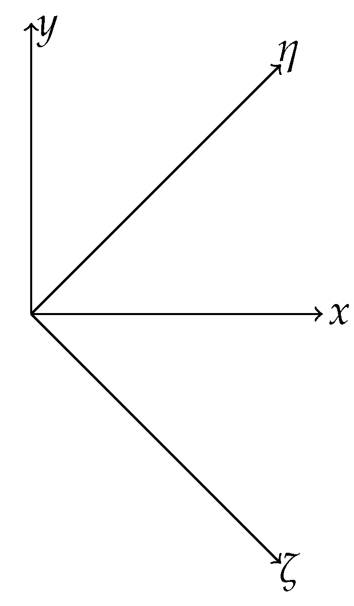
Figure 5.
Four coordinate directions used to compute the normal velocity.

Figure 6.
Illustration of updating U.

Figure 7.
u(x,t=0.01) and uH(t):Front-tracking method vs. front-fixing method for 1D model.

Figure 8.
v(x,t=0.01) and vH(t):Front-tracking method vs. front-fixing method for 1D model.

Figure 9.
The simulated dynamics where initial boundary of U is an equilateral triangle and initial boundary of V is a circle. The snapshots are taken at the times , respectively.
Figure 9.
The simulated dynamics where initial boundary of U is an equilateral triangle and initial boundary of V is a circle. The snapshots are taken at the times , respectively.

Figure 10.
The simulated dynamics where initial boundary of U is a square and initial boundary of V is a circle. The snapshots are taken at the times , respectively.
Figure 10.
The simulated dynamics where initial boundary of U is a square and initial boundary of V is a circle. The snapshots are taken at the times , respectively.

Figure 11.
The simulated dynamics where initial boundaries of U and V are circles. The snapshots are taken at the times , respectively.
Figure 11.
The simulated dynamics where initial boundaries of U and V are circles. The snapshots are taken at the times , respectively.


Table 1.
Convergence analysis of the value of U and the front of U using the front-fixing method.
| Order | Order | |||
|---|---|---|---|---|
| Accuracy test of U of front-fixing method | ||||
| 101 × | 1.195× | 2.119× | ||
| 201 | 3.142 | 1.93 | 5.424 | 1.97 |
| 401 | 8.233 | 1.93 | 1.314 | 2.05 |
| 801 | 1.956 | 2.07 | 3.983 | 1.72 |
| 1601 | Reference | |||
| Accuracy test of the front of U of front-fixing method | ||||
| 101 | 3.178 | 9.366 | ||
| 201 | 7.880 | 2.01 | 2.424 | 1.95 |
| 401 | 1.880 | 2.07 | 5.927 | 2.03 |
| 801 | 3.800 | 2.32 | 1.202 | 2.30 |
| 1601 | Reference | |||
Table 2.
Convergence analysis of the value of V and the front of V using the front-fixing method.
| Order | Order | |||
|---|---|---|---|---|
| Accuracy test of V of front-fixing method | ||||
| 101 | 1.038 | 2.115 | ||
| 201 | 2.776 | 1.90 | 5.609 | 1.91 |
| 401 | 6.861 | 2.02 | 1.381 | 2.02 |
| 801 | 1.398 | 2.30 | 2.807 | 2.30 |
| 1601 | Reference | |||
| Accuracy test of the front of V of front-fixing method | ||||
| 101 | 2.890 | 7.595 | ||
| 201 | 7.700 | 1.91 | 2.123 | 1.84 |
| 401 | 1.910 | 2.01 | 5.454 | 1.96 |
| 801 | 3.900 | 2.29 | 1.141 | 2.26 |
| 1601 | Reference | |||
Table 3.
Convergence analysis of the value of U and the front of U using the front-tracking method.
| Order | Order | |||
|---|---|---|---|---|
| Accuracy test of U of front-tracking method | ||||
| 61 | 5.637 | 1.699 | ||
| 121 | 1.035 | 2.45 | 3.260 | 2.38 |
| 241 | 1.850 | 2.48 | 6.019 | 2.44 |
| 481 | 2.987 | 2.63 | 9.833 | 2.61 |
| 961 | Reference | |||
| Accuracy test of the front of U of front-tracking method | ||||
| 61 | 1.222 | 2.233 | ||
| 121 | 2.280 | 2.42 | 5.672 | 1.98 |
| 241 | 4.300 | 2.39 | 1.296 | 2.13 |
| 481 | 8.000 | 2.50 | 2.494 | 2.38 |
| 961 | Reference | |||
Table 4.
Convergence analysis of the value of V and the front of V using the front-tracking method.
| Order | Order | |||
|---|---|---|---|---|
| Accuracy test of V of front-tracking method | ||||
| 61 | 4.443 | 1.373 | ||
| 121 | 7.882 | 2.49 | 2.493 | 2.46 |
| 241 | 1.396 | 2.50 | 4.254 | 2.55 |
| 481 | 2.378 | 2.55 | 9.871 | 2.11 |
| 961 | Reference | |||
| Accuracy test of the front of V of front-tracking method | ||||
| 61 | 1.385 | 3.268 | ||
| 121 | 2.721 | 2.35 | 8.504 | 1.94 |
| 241 | 6.000 | 2.19 | 1.922 | 2.15 |
| 481 | 1.200 | 2.30 | 3.788 | 2.34 |
| 961 | Reference | |||
© 2018 by the authors. Licensee MDPI, Basel, Switzerland. This article is an open access article distributed under the terms and conditions of the Creative Commons Attribution (CC BY) license (http://creativecommons.org/licenses/by/4.0/).
Share and Cite
MDPI and ACS Style
Liu, S.; Liu, X. Numerical Methods for a Two-Species Competition-Diffusion Model with Free Boundaries. Mathematics 2018, 6, 72. https://doi.org/10.3390/math6050072
AMA Style
Liu S, Liu X. Numerical Methods for a Two-Species Competition-Diffusion Model with Free Boundaries. Mathematics. 2018; 6(5):72. https://doi.org/10.3390/math6050072
Chicago/Turabian StyleLiu, Shuang, and Xinfeng Liu. 2018. "Numerical Methods for a Two-Species Competition-Diffusion Model with Free Boundaries" Mathematics 6, no. 5: 72. https://doi.org/10.3390/math6050072
Note that from the first issue of 2016, this journal uses article numbers instead of page numbers. See further details here.