For solving PDEs defined on two- or higher-spatial-dimension domains, directly computing and storing exponential matrices in IIF schemes is very expensive and impractical for a typical computer. Additionally, time-step sizes in the IIF schemes for fourth-order PDEs (Equations (
12), (
15) and (
16)) can be non-uniform in general. Hence at every time-step, we need to find the products of matrix exponentials and vectors. In order to efficiently implement the IIF schemes for fourth-order PDEs (Equations (
12), (
15) and (
16)), we use the Krylov subspace method [
37,
38] to approximate the product of a matrix exponential and a vector. This approach has been used in the Krylov IIF schemes for solving reaction–diffusion systems and convection–diffusion equations [
26,
27,
28,
32,
33]. Here we briefly describe how to use the Krylov subspace approximation to compute the product of a matrix exponential and a vector (e.g.,
). The large sparse matrix
C is projected to the Krylov subspace:
The dimension
M of the Krylov subspace is much smaller than the dimension
N of the large sparse matrix
C. The well-known Arnoldi algorithm [
39] generates an orthonormal basis
of the Krylov subspace
and an
upper Hessenberg matrix
. This very small Hessenberg matrix
represents the projection of the large sparse matrix
C to the Krylov subspace
with respect to the basis
. Because the columns of
are orthonormal, we have the following approximation:
where
and
denotes the first column of the
identity matrix
. Thus the large
matrix exponential problem is replaced with a much smaller
problem. The small matrix exponential
is computed using a scaling and squaring algorithm with a Pad
approximation with the only computational cost of
(see [
26,
37,
38]). Applying the Krylov subspace approximation Equation (
18) to Equation (
12), we obtain the
rth-order Krylov IIF scheme for fourth-order PDEs:
where
,
and
are the orthonormal basis and upper Hessenberg matrix generated by the Arnoldi algorithm with the initial vector
;
,
and
are orthonormal basis and upper Hessenberg matrix generated by the Arnoldi algorithm with the initial vector
;
,
and
are the orthonormal basis and upper Hessenberg matrix generated by the Arnoldi algorithm with the initial vectors
, for
. We note that
,
and
are orthonormal bases of different Krylov subspaces for the same matrix
C, which are generated with different initial vectors in the Arnoldi algorithm. The value of
M is taken to be large enough such that the errors of Krylov subspace approximations are much less than the truncation errors of the numerical schemes (Equation (
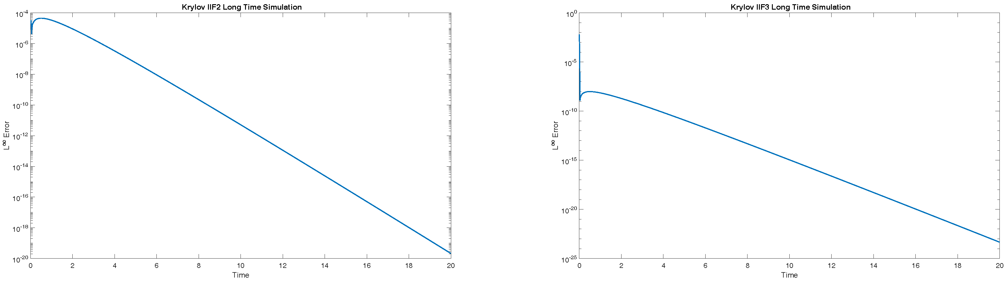
12)). From our numerical experiments in this paper, we can see that our numerical schemes have already given a clear accuracy order with very small sizes
, and
M does
not need to be increased when the spatial–temporal resolution is refined. Specifically, the second-order Krylov IIF scheme has the following form:
where
,
and
are the orthonormal basis and upper Hessenberg matrix generated by the Arnoldi algorithm with the initial vector
;
,
and
are the orthonormal basis and upper Hessenberg matrix generated by the Arnoldi algorithm with the initial vector
. The third-order Krylov IIF scheme has the following form:
where
,
and
are the orthonormal basis and upper Hessenberg matrix generated by the Arnoldi algorithm with the initial vector
;
,
and
are the orthonormal basis and upper Hessenberg matrix generated by the Arnoldi algorithm with the initial vector
;
,
and
are the orthonormal basis and upper Hessenberg matrix generated by the Arnoldi algorithm with the initial vector
. See Equation (
16) for values of
and
.
As is pointed out in [
32], in the implementation of the methods, we do
not store matrices
C, because only multiplications of matrices
C with vectors are needed in the methods, and they correspond to certain finite difference operations. In the Krylov IIF schemes (Equations (
19)–(
21)) for fourth-order PDEs, the “local implicit” property of the original IIF schemes in [
20] is preserved well; namely, the implicit terms are free of the exponential operation. As a result, the implicit nonlinear system is decoupled for each spatial grid point. The size of the implicit nonlinear system at every spatial grid point only depends on the number of original PDEs. This “local implicit” property provides a key factor for the efficiency of our high-order Krylov IIF schemes. The small-size implicit nonlinear system can be either solved analytically or efficiently solved numerically by a fixed-point iteration method [
20] or a Newton iteration method [
26].


