Cost Effectiveness Analysis of Optimal Malaria Control Strategies in Kenya

Abstract

Malaria remains a leading cause of mortality and morbidity among the children under five and pregnant women in sub-Saharan Africa, but it is preventable and controllable provided current recommended interventions are properly implemented. Better utilization of malaria intervention strategies will ensure the gain for the value for money and producing health improvements in the most cost effective way. The purpose of the value for money drive is to develop a better understanding (and better articulation) of costs and results so that more informed, evidence-based choices could be made. Cost effectiveness analysis is carried out to inform decision makers on how to determine where to allocate resources for malaria interventions. This study carries out cost effective analysis of one or all possible combinations of the optimal malaria control strategies (Insecticide Treated Bednets—ITNs, Treatment, Indoor Residual Spray—IRS and Intermittent Preventive Treatment for Pregnant Women—IPTp) for the four different transmission settings in order to assess the extent to which the intervention strategies are beneficial and cost effective. For the four different transmission settings in Kenya the optimal solution for the 15 strategies and their associated effectiveness are computed. Cost-effective analysis using Incremental Cost Effectiveness Ratio (ICER) was done after ranking the strategies in order of the increasing effectiveness (total infections averted). The findings shows that for the endemic regions the combination of ITNs, IRS, and IPTp was the most cost-effective of all the combined strategies developed in this study for malaria disease control and prevention; for the epidemic prone areas is the combination of the treatment and IRS; for seasonal areas is the use of ITNs plus treatment; and for the low risk areas is the use of treatment only. Malaria transmission in Kenya can be minimized through tailor-made intervention strategies for malaria control which produces health improvements in the most cost effective way for different epidemiological zones. This offers the good value for money for the public health programs and can guide in the allocation of malaria control resources for the post-2015 malaria eradication strategies and the achievement of the Sustainable Development Goals.

1. Introduction

Malaria is a leading cause of mortality and morbidity among the under-five and the pregnant women in Sub Saharan Africa [1]. These groups are at high risk due to weakened and immature immunity respectively. The need for value of money calls for the cost effective analysis of malaria interventions. This will also contribute to effective ways of controlling the spread of malaria in Kenya. Malaria transmission is highly variable across Kenya because of the different transmission intensities driven by climate and temperature. Kenya has four malaria epidemiological zones; the endemic areas, the seasonal malaria transmission, the malaria epidemic prone areas and the low risk malaria areas [2,3].

The current reduction in the number of malaria related cases are due to the scale up efforts of the current malaria interventions in Kenya namely use of long-lasting insecticide-treated bed nets (LLINs), indoor residual spraying (IRS), chemoprevention for most vulnerable such as intermittent preventive treatment for pregnant women (IPTp), confirmation of malaria diagnostics through rapid diagnostics tests (RDTs) and microscopy for every suspected case (case management) and timely treatment with artemisinin-based combination therapies (ACTs) [1,3]. As scale up effort increases, it is important to understand how these interventions can be optimally allocated alongside one another and on a large scale for different transmission settings. In addition, there are few guidelines about how best to deploy scarce resources for malaria control.

Cost effectiveness analysis has become an important tool in understanding the dynamics of disease transmission and in decision making processes regarding intervention programs for disease control [4,5]. Cost effectiveness analysis is carried out to inform decision makers on how to determine where to allocate resources for malaria interventions especially when they are limited. The analysis compares the costs and health effects of an intervention to assess the extent to which it can be regarded as providing value for money and the choice of the technique depends on the nature of the benefits specified. Cost-effectiveness analysis is often used in the field of health services, where it may be inappropriate to monetize health effect. The most commonly used outcome measure is quality-adjusted life years (QALY) [6].

The incremental cost-effectiveness ratio (ICER) has become the common measure for cost effectiveness analysis and is calculated in order to achieve the goal of comparing the costs and the effectiveness of the intervention strategies. Ridrogues et al. [7] conducted cost effective analysis using ICER but for TB. Okosun et al. [8] conducted cost effective analysis using ICER for three malaria intervention strategies and not for different transmission settings. He further did not consider the cost effective intervention strategies for the at risk group i.e., the pregnant and the under five children. Stukey et al. [5] modeled the cost effectiveness of malaria control interventions in the highlands of western Kenya using simulation modeling in OpenMalaria modeling platform but did not consider the effect of IPTp and those at risk population. White et al. [4] conducted a systematic review costs and cost-effectiveness of malaria control interventions but not for different transmission setting and for the at risk groups. Hansena et al. [9] conducted cost effectiveness analysis of three health interventions for the pregnant women but for low transmission settings. There is no cost effectiveness analysis done for the optimal control strategies for different malaria transmission settings in Kenya considering the at risks age groups.

IPTp is one of the WHO recommended prevention therapy for the pregnant women. IPTp has been shown to be effective in reducing maternal and infant mortality that are related to malaria for the most at risk group for malaria [10,11,12,13]. No cost effectiveness analysis has been done for the IPTp. In this study, we carry out cost effective analysis of one or all possible combinations of malaria control strategies for different transmission settings.

2. Model Formulation

The ordinary differential equations that describe the interactions between the human and mosquito population is formulated and described by Otieno et al. [14]. A deterministic malaria transmission dynamics model with intervention strategies for the most at risk groups for malaria (under five children and the pregnant women) is formulated and analyzed to investigate the optimal malaria control strategies on the transmission dynamics among the pregnant women and children under five years of age.

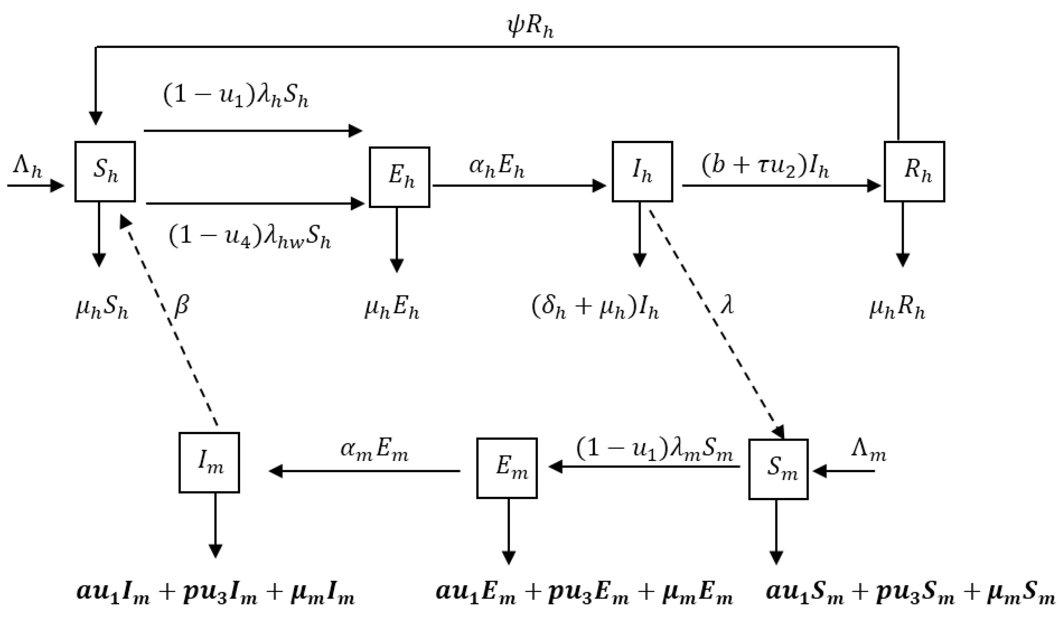
The population under study is subdivided into compartments according to the individual’s disease status. We consider a seven-dimensional model, which consists of population of Susceptible $S_h$, Exposed humans $E_h$, Infected humans $I_h$, Recovered humans $R_h$, Susceptible mosquitoes $S_m$, Exposed mosquitoes $E_m$ and Infected mosquitoes $I_m$. The total population sizes at time $t$ for humans and mosquitoes are denoted by $N_h\left(t\right)$ and $N_m\left(t\right)$ respectively. We employ the SEIRS type model for humans to describe a disease with temporary immunity on recovery from infection. Mosquitoes are assumed not to recover from the parasites so the mosquito population can be described by the SEI model. In the model we incorporate four time dependent control measures simultaneously: (i) the use of treated bednets $u_1\left(t\right)$; (ii) treatment of infective humans $u_2\left(t\right)$; (iii) spray of insecticides $u_3\left(t\right)$ and (iv) treatment to protect pregnant women and their new born children: intermittent preventive treatment (IPTp) for pregnant women $u_4\left(t\right)$. $S_h\left(t\right)$ represents the number of individuals not yet infected with the malaria parasite at time $t$, $E_h\left(t\right)$ represents individuals who are infected but not yet infectious, $I_h\left(t\right)$ is the class representing infected with malaria and are capable of transmitting the disease to susceptible mosquitoes and $R_h\left(t\right)$ represents the class of individuals who have temporarily recovered from the disease.

Figure 1 describes the dynamics of malaria in human and mosquito populations together with interventions.

The susceptible pregnant and under five humans ($S_h$) are recruited at the rate, ${\mathsf{\Lambda }}_h$. They either die from natural causes (at a rate ${\mu }_h$) or move to the exposed class ($E_h$) by acquiring malaria through contact with infectious mosquitoes at a rate $\left(1-u_1\right)\frac{\beta ϵ\varphi I_m}{N_h}{S}_h$ or $\left(1-u_4\right)\frac{\beta ϵ\varphi I_m}{N_{hw}}{S}_h$, where $\beta$ is the transmission probability per bite, $ϵ$ is the per capita biting rate of mosquitoes, $\varphi$ is the contact rate of vector per human per unit time, $u_1\left(t\right)\in \left[0,1\right]$ is the preventive measure using ITNs, $u_4\left(t\right)\in \left[0,1\right]$ is the preventive measure using IPTp, $I_m\left(t\right)$ is the infectious mosquitoes at time $t$, $N_h\left(t\right)$ is the total number of individuals (pregnant and under 5) and $N_{hw}\left(t\right)$ is the total number of pregnant women. Susceptible class $S_h$ is divided into whole population (under five years and pregnant women) being exposed and the population for the pregnant women being exposed. Exposed individuals move to the infectious class after the development of clinical symptoms at the rate ${\alpha }_h$. Infectious individuals are assumed to recover at a rate $b+\tau u_2$, where $b$ is the rate of spontaneous recovery, $u_2\left(t\right)\in \left[0,1\right]$ is the control on treatment of infected individuals and $\tau \in \left[0,1\right]$ is the efficacy of treatment. Infectious individuals who do not recover die at a rate ${\delta }_h+{\mu }_h$. Individuals infected with malaria suffer a disease induced death at rate of ${\delta }_h$, and natural death ${\mu }_h$. Infected individuals then progress to partially immune group where upon recovery the partially immune individual losses immunity at the rate $\psi$ and becomes susceptible again.

Susceptible mosquitoes ($S_m$) are recruited at the rate ${\mathsf{\Lambda }}_m$ and acquire malaria infection (following contact with humans infected with malaria) at the rate ${\lambda }_m$. They either die from natural causes (at a rate ${\mu }_m$) or move to the exposed class by acquiring malaria through contacts with infected humans at a rate $\left(1-u_1\right)\frac{\lambda ϵ\varphi I_h}{N_h}{S}_m$, where $\lambda$ is the probability for a vector to get infected after biting an infectious human and $I_h\left(t\right)$ are individuals infected by malaria at time $t$. The mosquito population is reduced, due to the use of insecticides spray, at a rate $p{u}_3$, where $u_3\left(t\right)\in \left[0,1\right]$ represents the control due to IRS and $p$ represents the efficacy of IRS. Mosquito population is also reduced as a result of natural death (${\mu }_m$) and at the rate $a{u}_1$, where $u_1\left(t\right)$ represents the control due to ITNs and $a$ is the efficacy due to ITNs. Newly infected mosquitoes are moved into the exposed class ($E_m$) at a rate ${\alpha }_m$ and progresses to the class of symptomatic mosquitoes ($I_m$).

The model is extended to formulate the optimal control problem from where cost effectiveness analysis of the optimal control strategies will be done. Following Otieno et al. [14] the state variables of the model are represented and described in

Table 1. State variables of the basic malaria model.

Symbol	Description
$S_h\left(t\right)$	Number of susceptible individuals (pregnant and under 5) at time t
$E_h\left(t\right)$	Number of exposed individuals (pregnant and under 5) at time t
$I_h\left(t\right)$	Number of infectious humans (pregnant and under 5) at time t
$R_h\left(t\right)$	Number of recovered humans (pregnant and under 5) at time t
$S_m\left(t\right)$	Number of susceptible mosquitoes at time t
$E_m\left(t\right)$	Number of exposed mosquitoes at time t
$I_m\left(t\right)$	Number of infectious mosquitoes at time t
$N_h\left(t\right)$	Total number of individuals (pregnant and under 5) at time t
$N_{hw}\left(t\right)$	Total number of pregnant individuals at time t
$N_m\left(t\right)$	Total mosquito population at time t

.

Table 2. Description of parameter variables of the malaria model.

Parameter	Description
$\varphi$	Mosquito contact rate with human
$ϵ$	Mosquito biting rate
$\beta$	Probability of human getting infected (the probability of transmission of infection from an infectious mosquito to a susceptible human provided there is a bite)
$\lambda$	Probability of a mosquito getting infected (the probability of transmission of infection from an infectious human to a susceptible mosquito provided there is a bite)
${\mu }_h$	Per capita natural death rate of humans
${\mu }_m$	Per capita natural death rate of mosquitoes
$\psi$	Per capita rate of loss of immunity by recovered individuals
${\alpha }_h$	Humans progression rate from exposed to infected
${\alpha }_m$	Mosquitoes progression rate from exposed to infected
${\mathsf{\Lambda }}_h$	Recruitment rate of human by birth and by getting pregnant
${\mathsf{\Lambda }}_m$	Recruitment of mosquitoes by birth
${\delta }_h$	Per capita disease induced death rate for humans (pregnant and under 5)
$b$	Proportion of spontaneous individual recovery
${\lambda }_h$	Force of infection for susceptible humans (pregnant and under 5) to exposed individuals
${\lambda }_{hw}$	Force of infection for susceptible pregnant humans to exposed individuals
${\lambda }_m$	Force of infection for susceptible mosquitoes to exposed mosquitoes

describes and shows parameters of the model.

Table 3. Prevention and control variables in the model.

Symbol	Description
$u_1\left(t\right)$	Preventive measure using insecticide treated bed nets (ITNs)
$u_2\left(t\right)$	The control effort on treatment of infectious individuals
$u_3\left(t\right)$	Preventing measure using indoor residual spraying (IRS)
$u_4\left(t\right)$	Preventive measure using intermittent preventive treatment for pregnant women (IPTp)
$p$	Rate constant due to use of indoor residual spraying
$\tau$	Rate constant due to use of treatment effort
$a$	Rate constant due to use of insecticide treated bed nets

describes and represents malaria prevention and control strategies practiced in Kenya.

Other assumptions of the model:

• Population for human and mosquito is constant (no immigrants)
• No recovery for infected mosquitoes
• Mosquitoes do not die to disease infection
• All parameters in the model are non-negative

Putting the above formulations and assumptions together as described by Otieno et al. [14] gives the following system of non-linear differential equations describing the dynamics of malaria in human and mosquito populations together with interventions.

The malaria dynamics model with intervention strategies being practiced in four different transmission settings in Kenya as described by Otieno et al. [14] gives the following system of differential equations

$$\begin{array}{c}\frac{d{S}_h}{dt}={\mathsf{\Lambda }}_h+\psi R_h-\left(1-u_1\right){\lambda }_h{S}_h-\left(1-u_4\right){\lambda }_{hw}{S}_h-{\mu }_h{S}_h\\ \frac{d{E}_h}{dt}=\left(1-u_1\right){\lambda }_h{S}_h+\left(1-u_4\right){\lambda }_{hw}{S}_h-\left({\alpha }_h+{\mu }_h\right)E_h\\ \frac{d{I}_h}{dt}={\alpha }_h{E}_h-\left({\delta }_h+{\mu }_h\right)I_h-\left(b+\tau u_2\right)I_h\\ \frac{d{R}_h}{dt}=\left(b+\tau u_2\right)I_h-\left(\psi +{\mu }_h\right)R_h\\ \frac{d{S}_m}{dt}={\mathsf{\Lambda }}_m-\left(1-u_1\right){\lambda }_m{S}_m-\left({\mu }_m+a{u}_1+p{u}_3\right)S_m\\ \frac{d{E}_m}{dt}=\left(1-u_1\right){\lambda }_m{S}_m-{\alpha }_m{E}_m-\left({\mu }_m+a{u}_1+p{u}_3\right)E_m\\ \frac{d{I}_m}{dt}={\alpha }_m{E}_m-\left({\mu }_m+a{u}_1+p{u}_3\right)I_m\end{array}$$

(1)

with initial conditions:

$$S_h\left(0\right)\ge 0,E_h\left(0\right)\ge 0,I_h\left(0\right)\ge 0,R_h\left(0\right)\ge 0,S_m\left(0\right)\ge 0,E_m\left(0\right)\ge 0,I_m\left(0\right)\ge 0$$

${\lambda }_m=\frac{\lambda ϵ\varphi I_h}{N_h}$ is the percapita incidence rate among mosquitoes (force of infection for susceptible mosquitoes), and ${\lambda }_h=\frac{\beta ϵ\varphi I_m}{N_h}$ is the force of infection for susceptible humans (pregnant and under 5), ${\lambda }_{hw}=\frac{\beta ϵ\varphi I_m}{N_{hw}}$ is the force of infection for susceptible pregnant humans.

The total population sizes are for the human is $N_h=S_h+E_h+I_h+R_h$ and for mosquito is $N_m=S_m+E_m+I_m$ and their differential equations are given by $\frac{d{N}_h}{dt}={\mathsf{\Lambda }}_h-{\mu }_h{N}_h-{\delta }_h{I}_h$ and $\frac{d{N}_m}{dt}={\mathsf{\Lambda }}_m-\left({\mu }_m+a{u}_1+p{u}_3\right)N_m$ respectively.

Mathematical Analysis of the Malaria Model with Intervention Strategies

The basic properties and analysis of the formulated malaria model with control strategies through mathematical analysis of the model is described and done by Otieno et al. [14].

The feasible solutions set for the Model (1) given by

$$D=\left\{\left(S_h,E_h,I_h,R_h,S_m,E_m,I_m\right)\in R_{+}^7:\left(S_h,S_m\right)>0,\left(E_h,I_h,R_h,E_m,I_m\right)\ge 0;N_h\le \frac{{\mathsf{\Lambda }}_h}{{\mu }_h};N_m\le \frac{{\mathsf{\Lambda }}_m}{{\mu }_m+a{u}_1+p{u}_3}\right\}$$

is positively-invariant and the hence Model (1) is biologically, epidemiologically meaningful and mathematically well-posed in the domain $D$.

Following Otieno et al. [14], System (1) has always a disease free equilibrium given by

$$E_0=\left(S_h^{*},E_h^{*},I_h^{*},R_h^{*},S_m^{*},E_m^{*},I_m^{*}\right)=\left(\frac{{\mathsf{\Lambda }}_h}{{\mu }_h},0,0,0,\frac{{\mathsf{\Lambda }}_m}{\left({\mu }_m+a{u}_1+p{u}_3\right)},0,0\right)$$

(2)

Basic Reproduction Number

The matrices $F$ and $V$ for the new infection terms and the remaining transfer terms at disease free equilibrium [15], respectively, are given by

$$F=\left[\begin{array}{cccc}\begin{array}{c}0\\ 0\\ 0\\ 0\end{array}& \begin{array}{c}0\\ 0\\ \frac{\left(1-u_1\right)\lambda ϵ\varphi {\mu }_h{\mathsf{\Lambda }}_m}{{\alpha }_h\left({\mu }_m+a{u}_1+p{u}_3\right)}\\ 0\end{array}& \begin{array}{c}0\\ 0\\ 0\\ 0\end{array}& \begin{array}{c}\left(1-u_1\right)\beta ϵ\varphi +\left(1-u_4\right)\beta ϵ\varphi \\ 0\\ 0\\ 0\end{array}\end{array}\right]$$

and

$$V=\left[\begin{array}{cccc}\begin{array}{c}\left({\mu }_h+{\alpha }_h\right)\\ -{\alpha }_h\\ 0\\ 0\end{array}& \begin{array}{c}0\\ \left({\delta }_h+{\mu }_h+b+\tau u_2\right)\\ 0\\ 0\end{array}& \begin{array}{c}0\\ 0\\ {\alpha }_m+{\mu }_m+a{u}_1+p{u}_3\\ -{\alpha }_m\end{array}& \begin{array}{c}0\\ 0\\ 0\\ {\mu }_m+a{u}_1+p{u}_3\end{array}\end{array}\right]$$

Following Otieno et al. [14], it follows that the basic reproduction of Model (1), denoted by $R_0$, is given by

$$R_0=\rho \left(F{V}^{-1}\right)$$

$$R_0=\sqrt{\frac{{\alpha }_h\left(1-u_1\right)\lambda ϵ\varphi {\mathsf{\Lambda }}_m{\mu }_h\left(1-u_1\right)\beta ϵ\varphi {\alpha }_m+{\alpha }_h\left(1-u_1\right)\lambda ϵ\varphi {\mathsf{\Lambda }}_m{\mu }_h\left(1-u_4\right)\beta ϵ\varphi {\alpha }_m}{\left({\mu }_m+a{u}_1+p{u}_3\right)\left({\mu }_h+{\alpha }_h\right)\left({\delta }_h+{\mu }_h+b+\tau u_2\right){\mathsf{\Lambda }}_h\left({\alpha }_m+{\mu }_m+a{u}_1+p{u}_3\right)\left({\mu }_m+a{u}_1+p{u}_3\right)}}$$

(3)

Stability Analysis of Disease Free Equilibrium Point

Local Stability of Disease Free Equilibrium Point

Theorem 1. 

The disease free equilibrium point for System (1) is locally asymptotically stable if $R_0<1$ and unstable if $R_0>1$.

Proof. 

Following Otieno et al. [14], the Jacobian matrix $\left(J\right)$ of the malaria Model (1) at the disease-free equilibrium point is given by

$$\left[\begin{array}{ccccc}\begin{array}{c}-\left({\alpha }_h+{\mu }_h\right)\\ {\alpha }_h\\ 0\\ 0\\ 0\end{array}& \begin{array}{c}0\\ -\left({\delta }_h+{\mu }_h+b+\tau u_2\right)\\ \left(b+\tau u_2\right)\\ \frac{\left(1-u_1\right)\lambda ϵ\varphi {\mathsf{\Lambda }}_m{\mu }_h}{\left({\mu }_m+a{u}_1+p{u}_3\right){\mathsf{\Lambda }}_h}\\ 0\end{array}& \begin{array}{c}0\\ 0\\ -\left(\psi +{\mu }_h\right)\\ 0\\ 0\end{array}& \begin{array}{c}0\\ 0\\ 0\\ -\left({\alpha }_m+{\mu }_m+a{u}_1+p{u}_3\right)\\ {\alpha }_m\end{array}& \begin{array}{c}\left(1-u_1\right)\beta ϵ\varphi +\left(1-u_4\right)\beta ϵ\varphi \\ 0\\ 0\\ 0\\ -\left({\mu }_m+a{u}_1+p{u}_3\right)\end{array}\end{array}\right]$$

The eigenvalues of the Jacobian matrix are the solutions of the characteristic equation

$$\left|J-\lambda I\right|=0$$

$$\left[\begin{array}{ccccc}\begin{array}{c}-\left({\alpha }_h+{\mu }_h+\lambda \right)\\ {\alpha }_h\\ 0\\ 0\\ 0\end{array}& \begin{array}{c}0\\ -\left({\delta }_h+{\mu }_h+b+\tau u_2+\lambda \right)\\ \left(b+\tau u_2\right)\\ \frac{\left(1-u_1\right)\lambda ϵ\varphi {\mathsf{\Lambda }}_m{\mu }_h}{\left({\mu }_m+a{u}_1+p{u}_3\right){\mathsf{\Lambda }}_h}\\ 0\end{array}& \begin{array}{c}0\\ 0\\ -\left(\psi +{\mu }_h+\lambda \right)\\ 0\\ 0\end{array}& \begin{array}{c}0\\ 0\\ 0\\ -\left({\alpha }_m+{\mu }_m+a{u}_1+p{u}_3+\lambda \right)\\ {\alpha }_m\end{array}& \begin{array}{c}\left(1-u_1\right)\beta ϵ\varphi +\left(1-u_4\right)\beta ϵ\varphi \\ 0\\ 0\\ 0\\ -\left({\mu }_m+a{u}_1+p{u}_3+\lambda \right)\end{array}\end{array}\right]=0$$

Expanding the determinant into a characteristic equation we have

$$-\left({\delta }_h+{\mu }_h\right)\left({\alpha }_h+{\mu }_h+\lambda \right)\left({\delta }_h+{\mu }_h+b+\tau u_2+\lambda \right)\left({\alpha }_m+{\mu }_m+a{u}_1+p{u}_3+\lambda \right)\left({\mu }_m+a{u}_1+p{u}_3+\lambda \right)-\frac{{\left(1-u_1\right)}^2\lambda {ϵ}^2{\varphi }^2{\mathsf{\Lambda }}_m{\mu }_h{\alpha }_m\beta {\alpha }_h+\left(1-u_4\right)\left(1-u_1\right)\lambda {ϵ}^2{\varphi }^2{\mathsf{\Lambda }}_m{\mu }_h{\alpha }_m\beta {\alpha }_h}{\left({\mu }_m+a{u}_1+p{u}_3\right){\mathsf{\Lambda }}_m}=0$$

(4)

Hence we have

$$A_1=\left({\mu }_m+a{u}_1+p{u}_3\right),A_2=\left({\alpha }_m+{\mu }_m+a{u}_1+p{u}_3\right),A_3=\left({\delta }_h+{\mu }_h+b+\tau u_2\right),A_4=\left({\alpha }_h+{\mu }_h\right)$$

and

$$Q=\frac{{\left(1-u_1\right)}^2\lambda {ϵ}^2{\varphi }^2{\mathsf{\Lambda }}_m{\mu }_h{\alpha }_m\beta {\alpha }_h+\left(1-u_4\right)\left(1-u_1\right)\lambda {ϵ}^2{\varphi }^2{\mathsf{\Lambda }}_m{\mu }_h{\alpha }_m\beta {\alpha }_h}{\left({\mu }_m+a{u}_1+p{u}_3\right){\mathsf{\Lambda }}_m}$$

$$\begin{array}{c}\left(\lambda +A_1\right)\left(\lambda +A_2\right)\left(\lambda +A_3\right)\left(\lambda +A_4\right)-Q=0\\ {\lambda }^4+B_1{\lambda }^3+B_2{\lambda }^2+B_3\lambda +B_4=0\end{array}$$

(5)

where

$$\begin{array}{c}{B}_1=A_4+A_3+A_2+A_1\\ B_2=A_4\left(A_3+A_2+A_1\right)+A_3\left(A_2+A_1\right)+A_1{A}_2\\ B_3=A_4{A}_3{A}_2+A_4{A}_3{A}_1+A_4{A}_2{A}_1+A_3{A}_2{A}_1\\ B_4=A_4{A}_3{A}_2{A}_1-Q\end{array}$$

(6)

Thus, applying to the Routh-Hurwitz criteria [16] to the Polynomial Equation (5), we have that all determinants of the Hurwitz matrices are positive. Hence all the eigenvalues of the Jacobian have negative real part, implying that the DFE point is stable $\left(R_0<1\right)$.

Conversely, if $R_0>1$ it implies that $B_4<0$, and since the remaining coefficients ($B_1,B_2\text{ and }{B}_3$) of the polynomial are positive then all the roots of this polynomial cannot have negative real parts. Hence, the DFE point is unstable ($R_0>1$).

Sensitivity Analysis

Sensitivity analysis to assess the relative impact of each of parameters of the basic reproductive number was done and described by Otieno et al. [14]. The normalized forward sensitivity index of the reproduction number with respect to these parameters given in

Table 4. Sensitivity indices (𝑆𝐼S) of R₀ to parameters for the malaria model.

Parameter	Sensitivity Indices
	Endemic	Seasonal	Epidemic	Low risk
${\mu }_h$	$-0.0402531$	$-0.0402531$	$-0.0402531$	$-0.0402531$
${\mu }_m$	$-1.07211$	$-1.07211$	$-1.07211$	$-1.07211$
${\alpha }_h$	$0.00038817$	$0.00038817$	$0.00038817$	$0.00038817$
${\alpha }_m$	$0.22445$	$0.22445$	$0.22445$	$0.22445$
$\lambda$	$0.5$	$0.5$	$0.5$	$0.5$
$\beta$	$0.5$	$0.5$	$0.5$	$0.5$
$ϵ$	$1$	$1$	$1$	$1$
${\mathsf{\Lambda }}_h$	$-0.4987$	$-0.4987$	$-0.4987$	$-0.4987$
${\mathsf{\Lambda }}_m$	$0.5$	$0.5$	$0.5$	$0.5$
$b$	$-0.01818$	$-0.02048$	$-0.01639$	$-0.02563$
$\tau$	$-0.322497$	$-0.322497$	$-0.322497$	$-0.322497$
${\delta }_h$	$-0.13695$	$-0.10336$	$-011321$	$-0.03508$
$\varphi$	$1$	$1$	$1$	$1$

is computed. The index measures the relative change in a variable with respect to relative changes in parameters.

Definition. 

Following Chitnis et al. [17], the normalized forward sensitivity index of a variable, $h$, that depends on a parameter, $l$, is defined as: ${\xi }_l=\frac{l}{h}\times \frac{\partial h}{\partial l}$.

Following Otieno et al. [14], the sensitivity index of the model parameters are given by

$${\xi }_{{\alpha }_h}^{R_0}=\frac{{\mu }_h}{2\left({\alpha }_h+{\mu }_h\right)}$$

$${\xi }_{{\alpha }_m}^{R_0}=\frac{p{u}_3+{\mu }_m+a{u}_1}{2\left({\alpha }_m+p{u}_3+a{u}_1+{\mu }_m\right)}$$

$${\xi }_{{\mu }_m}^{R_0}=\frac{-{\mu }_m\left(2{\alpha }_m+3\left({\mu }_m+a{u}_1+p{u}_3\right)\right)}{2\left({\alpha }_m+{\mu }_m+a{u}_1+p{u}_3\right)\left({\mu }_m+a{u}_1+p{u}_3\right)}$$

$${\xi }_{{\delta }_h}^{R_0}=\frac{-{\delta }_h}{2\left(b+\tau u_2+{\delta }_h+{\mu }_h\right)}$$

$${\xi }_b^{R_0}=\frac{-b}{2\left(b+\tau u_2+{\delta }_h+{\mu }_h\right)}$$

$${\xi }_{{\mu }_h}^{R_0}=\frac{-{\mu }_h^2+{\alpha }_h{\delta }_h+{\alpha }_{h}b+{\alpha }_h\tau u_2}{2\left({\mu }_h+{\delta }_h+b+\tau u_2\right)\left({\mu }_h+{\alpha }_h\right)}$$

Sensitivity indices for the control parameters are given by

$${\xi }_{u_1}^{R_0}=\frac{-{\mu }_1}{1-{\mu }_1}$$

$${\xi }_{u_2}^{R_0}=\frac{-\tau {\mu }_2}{2\left({\mu }_h+ϵ+b+\tau {\mu }_2\right)}$$

$${\xi }_{u_3}^{R_0}=\frac{-p\left(3p{u}_3+3{\mu }_m+a{u}_1+2{\alpha }_m\right)u_3}{2\left(p{u}_3+a{u}_1+{\mu }_m\right)\left(p{u}_3+{\mu }_m+{\alpha }_m\right)}$$

$${\xi }_{u_4}^{R_0}=\frac{-u_4}{\left(1-u_4\right)}$$

Sensitivity indices are calculated using parameters in

Table 5. Parameter values.

Parameter	Estimated Value				Source
	Endemic	Epidemic	Seasonal	Low Risk
${\mu }_h$	$0.00005447$	$0.00004644$	$0.00004281$	$0.00004566$	KNBS (2009 Census estimates) [26]
${\mu }_m$	$0.04$				Estimated
${\alpha }_h$	$0.07143$				Estimated
${\alpha }_m$	$0.0909$				Chitnis [17]
$\lambda$	$0.42$				Estimated
$\beta$	$0.0655$				Estimated
$ϵ$	$0.2$				Kbenesh et al. [27]
$\psi$	$0.01095$				Estimated
${\mathsf{\Lambda }}_h$	$0.00000575$	$0.00000575$	$0.00000548$	$0.00000438$	KNBS (estimates based on 2009 Census) [26]
${\mathsf{\Lambda }}_m$	$0.071$				Niger and Gumel [28]
$b$	$0.005$				Chiyaka et al. [29]
$\tau$	$0.5$				Assumed
${\delta }_h$	$0.05$.				KNBS and ICF Macro [30]
$p$.	$0.25$				Assumed
$a$	$0.25$				Assumed
$\varphi$	$0.502$				Kbenesh et al. [27]
${\lambda }_h$	$0.00000149$	$0.00000123$	$0.00000445$	$0.00000226$	Estimated
${\lambda }_{hw}$	$0.00000247$	$0.00000203$	$0.00000693$	$0.00000328$	Estimated
${\lambda }_m$	$0.00000048$	$0.00000394$	$0.00000143$	$0.00000073$	Estimated
$N_h$	$440169$	$535093$	$147832$	$290703$	KNBS (2009 Census estimate) [26]
$N_{hw}$	$266343$	$324658$	$94857$	$200216$	KNBS (2009 Census estimate) [26]
$N_m$	$4401690$	$5350930$	$1478320$	$2907030$	Estimated
$b_1$	$\$2.5–5.0$				White et al. [4] and Hansen et al. [9]
$b_2$	$\$2.0$				White et al. [4]
$b_3$	$\$1.50$				White et al. [4]
$b_4$	$\$2.5$				White et al. [4] and Hansen et al. [9]
$\phi$	$\raisebox{1ex}{$3$}\!\left/ \!\raisebox{-1ex}{$365$}\right.–\raisebox{1ex}{$5$}\!\left/ \!\raisebox{-1ex}{$365$}\right.\%$				Assumed

.

Through sensitivity analysis as shown by Otieno et al. [14], it is observed that the most sensitive parameters to $R_0$ across all the settings was the mosquito’s natural death rate, ${\mu }_m$, and mosquito biting rate, $ϵ$,this was followed by the by the mosquito contact rate with humans, $\varphi$, probability of mosquito getting infected, $\lambda$, the probability of humans getting infected, $\beta$, and the recruitment rate of mosquitoes and humans (see Table 4). In the next section, we start by performing an economic evaluation of the intervention strategies then use optimal control to study the optimality of these interventions. Cost-effectiveness analysis of the optimal malaria control strategies is done to determine the most cost-effective as one or combination of the four intervention strategies namely, treatment effort of infected individuals, ITNs, IRS and IPTp. Cost-effectiveness analysis is undertaken using ICER in order to assess the extent to which the intervention strategies are beneficial and cost effective. The aim is to maximizing the level of benefits (health effects) relative to the level of resources available as shown by Okosun et al. [8].

3. Economic Evaluation

The economic evaluation of all four intervention techniques is evaluated in which effectiveness and cost-effectiveness of the interventions are investigated in order to minimize or eradicate malaria disease in the area under study. The following cost objective function is used [18]

$$E_c\left(u_1,u_2,u_3,u_3\right)=\underset{\left(u_1,u_2,u_3,u_4\right)\in U}{\text{min}}{{\displaystyle \int }}_0^T\left[b_1{u}_1\left(t\right)\left(S_h\left(t\right)+S_m\left(t\right)+E_m\left(t\right)+I_m\left(t\right)\right)+b_2\tau u_2\left(t\right)I_h\left(t\right)+b_{3}p{u}_3\left(t\right)\left(S_m\left(t\right)+E_m\left(t\right)+I_m\left(t\right)\right)+b_4{u}_4\left(t\right)\left(S_h\left(t\right)+E_h\left(t\right)\right)\right]e^{-\phi t}dt$$

(7)

subject to the system of differential equation (1), where $b_1$ denotes the per unit cost of ITNs ($u_1$); $b_2$ denotes the per unit cost of treating an individual with malaria ($u_2$), $b_3$ represents the per cunit area cost of IRS effort ($u_3$) and spraying houses and $b_4$ represents the use of IPTp among the pregnant women ($u_4$). The discount rate of 3%–5% has been exponentially considered with a parameter $\phi$. The Lagrangian of the cost objective function is

$$L_b=\left[b_1{u}_1\left(t\right)\left(S_h\left(t\right)+E_h\left(t\right)+S_m\left(t\right)+E_m\left(t\right)+I_m\left(t\right)\right)+b_2\tau u_2\left(t\right)I_h\left(t\right)+b_{3}p{u}_3\left(t\right)\left(S_m\left(t\right)+E_m\left(t\right)+I_m\left(t\right)\right)+b_4{u}_4\left(t\right)\left(S_h\left(t\right)+E_h\left(t\right)\right)\right]e^{-\phi t}$$

Then the Hamiltonian equation with Lagrangian, state variables and adjoint variables is

$$H_b=L_b+{\lambda }_1^{*}\frac{d{S}_h}{dt}+{\lambda }_2^{*}\frac{d{E}_h}{dt}+{\lambda }_3^{*}\frac{d{I}_h}{dt}+{\lambda }_4^{*}\frac{d{R}_h}{dt}+{\lambda }_5^{*}\frac{d{S}_m}{dt}+{\lambda }_6^{*}\frac{d{E}_m}{dt}+{\lambda }_7^{*}\frac{d{I}_m}{dt}$$

The developed corresponding Hamiltonian equation is given by:

$$\begin{array}{cc}{H}_b=[b_1{u}_1\left(t\right)& \left(S_h\left(t\right)+E_h\left(t\right)+S_m\left(t\right)+E_m\left(t\right)+I_m\left(t\right)\right)+b_2\tau u_2\left(t\right)I_h\left(t\right)\hfill \\ & +b_{3}p{u}_3\left(t\right)\left(S_m\left(t\right)+E_m\left(t\right)+I_m\left(t\right)\right)+b_4{u}_4\left(S_h\left(t\right)+E_h\left(t\right)\right)]e^{-\phi t}\hfill \\ & +\left\{{\mathsf{\Lambda }}_h+\psi R_h-\left(1-u_1\right){\lambda }_h{S}_h-\left(1-u_4\right){\lambda }_{hw}{S}_h-{\mu }_h{S}_h\right\}{\lambda }_1^{*}\hfill \\ & +\left\{\left(1-u_1\right){\lambda }_h{S}_h+\left(1-u_4\right){\lambda }_{hw}{S}_h-\left({\alpha }_h+{\mu }_h\right)E_h\right\}{\lambda }_2^{*}\hfill \\ & +\left\{{\alpha }_h{E}_h-\left({\delta }_h+{\mu }_h\right)I_h-\left(b+\tau u_2\right)I_h\right\}{\lambda }_3^{*}+\left\{\left(b+\tau u_2\right)I_h-\left(\psi +{\mu }_h\right)R_h\right\}{\lambda }_4^{*}\hfill \\ & +\left\{{\mathsf{\Lambda }}_m-\left(1-u_1\right){\lambda }_m{S}_m-\left({\mu }_m+a{u}_1+p{u}_3\right)S_m\right\}{\lambda }_5^{*}\hfill \\ & +\left\{\left(1-u_1\right){\lambda }_m{S}_m-{\alpha }_m{E}_m-\left({\mu }_m+a{u}_1+p{u}_3\right)E_m\right\}{\lambda }_6^{*}\hfill \\ & +\left\{{\alpha }_m{E}_m-\left({\mu }_m+a{u}_1+p{u}_3\right)I_m\right\}{\lambda }_7^{*}\hfill \end{array}$$

(8)

where ${\lambda }_1^{*},{\lambda }_2^{*},{\lambda }_3^{*},{\lambda }_4^{*},{\lambda }_5^{*},{\lambda }_6^{*}$ and ${\lambda }_7^{*}$ denote the marginal value/ shadow prices linked to their corresponding classes. The ${\lambda }_i^{*}$ where $i=\left(1,2,\dots ,7\right)$ represent the changes in the objective value of an optimal solution of an optimization problem by relaxing the constraint by one unit [18]. These can be calculated by using Pontryagin’s Maximum Principle:

$$\frac{d{\lambda }_1^{*}}{dt}=-\frac{\partial H_b}{\partial S_h},\frac{d{\lambda }_2^{*}}{dt}=-\frac{\partial H_b}{\partial E_h},\frac{d{\lambda }_3^{*}}{dt}=-\frac{\partial H_b}{\partial I_h},\frac{d{\lambda }_4^{*}}{dt}=-\frac{\partial H_b}{\partial R_h}$$

$$\frac{d{\lambda }_5^{*}}{dt}=-\frac{\partial H_b}{\partial S_m},\frac{d{\lambda }_6^{*}}{dt}=-\frac{\partial H_b}{\partial E_m},\frac{d{\lambda }_7^{*}}{dt}=-\frac{\partial H_b}{\partial I_m}$$

Hence using the Hamiltonian Equation (8) gives

$$\begin{array}{c}\frac{d{\lambda }_1^{*}}{dt}=-\frac{\partial H_b}{\partial S_h}=-b_1{u}_1{e}^{-\phi t}-b_4{u}_4{e}^{-\phi t}+\left(1-u_1\right)\frac{\beta ϵ\varphi I_m}{N_h}{\lambda }_1^{*}+\left(1-u_4\right)\frac{\beta ϵ\varphi I_m}{N_{hw}}{\lambda }_1^{*}+{\mu }_h{\lambda }_1^{*}-\left(1-u_1\right)\frac{\beta ϵ\varphi I_m}{N_h}{\lambda }_2^{*}-\left(1-u_4\right)\frac{\beta ϵ\varphi I_m}{N_{hw}}{\lambda }_2^{*}\\ \frac{d{\lambda }_2^{*}}{dt}=-\frac{\partial H_b}{\partial E_h}=-b_1{u}_1{e}^{-\phi t}-b_4{u}_4{e}^{-\phi t}+{\alpha }_h{\lambda }_2^{*}+{\mu }_h{\lambda }_2^{*}-{\alpha }_h{\lambda }_3^{*}\\ \frac{d{\lambda }_3^{*}}{dt}=-\frac{\partial H_b}{\partial I_h}=-b_2\tau u_2{e}^{-\phi t}+\left(b+\tau u_2+{\mu }_h+{\delta }_h\right){\lambda }_3^{*}-\left(b+\tau u_2\right){\lambda }_4^{*}+\left(\frac{\left(1-u_1\right)\lambda ϵ\varphi S_m}{N_h}\right){\lambda }_5-\left(\frac{\left(1-u_1\right)\lambda ϵ\varphi S_m}{N_h}\right){\lambda }_6\\ \frac{d{\lambda }_4^{*}}{dt}=-\frac{\partial H_b}{\partial R_h}=-\psi {\lambda }_1^{*}+\left({\mu }_h+\psi \right){\lambda }_4^{*}\\ \frac{d{\lambda }_5^{*}}{dt}=-\frac{\partial H_b}{\partial S_m}=-b_1{u}_1{e}^{-\phi t}-b_{3}p{u}_3{e}^{-\phi t}+\left(1-u_1\right)\frac{\lambda ϵ\varphi I_h}{N_h}{\lambda }_5^{*}+\left({\mu }_m+a{u}_1+p{u}_3\right){\lambda }_5^{*}-\left(1-u_1\right)\frac{\lambda ϵ\varphi I_h}{N_h}{\lambda }_6^{*}\\ \frac{d{\lambda }_6^{*}}{dt}=-\frac{\partial H_b}{\partial E_m}=-b_1{u}_1{e}^{-\phi t}-b_{3}p{u}_3{e}^{-\phi t}+\left({\alpha }_m+{\mu }_m+a{u}_1+p{u}_3\right){\lambda }_6^{*}+{\alpha }_m{\lambda }_6^{*}-{\alpha }_m{\lambda }_7^{*}\\ \frac{d{\lambda }_7^{*}}{dt}=-\frac{\partial H_b}{\partial I_m}=-b_1{u}_1{e}^{-\phi t}-b_{3}p{u}_3{e}^{-\phi t}+\left({\mu }_m+a{u}_1+p{u}_3\right){\lambda }_7^{*}+\left(\frac{\left(1-u_1\right)\beta ϵ\varphi S_h}{N_h}+\frac{\left(1-u_4\right)\beta ϵ\varphi S_h}{N_{hw}}\right){\lambda }_1+\left(-\frac{\left(1-u_1\right)\beta ϵ\varphi S_h}{N_h}-\frac{\left(1-u_4\right)\beta ϵ\varphi S_h}{N_{hw}}\right){\lambda }_2\end{array}$$

(9)

Each intervention strategy is assessed by developing the Hamiltonian equation thereafter the economic tool will be employed.

3.1. Economic Evaluation of ITNs

The prevention parameter for the ITNs is denoted by $u_1\left(t\right)$. The Hamiltonian equation, $H_b$, is differentiated with respect to $u_1$ to obtain

$$\frac{\partial H_b}{\partial u_1}=-b_1{e}^{-\phi t}\left(S_h\left(t\right)+E_h\left(t\right)+S_m\left(t\right)+E_m\left(t\right)+I_m\left(t\right)\right)+\frac{\beta ϵ\varphi I_m{S}_h}{N_h}\left({\lambda }_2^{*}-{\lambda }_1^{*}\right)+\left({\lambda }_6-{\lambda }_5\right)\frac{\lambda ϵ\varphi I_h}{N_h}{S}_m^{*}+a\left(S_m{\lambda }_5^{*}+E_m{\lambda }_6^{*}+I_m{\lambda }_7^{*}\right)$$

in which $\frac{\beta ϵ\varphi I_m{S}_h}{N_h}\left({\lambda }_1^{*}-{\lambda }_2^{*}\right)+\left({\lambda }_6-{\lambda }_5\right)\frac{\lambda ϵ\varphi I_h}{N_h}{S}_m^{*}+a\left(S_m{\lambda }_5^{*}+E_m{\lambda }_6^{*}+I_m{\lambda }_7^{*}\right)$ is the total marginal benefit due to the use of ITNs while $b_1{e}^{-\phi t}\left(S_h\left(t\right)+E_h\left(t\right)+S_m\left(t\right)+E_m\left(t\right)+I_m\left(t\right)\right)$ is the marginal cost of acquiring the ITNs. The equivalency of the marginal cost and marginal benefit leads one to achieve the optimal policy.

Hence

$$u_1\left(t\right)=\{\begin{array}{c}0if{b}_1{e}^{-\phi t}\left(S_h+E_h+S_m+E_m+I_m\right)>\frac{\beta ϵ\varphi I_m{S}_h}{N_h}\left({\lambda }_2^{*}-{\lambda }_1^{*}\right)+\left({\lambda }_6-{\lambda }_5\right)\frac{\lambda ϵ\varphi I_h}{N_h}{S}_m^{*}+a\left(S_m{\lambda }_5^{*}+E_m{\lambda }_6^{*}+I_m{\lambda }_7^{*}\right)\\ \left(0,1\right)if{b}_1{e}^{-\phi t}\left(S_h+E_h+S_m+E_m+I_m\right)=\frac{\beta ϵ\varphi I_m{S}_h}{N_h}\left({\lambda }_2^{*}-{\lambda }_1^{*}\right)+\left({\lambda }_6-{\lambda }_5\right)\frac{\lambda ϵ\varphi I_h}{N_h}{S}_m^{*}+a\left(S_m{\lambda }_5^{*}+E_m{\lambda }_6^{*}+I_m{\lambda }_7^{*}\right)\\ 1if{b}_1{e}^{-\phi t}\left(S_h+E_h+S_m+E_m+I_m\right)<\frac{\beta ϵ\varphi I_m{S}_h}{N_h}\left({\lambda }_2^{*}-{\lambda }_1^{*}\right)+\left({\lambda }_6-{\lambda }_5\right)\frac{\lambda ϵ\varphi I_h}{N_h}{S}_m^{*}+a\left(S_m{\lambda }_5^{*}+E_m{\lambda }_6^{*}+I_m{\lambda }_7^{*}\right)\end{array}$$

(10)

The third part of equation (10), shows that if this is achieved then the total marginal benefit of using ITNs is more than the total marginal cost; hence the gain of optimal malaria prevention. Then we can conclude that the susceptible and exposed individuals should best (effectively) use this prevention strategy in order to fight the epidemic. On the other hand, few susceptible and exposed individuals will use ITNs if the marginal cost is more than the marginal benefit. The effective use of this strategy will lead to achieve the optimal policy which says that increasing the use of ITNs increases the number of susceptible humans and uninfected mosquitoes.

3.2. Economic Evaluation of Treatment Effort of Infected Individuals

Here the control parameter for treatment of infectious individuals is given by $u_2\left(t\right)$. The Hamiltonian equation, $H_b$, Equation (8) is differentiated with respect to $u_2\left(t\right)$, giving

$$\frac{\partial H_b}{\partial u_1}=-b_2\tau I_h{e}^{-\phi t}+\tau I_h\left({\lambda }_4^{*}-{\lambda }_3^{*}\right)$$

in which $b_2\tau I_h$ is the marginal cost and $\tau I_h\left({\lambda }_4^{*}-{\lambda }_3^{*}\right)$ is the marginal benefit of treating infectious individuals. Hence,

$$u_2\left(t\right)=\{\begin{array}{c}0if{b}_2\tau I_h{e}^{-\phi t}>\tau I_h\left({\lambda }_4^{*}-{\lambda }_3^{*}\right)\\ \left(0,1\right)if{b}_2\tau I_h{e}^{-\phi t}=\tau I_h\left({\lambda }_4^{*}-{\lambda }_3^{*}\right)\\ 1if{b}_2\tau I_h{e}^{-\phi t}<\tau I_h\left({\lambda }_4^{*}-{\lambda }_3^{*}\right)\end{array}$$

(11)

The optimal policy is to ensure that the marginal costs for being treated is equal to the marginal benefit for the individuals being treated. Therefore, from Equation (11) all infected individuals must look for full treatment if the marginal benefit, $I_h\left({\lambda }_4^{*}-{\lambda }_3^{*}\right)$, must be greater than the marginal cost, $b_2\tau I_h{e}^{-\phi t}$, for being treated. Otherwise, only few infected individuals will look for treatment.

3.3. Economic Evaluation of IRS

Insecticide residual spraying (IRS) prevention parameter in the Hamiltonian equation, $H_b$, Equation (8) is $u_3\left(t\right)$. Then differentiating $H_b$ with respect to $u_3$ gives

$$\frac{\partial H_b}{\partial u_3}=b_{3}p\left(S_m+E_m+I_m\right)e^{-\phi t}-p\left(S_m{\lambda }_5^{*}+E_m{\lambda }_6^{*}+I_m{\lambda }_7^{*}\right)$$

where $b_{3}p\left(S_m+E_m+I_m\right)$ is the marginal cost for IRS and $p\left(S_m{\lambda }_5^{*}+E_m{\lambda }_6^{*}+I_m{\lambda }_7^{*}\right)$ is the marginal benefit for using the sprayed houses. Furthermore, it can be deduced that the optimal policy for a sprayed house is given by

$$u_3\left(t\right)=\{\begin{array}{c}0if{b}_{3}p\left(S_m+E_m+I_m\right)e^{-\phi t}>p\left(S_m{\lambda }_5^{*}+E_m{\lambda }_6^{*}+I_m{\lambda }_7^{*}\right)\\ \left(0,1\right)if{b}_{3}p\left(S_m+E_m+I_m\right)e^{-\phi t}=p\left(S_m{\lambda }_5^{*}+E_m{\lambda }_6^{*}+I_m{\lambda }_7^{*}\right)\\ 1if{b}_{3}p\left(S_m+E_m+I_m\right)e^{-\phi t}<p\left(S_m{\lambda }_5^{*}+E_m{\lambda }_6^{*}+I_m{\lambda }_7^{*}\right)\end{array}$$

(12)

The spraying of insecticides against mosquitoes is optimal for malaria disease control if the marginal cost $b_{3}p\left(S_m+E_m+I_m\right)$, is less than the marginal benefit, $p\left(S_m{\lambda }_5^{*}+E_m{\lambda }_6^{*}+I_m{\lambda }_7^{*}\right)$).

3.4. Economic Evaluation of IPTp

Intermittent Preventive Treatment (IPTp) prevention parameter in the Hamiltonian equation, $H_b$, Equation (8) is $u_4\left(t\right)$. Then differentiating $H_b$with respect to $u_4$ gives

$$\frac{\partial H_b}{\partial u_4}=-b_4{e}^{-\phi t}\left(S_h+E_h\right)+\frac{\beta ϵ\varphi I_m{S}_h}{N_{hw}}\left({\lambda }_2^{*}-{\lambda }_1^{*}\right)$$

in which $\frac{\beta ϵ\varphi I_m{S}_h}{N_{hw}}\left({\lambda }_2^{*}-{\lambda }_1^{*}\right)$ is the total marginal benefit due to the use of IPTp while $b_4{e}^{-\phi t}\left(S_h+E_h\right)$ is the marginal cost of acquiring the IPTp. The equivalency of the marginal cost and marginal benefit leads one to achieve the optimal policy.

Hence

$$u_4\left(t\right)=\{\begin{array}{c}0if{b}_4{e}^{-\phi t}\left(S_h+E_h\right)>\frac{\beta ϵ\varphi I_m{S}_h}{N_{hw}}\left({\lambda }_2^{*}-{\lambda }_1^{*}\right)\\ \left(0,1\right)if{b}_4{e}^{-\phi t}\left(S_h+E_h\right)=\frac{\beta ϵ\varphi I_m{S}_h}{N_{hw}}\left({\lambda }_2^{*}-{\lambda }_1^{*}\right)\\ 1if{b}_4{e}^{-\phi t}\left(S_h+E_h\right)<\frac{\beta ϵ\varphi I_m{S}_h}{N_{hw}}\left({\lambda }_2^{*}-{\lambda }_1^{*}\right)\end{array}$$

(13)

4. Analysis of Optimal Control

We consider the objective function

$$J\left(u_1,u_2,u_3,u_4\right)={{\displaystyle \int }}_0^T\left(A_1{N}_m+A_2{I}_h+A_3{E}_h+\left(B_1{u}_1^2+B_2{u}_2^2+B_3{u}_3^2+B_4{u}_4^2\right)\right)e^{-\phi t}dt$$

(14)

subject to

$$\frac{d{S}_h}{dt}={\mathsf{\Lambda }}_h+\psi R_h-\left(1-u_1\right){\lambda }_h{S}_h-\left(1-u_4\right){\lambda }_{hw}{S}_h-{\mu }_h{S}_h$$

$$\frac{d{E}_h}{dt}=\left(1-u_1\right){\lambda }_h{S}_h+\left(1-u_4\right){\lambda }_{hw}{S}_h-\left({\alpha }_h+{\mu }_h\right)E_h$$

$$\frac{d{I}_h}{dt}={\alpha }_h{E}_h-\left({\delta }_h+{\mu }_h\right)I_h-\left(b+\tau u_2\right)I_h$$

$$\frac{d{R}_h}{dt}=\left(b+\tau u_2\right)I_h-\left(\psi +{\mu }_h\right)R_h$$

$$\frac{d{S}_m}{dt}={\mathsf{\Lambda }}_m-\left(1-u_1\right){\lambda }_m{S}_m-\left({\mu }_m+a{u}_1+p{u}_3\right)S_m$$

$$\frac{d{E}_m}{dt}=\left(1-u_1\right){\lambda }_m{S}_m-{\alpha }_m{E}_m-\left({\mu }_m+a{u}_1+p{u}_3\right)E_m$$

$$\frac{d{I}_m}{dt}={\alpha }_m{E}_m-\left({\mu }_m+a{u}_1+p{u}_3\right)I_m$$

$$S_h\left(0\right)\ge 0,E_h\left(0\right)\ge 0,I_h\left(0\right)\ge 0,R_h\left(0\right)\ge 0,S_m\left(0\right)\ge 0,E_m\left(0\right)\ge 0,I_m\left(0\right)\ge 0$$

And the total cost at time $t$ is given by

$$C={{\displaystyle \int }}_0^T\left[b_1{u}_1\left(S_h+S_m+E_m+I_m\right)+b_2{u}_2{I}_h+b_3{u}_3\left(S_m+E_m+I_m\right)+b_4{u}_4\left(S_h+E_h\right)\right]dt$$

(15)

where $A_1,A_2,A_3,B_1,B_2,B_3,B_4$ are desired positive weights on the benefits of preventing infection and exposure plus total mosquito population. Here, we assume that there is no linear relationship between the coverage of these interventions and their corresponding costs, hence we choose a quadratic cost on the controls in keeping with what is in other literature on cost of control of epidemics [8,19,20,21]. Our goal with the given objective function is to minimize the number of infected humans, exposed humans and total mosquito population while minimizing the cost of control $u_1\left(t\right),u_2\left(t\right),u_3\left(t\right)$ and $u_4\left(t\right)$. We seek an optimal control $u_1^{*},u_2^{*},u_3^{*}$ and $u_4^{*}$ such that

$$J\left(u_1^{*},u_2^{*},u_3^{*},u_4^{*}\right)=\underset{u_1,u_2,u_3,u_4ϵU}{\text{min}}J\left(u_1,u_2,u_3,u_4\right)$$

(16)

Where $U$ is the set of measurable functions defined from $\left[0,T\right]$ onto $\left[0,1\right]$.

The necessary conditions that an optimal control must satisfy come from the Pontryagin’s Maximum Principle [18]. This consists in minimizing, with respect to $\left(u_1,u_2,u_3,u_4\right)$/

Forming the Hamiltonian from the objective function (14) subject to Equations (1) and (15)

$$\begin{array}{cc}H=(A_1{N}_m+& A_2{I}_h+A_3{E}_h+\left(B_1{u}_1^2+B_2{u}_2^2+B_3{u}_3^2+B_4{u}_4^2\right))e^{-\phi t}\hfill \\ & +\left\{{\Lambda }_h+\psi R_h-\left(1-u_1\right){\lambda }_h{S}_h-\left(1-u_4\right){\lambda }_{hw}{S}_h-{\mu }_h{S}_h\right\}{\lambda }_1\hfill \\ & +\left\{\left(1-u_1\right){\lambda }_h{S}_h+\left(1-u_4\right){\lambda }_{hw}{S}_h-\left({\alpha }_h+{\mu }_h\right)E_h\right\}{\lambda }_2\hfill \\ & +\left\{{\alpha }_h{E}_h-\left({\delta }_h+{\mu }_h\right)I_h-\left(b+\tau u_2\right)I_h\right\}{\lambda }_3+\left\{\left(b+\tau u_2\right)I_h-\left(\psi +{\mu }_h\right)R_h\right\}{\lambda }_4\hfill \\ & +\left\{{\Lambda }_m-\left(1-u_1\right){\lambda }_m{S}_m-\left({\mu }_m+a{u}_1+p{u}_3\right)S_m\right\}{\lambda }_5\hfill \\ & +\left\{\left(1-u_1\right){\lambda }_m{S}_m-{\alpha }_m{E}_m-\left({\mu }_m+a{u}_1+p{u}_3\right)E_m\right\}{\lambda }_6\hfill \\ & +\left\{{\alpha }_m{E}_m-\left({\mu }_m+a{u}_1+p{u}_3\right)I_m\right\}{\lambda }_7\hfill \\ & +\{[b_1{u}_1\left(S_h+S_m+E_m+I_m\right)+b_2{u}_2{I}_h+b_3{u}_3\left(S_m+E_m+I_m\right)\hfill \\ & +b_4{u}_4\left(S_h+E_h\right)\left]\right\}{\lambda }_C\hfill \end{array}$$

(17)

where ${\lambda }_1,{\lambda }_2,{\lambda }_3,{\lambda }_4,{\lambda }_5,{\lambda }_6$ and ${\lambda }_7$ are the adjoint variables or co-state variables given by the following system:

$$\begin{array}{c}\frac{d{\lambda }_1}{dt}=-\frac{\partial H}{\partial S_h}=\left(1-u_1\right)\frac{\beta ϵ\varphi I_m}{N_h}{\lambda }_1^{*}+\left(1-u_4\right)\frac{\beta ϵ\varphi I_m}{N_{hw}}{\lambda }_1^{*}+{\mu }_h{\lambda }_1^{*}-\left(1-u_1\right)\frac{\beta ϵ\varphi I_m}{N_h}{\lambda }_2^{*}-\left(1-u_4\right)\frac{\beta ϵ\varphi I_m}{N_{hw}}{\lambda }_2^{*}-{\lambda }_C\left(b_1{u}_1+b_4{u}_4\right)\\ \frac{d{\lambda }_2}{dt}=-\frac{\partial H}{\partial E_h}=-A_3+{\alpha }_h{\lambda }_2^{*}+{\mu }_h{\lambda }_2^{*}-{\alpha }_h{\lambda }_3^{*}-{\lambda }_C\left(b_1{u}_1+b_4{u}_4\right)\\ \frac{d{\lambda }_3}{dt}=-\frac{\partial H}{\partial I_h}=-A_2+\left(b+\tau u_2+{\mu }_h+{\delta }_h\right){\lambda }_3^{*}-\left(b+\tau u_2\right){\lambda }_4^{*}-{\lambda }_C{b}_2{u}_2+\left(\frac{\left(1-u_1\right)\lambda ϵ\varphi S_m}{N_h}\right){\lambda }_5-\left(\frac{\left(1-u_1\right)\lambda ϵ\varphi S_m}{N_h}\right){\lambda }_6\\ \frac{d{\lambda }_4}{dt}=-\frac{\partial H}{\partial R_h}=-\psi {\lambda }_1^{*}+\left({\mu }_h+\psi \right){\lambda }_4^{*}\\ \frac{d{\lambda }_5}{dt}=-\frac{\partial H}{\partial S_m}=-A_1+\left(1-u_1\right)\frac{\lambda ϵ\varphi I_h}{N_h}{\lambda }_5^{*}+\left({\mu }_m+a{u}_1+p{u}_3\right){\lambda }_5^{*}-\left(1-u_1\right)\frac{\lambda ϵ\varphi I_h}{N_h}{\lambda }_6^{*}-{\lambda }_C\left(b_1{u}_1+b_3{u}_3\right)\\ \frac{d{\lambda }_6}{dt}=-\frac{\partial H}{\partial E_m}=-A_1+{\alpha }_m{\lambda }_6^{*}+\left({\alpha }_m+{\mu }_m+a{u}_1+p{u}_3\right){\lambda }_6^{*}-{\alpha }_m{\lambda }_7^{*}-{\lambda }_C\left(b_1{u}_1+b_3{u}_3\right)\\ \frac{d{\lambda }_6}{dt}=-\frac{\partial H}{\partial E_m}=-A_1+{\alpha }_m{\lambda }_6^{*}+\left({\alpha }_m+{\mu }_m+a{u}_1+p{u}_3\right){\lambda }_6^{*}-{\alpha }_m{\lambda }_7^{*}-{\lambda }_C\left(b_1{u}_1+b_3{u}_3\right)\\ \frac{d{\lambda }_7}{dt}=-\frac{\partial H}{\partial I_m}=-A_1+({\mu }_m+a{u}_1+p{u}_3){\lambda }_7^{*}-{\lambda }_c(b_1{u}_1+b_3{u}_3)+(\frac{(1-u_1)\beta ϵ\varphi S_h}{N_h}+\frac{(1-u_4)\beta ϵ\varphi S_h}{N_{hw}}){\lambda }_1+(\frac{(1-u_1)\beta ϵ\varphi S_h}{N_h}-\frac{(1-u_4)\beta ϵ\varphi S_h}{N_{hw}}){\lambda }_2\\ \frac{d{\lambda }_C}{dt}=0\end{array}$$

(18)

By applying Pontryagin’s Maximum Principle [18] and the existence result for the optimal control from Fleming and Rishel [22], we obtain

Proposition 1. 

The optimal control $\left(u_1^{*},u_2^{*},u_3^{*},u_4^{*}\right)$ that minimizes $J\left(u_1,u_2,u_3,u_4\right)$ over $U$ is given by

$$\begin{array}{c}{u}_1^{*}=max\left\{0,min\left(1,\frac{\left({\lambda }_2-{\lambda }_1\right){\lambda }_h{S}_h^{*}+\left({\lambda }_6-{\lambda }_5\right){\lambda }_m{S}_m^{*}+a{S}_m^{*}{\lambda }_5+a{E}_m^{*}{\lambda }_6+a{I}_m^{*}{\lambda }_7+{\lambda }_C{b}_1\left(S_h^{*}+S_m^{*}\right)}{2B_1{e}^{-\phi t}}\right)\right\}\\ u_2^{*}=max\left\{0,min\left(1,\frac{\left(\tau \left({\lambda }_3-{\lambda }_4\right)I_h^{*}+{\lambda }_C{b}_2{I}_h^{*}\right)e^{\phi t}}{B_2}\right)\right\}\\ u_3^{*}=max\left\{0,min\left(1,\frac{\left(p\left({\lambda }_5{S}_m^{*}+{\lambda }_6{E}_m^{*}+{\lambda }_7{I}_m^{*}\right)+{\lambda }_C{b}_3\left(S_m^{*}+E_m^{*}+I_m^{*}\right)\right)e^{\phi t}}{B_3}\right)\right\}\\ u_4^{*}=max\left\{0,min\left(1,\frac{\left({\lambda }_2-{\lambda }_1\right){\lambda }_{hw}{S}_h^{*}+{\lambda }_C{b}_4\left(S_h^{*}+E_h^{*}\right)}{2B_4{e}^{-\phi t}}\right)\right\}\end{array}$$

(19)

where ${\lambda }_1,{\lambda }_2,{\lambda }_3,{\lambda }_4,{\lambda }_5,{\lambda }_6$ and ${\lambda }_7$ are the adjoint variables or co-state variables satisfying Equation (18) and the following transversality conditions:

$${\lambda }_1\left(T\right)={\lambda }_2\left(T\right)={\lambda }_3\left(T\right)={\lambda }_4\left(T\right)={\lambda }_5\left(T\right)={\lambda }_6\left(T\right)={\lambda }_7\left(T\right)={\lambda }_C\left(T\right)=0$$

(20)

Proof. 

From Fleming and Rishel [22], the existence of an optimal control is a consequence of the convexity of the integrand of $J$ with respect to $u_1,u_2,u_3,u_4$, a priori boundedness of the state variables, and the Lipschitz property of the state system with respect to the state variables. The differential equations governing the adjoint variables are obtained by differentiation of the Hamiltonian function, evaluated at the optimal control. Then the adjoint system can be written as,

$$0=\frac{\partial H}{\partial u_1}=-u_1^{c}2B_1{e}^{-\phi t}+\left({\lambda }_2-{\lambda }_1\right){\lambda }_h{S}_h^{*}+\left({\lambda }_6-{\lambda }_5\right){\lambda }_m{S}_m^{*}+a{S}_m^{*}{\lambda }_5+a{E}_m^{*}{\lambda }_6+a{I}_m^{*}{\lambda }_7+{\lambda }_C{b}_1\left(S_h^{*}+S_m^{*}\right)$$

$$0=\frac{\partial H}{\partial u_2}=u_2^{c}2B_2-\left(\tau \left({\lambda }_3-{\lambda }_4\right)I_h^{*}+{\lambda }_C{b}_2{I}_h^{*}\right)e^{\phi t}$$

$$0=\frac{\partial H}{\partial u_3}=u_3^{c}2B_3-\left(p\left({\lambda }_5{S}_m^{*}+{\lambda }_6{E}_m^{*}+{\lambda }_7{I}_m^{*}\right)+{\lambda }_C{b}_3\left(S_m^{*}+E_m^{*}+I_m^{*}\right)\right)e^{\phi t}$$

$$0=\frac{\partial H}{\partial u_4}=-u_4^{c}2B_4{e}^{-\phi t}-\left({\lambda }_2-{\lambda }_1\right){\lambda }_{hw}{S}_h^{*}+{\lambda }_C{b}_4\left(S_h^{*}+E_h^{*}\right)$$

Due to the a priori boundedness of the solutions of both the state and adjoint equations and the resulting Lipschitz structure of these equations, we obtain the uniqueness of the optimality Systems ((18)–(20)) for small $T$.

The restriction on the length of time interval $\left[0,T\right]$ is common in control problems [8,21,23], and it guarantees the uniqueness of the optimality system.

By standard control arguments involving the bounds on the controls, we conclude that

$$u_1^{*}=\{\begin{array}{c}0if{u}_1^c\le 0\\ u_1^{c}if0<u_1^c<1\\ 1if{u}_1^c\ge 0\end{array},u_2^{*}=\{\begin{array}{c}0if{u}_2^c\le 0\\ u_2^{c}if0<u_2^c<1\\ 1if{u}_2^c\ge 0\end{array},u_3^{*}=\{\begin{array}{c}0if{u}_3^c\le 0\\ u_1^{c}if0<u_3^c<1\\ 1if{u}_3^c\ge 0\end{array},u_4^{*}=\{\begin{array}{c}0if{u}_4^c\le 0\\ u_1^{c}if0<u_4^c<1\\ 1if{u}_4^c\ge 0\end{array}$$

Following Otieno et al. [24], the optimal control is obtained by solving the optimality Systems ((18)–(20)). An iterative scheme is used for solving the optimality system. We start by solving the state equations with a guess for the controls over the simulated time using fourth order Runge-Kutta scheme. Because of the transversality conditions (20), the adjoint equations are solved by the backward fourth order Runge-Kutta scheme using the current iterations solutions of the state equation. Then the controls are updated by using a convex combination of the previous controls and the value from the characterizations (19). This process is repeated and iterations stopped if the values of the unknowns at the previous iterations are very close to the ones at the present iterations as also described by Lenhart and Workman [25].

Parameter values from Table 5 are used for the numerical simulation

5. Cost-Effectiveness Analysis

We use a more classical approach to analyze the cost-effectiveness of the 15 alternative strategies by using the ICER in Okosun et al. [8]. ICER is applied to achieve the goal of comparing the costs and the health outcomes of two alternative intervention strategies that compete for the same resources. It is generally described as the additional cost per additional health outcomes. ICER is given by

$$ICERforQ=\frac{CostofInterventionQ-CostofInterventionP}{EffectofInterventionQ-EffectofInterventionP}$$

where $P$ and $Q$ are the two intervention strategies being compared in this case, and the effect or benefits in health status are measured in terms of quality-adjusted life years (QALYs) gained or lost. Alternatives that are more expensive and less ineffective are then excluded. This is done after simulating the optimal control model and then ranking strategies in order of increasing effectiveness measured as the total infections averted.

6. Numerical Results and Discussion

The parameters in the Model (1) were estimated using clinical malaria data and demographics statistics of Kenya. Those that were not available were obtained from literature published by researchers in malaria endemic countries which have similar environmental conditions compare to Kenya. Table 5 provides a summary of the estimated values of all parameters as described by Otieno et al. [23] in addition to some from the literature. Data was collected from the literature, Division of Malaria Control (DOMC), Kenya National Bureau of Statistics, Malaria Indicator Survey for Kenya, Demographic Health Survey (DHS) for Kenya, WHO websites and hospital records (from Kisumu, Kisii, Chuka (Tharake-Nithi) and Nyeri counties representing the four different transmission settings/epidemiological zones in Kenya).

In addition the effect of the different intervention strategies are estimated as: $u_1=0.0904$, $u_2=0.165$, $u_3=0.076$, $u_4=0.035$. The initial state variables are constant across all the epidemiological zones and are chosen as $S_h\left(0\right)=700$, $E_h\left(0\right)=250$, $I_h\left(0\right)=30$, $R_h\left(0\right)=30$, $S_m\left(0\right)=5000$, $E_m\left(0\right)=500$ and $I_m\left(0\right)=100$. The numerical simulations are done in R statistical Computing platform [31].

6.1. Numerical Simulations of the Economic Evaluations of the Malaria Model

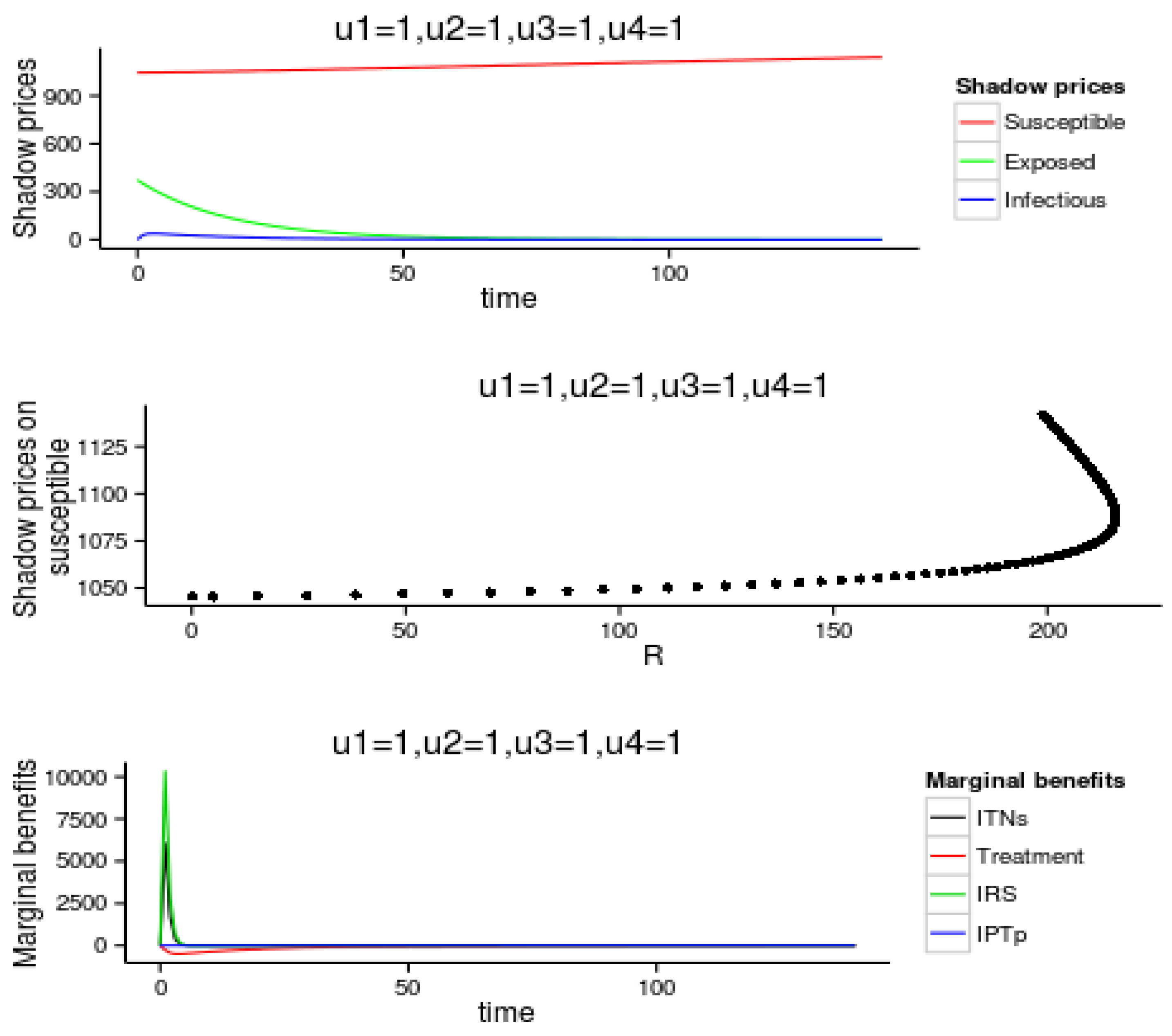
A case of the endemic epidemiological zone is used for the illustrative purpose. Numerical simulations showing the impact of the shadow prices (marginal value/cost) and marginal benefits by evaluating the shadow prices at the start of the malaria epidemic and as a function of the numbers of recovered or protected at the time of outbreak (susceptible human beings).

The marginal cost and effect of the intervention strategies are simulated for the Endemic transmission setting and the results are shown in Figure 2.

Simulations are also done for the epidemic, seasonal and low risks epidemiological zones.

Across all the four malaria transmission settings, it is observed that the marginal value (shadow price) of $I_h$ is much less damaging than the marginal values of $E_h$ and $S_h$. The shadow price on the susceptible humans are increasing overtime while the shadow prices of exposed starts dropping at $t=5$ days and shadow prices on infected starts dropping at $t=3$ days. In addition, across all the four malaria transmission settings, shows that the shadow price on $S_h$ starts at higher positive values, increases and stabilizes at higher prices closer to the total susceptible population. As more individuals recover from the disease the cost of the disease is still higher. It is also observed that across all the four malaria transmission settings shows that the marginal benefit of use of treatment is much smaller than the marginal benefit of IPTp, ITNs and IRS in that order. Smaller amounts of treatment is needed compared to IPTp, ITNs and IRS in that order to be able to eliminate the disease.

6.2. Numerical Simulation of the Optimal Malaria Control Strategies and Cost-Effectiveness Analysis

Numerical simulations are further done to show the infections averted and the cost associated with the infections averted by the intervention strategies for the four different transmission settings. Rankings of the number infections averted (effectiveness) is then done so that ICER can be applied.

For the different transmission settings we compute the optimal solution for the 15 strategies and their associated effectiveness $\overline{E}$ (infections averted) which is the difference between the numbers of infections when there is no intervention and when there are interventions. The strategies were classified as follows: ITN only (Strategy A), treatment only (Strategy B), IRS only (Strategy C), IPTp only (Strategy D), treatment and ITNs (Strategy E), ITNs and IRS (Strategy F), ITNs and IPTp (Strategy G), treatment and IRS (Strategy H), treatment and IPTp (Strategy I), IPTp and IRS (Strategy J), ITNs, treatment and IRS (Strategy K), ITNs, treatment and IPTp (Strategy L), ITNs, IRS and IPTp (Strategy M), IRS, treatment and IPTp (Strategy N), ITNs, treatment, IRS and IPTp (Strategy O). Based on the model simulation results, the strategies practiced in Kenya for different epidemiological settings were ranked in the order of increasing effectiveness.

The infections averted and cost of the intervention used is used to determine the cost-effectiveness of different combinations of the four intervention strategies using the ICER. We determined the total cost of the combined intervention strategies and the infections averted for different transmission settings.

The ICER for every two competing strategies for each epidemiological scenario is calculated and this shows the cost effectiveness for each strategy. The cost-effectiveness calculations are further verified using the computation of incremental cost-effectiveness ratios in table form for each epidemiological zone in order to have a complete overview of the outcome.

The

Table 6. Intervention strategies and its corresponding infections averted plus cost for Endemic region.

Strategies	Infections Averted	Cost
C	0.0000121135	0.00001817024
A	1.687	5.0613
F	1.6871	7.59196
G	3.68444	20.2644
M	3.6876	4.337343
D	5.35895	13.339738
J	5.368965	21.47586
I	101.7332	57.7995
N	101.7393	610.4358
L	102.8135	771.1012
O	102.818	925.3622
B	105.2167	210.4334
H	105.2167	368.2585
E	106.301	531.5846
K	106.3167	691.0584

below summarizes the ranking of simulation results on the effectiveness (infections averted) and the total costs by the different strategies for endemic scenario in Kenya.

The ICER for every two competing strategies was calculated and the results are presented in

Table 7. Incremental cost-effectiveness ratios of all combined strategies for Endemic region.

Strategy	Strategy Effects (E)	Cost ($) (C)	Incremental Cost ($\Delta C$)	Incremental Effect ($\Delta E$)	ICER ($\Delta C$)/($\Delta E$)
C	0.0000121135	0.00001817024	0.00001817024	0.0000121135	1.499999
A	1.687	5.0613	5.06128183	1.686987887	3.000189
F	1.6871	7.59196	2.53066	0.000099999	25306.6
G	3.68444	20.2644	12.67244	1.99734	6.344658
M	3.6876	4.337343	−15.927057	0.00316	−5040.21
D	5.35895	13.339738	9.002395	1.67135	5.386301
J	5.368965	21.47586	8.136122	0.010015	812.3936
I	101.7332	57.7995	36.32364	96.364235	0.376941
N	101.7393	610.4358	552.6363	0.0061	90596.11
L	102.8135	771.1012	160.6654	1.0742	149.5675
O	102.818	925.3622	154.261	0.0045	34280.22
B	105.2167	210.4334	−714.9288	2.3987	−298.048
H	105.2167	368.2585	157.8251	0	Inf
E	106.301	531.5846	163.3261	1.0843	150.6281
K	106.3167	691.0584	159.4738	0.0157	10157.57

.

Alternatives that are more expensive and less ineffective are excluded (A, F, D, J, N, O and H). These are the strategies that have higher ICER when compared. Having excluded strategy A, F, D, J, N, O and H, ICERs are recalculated for the remaining strategies (C, G, M, I, L, B, H and K) and are shown in

Table 8. Exclusion of more costly and less effective intervention strategies for Endemic region.

Strategy	Strategy Effects (E)	Cost ($) (C)	Incremental Cost ($\Delta C$)	Incremental Effect ($\Delta E$)	ICER ($\Delta C$)/($\Delta E$)
C	0.0000121135	0.00001817024	0.00001817024	0.0000121135	1.499999
G	3.68444	20.2644	20.26438183	3.684427887	5.500008
M	3.6876	4.337343	−15.927057	0.00316	−5040.21
I	101.7332	57.7995	53.462157	98.0456	0.545278
L	102.8135	771.1012	713.3017	1.0803	660.2811
B	105.2167	210.4334	−560.6678	2.4032	−233.301
E	106.301	531.5846	321.1512	1.0843	296.183
K	106.3167	691.0584	322.7999	1.1	293.4545

.

The dominated strategies (G, I, L and K) are then excluded and the ICERs are recalculated again (

Table 9. Exclusion of dominated alternative intervention strategies for Endemic region.

Strategy	Strategy Effects (E)	Cost ($) (C)	Incremental Cost ($\Delta C$)	Incremental Effect ($\Delta E$)	ICER ($\Delta C$)/($\Delta E$)
C	0.0000121135	0.00001817024	0.00001817024	0.0000121135	1.499999
M	3.6876	4.337343	4.33732483	3.687587887	1.176196
B	105.2167	210.4334	206.096057	101.5291	2.029921
E	106.301	531.5846	321.1512	1.0843	296.183

). These are the strategies that have higher ICER when compared.

In Table 9 the most cost effective quadrant will be strategy M and strategy B and in deciding between them the size of the available budget must be brought to bear. Strategy M is the combination of ITNs, IRS and IPTp while strategy B is the use of treatment only.

Repeating the same procedure for the remaining epidemiological zones (epidemic, seasonal and low), the findings shows that for the endemic regions the combination of ITNs $u_1$, IRS $u_3$, and IPTp $u_4$ is the most cost-effective of all the combined strategies developed in this study for malaria disease control and prevention; for the epidemic prone areas is the combination of the treatment $u_2$, and IRS $u_3$; for seasonal areas is the combination ITNs $u_1$ plus treatment $u_2$; and for the low risk areas is the use of treatment $u_2$ only. The result confirms the role which the four intervention strategies are playing in order to eradicate or minimize the spreading of the malaria disease.

7. Discussion

This paper conducted cost effective analysis of one or all possible combinations of malaria control strategies for different transmission settings in order to assess the extent to which the intervention strategies are beneficial and cost effective. For the four different transmission settings the optimal control model simulation was done for the 15 strategies and their associated effectiveness $\overline{E}$, which is the difference between the numbers of infections when there is no intervention and when there are interventions, was used to rank the effectiveness of the interventions [7,8]. The marginal costs and benefits have also been investigated. ICER was then used to compare the health and economic benefits of the intervention strategies. Numerical simulation compared the marginal value and marginal effect for the four intervention strategies [8] across the four different transmission settings.

The findings of the study shows that for the endemic regions the combination of ITNs, IRS, and IPTp was the most cost-effective of all the combined strategies developed in this study for malaria disease control and prevention. This findings are different from the findings of Okosun et al. [8], who found that the combination of the spray of insecticides and treatment of infective individuals were the cost effective strategies. This may be due to the fact that in our study we considered the at most risk groups while in the Okusun et al. [8] they considered whole population. The findings shows that preventive measures tends to have a greater health benefit in a cost effective or economical manner in minimizing malaria transmission for the most at risk groups. Stuckey et al. [5] showed that increasing coverage of vector control interventions (preventive strategies) had a larger simulated impact compared to adding treatment measures.

Our results shows that for the epidemic prone areas the cost effective strategy was the combination of the treatment and IRS which agrees with Okosun et al. [8]. This is because the combination of the preventive and treatment actions tend to be more effective in the reduction of parasitic prevalence to below 1% [32]. This is due to the fact that infected mosquito population is reduced by IRS and the infected human population is reduced via the treatment.

For seasonal areas, the findings of this study showed that the combination ITNs and treatment would be the most cost effective intervention strategy to reduce malaria transmission among the under-five and the pregnant women. This is slightly different with the findings of Griffin et al. [30] who found that for the high seasonal transmission settings the use of LLITNs, IRS and treatment would help reduce the transmission of malaria.

The results showed that for the low risk areas is the use of treatment only. These findings were different from Hansen et al. [9] who found that the most cost effective strategy was the use of ITNs alone in Uganda low transmission settings.

The result confirms the role which the four intervention strategies are playing in order to eradicate or minimize the spreading of the malaria disease among the at risk groups. The policy implications of these findings is that different transmission settings require different interventions that are health beneficial and cost effective. The results can guide decision makers in making more informed and evidence-based choices on the health resources being allocated. These findings may help inform the development of guidelines for prevention of malaria among the under-five and the pregnant women in different transmission settings in Kenya as well as in other African countries.

These findings were based on the use of secondary data, a more designed study may be needed to ascertain the findings of these studies. Including other possible positive externalities would improve the cost-effectiveness of interventions strategies.

8. Conclusions

In this manuscript, we formulated and analyzed a deterministic model for malaria transmission that incorporated the intervention strategies for the most at risk groups for malaria (pregnant women and children under five years of age). Optimal control analysis of the model and cost effectiveness analysis of the optimal control strategies has also been performed. Some of the main theoretical and epidemiological findings can be summarized as follows:

• The disease free equilibrium point for System (1) is locally asymptotically stable whenever the reproduction number, $R_0<1$ and unstable if $R_0>1.$
• The sensitivity analysis showed that the main sensitive parameters to $R_0$ across all the settings was the mosquito’s natural death rate, ${\mu }_m$, and mosquito biting rate, $ϵ$, this was followed by the by the mosquito contact rate with humans, $\varphi$, probability of mosquito getting infected, $\lambda$, the probability of humans getting infected, $\beta$, and the recruitment rate of mosquitoes and humans.
• The numerical simulations and cost-effectiveness analysis showed that the most cost-effective strategies for malaria disease control and prevention for the endemic regions was the combination of ITNs, IRS, and IPTp; for the epidemic prone areas is the combination of the treatment and IRS; for seasonal areas is the use of ITNs plus treatment; and for the low risk areas is the use of treatment only.
• The results also demonstrated that malaria transmission in Kenya can be minimized through tailor-made intervention strategies for malaria control which produces health improvements in the most cost effective way for different epidemiological zones. This will provide basis for informed decision making about the value for money for the public health programs and can guide in the allocation of malaria control resources for the post-2015 malaria eradication strategies and the achievement of the Sustainable Development Goals.

References

1. World Health Organization. World Malaria Report 2014; World Health Organization, Global Malaria Programme: Geneva, Switzerland, 2014; Available online: http://www.who.int/mediacenter/factsheets/fs094/en/ (accessed on 20 March 2015).
2. Guerra, C.; Gikandi, P.; Tatem, A.; Noor, A.; Smith, D. The limits and intensity of Plasmodium falciparum transmission: Implications for malaria control and elimination worldwide. PLoS Med. 2008, 5, e38. [Google Scholar] [CrossRef] [PubMed] [Green Version]
3. Division of Malaria Control. National Guidelines for Diagnosis, Treatment and Prevention of Malaria in Kenya, 3rd ed.; Division of Malaria Control (Ministry of Public Health and Sanitation): Nairobi, Kenya, 2010. [Google Scholar]
4. White, M.; Conteh, L.; Cibulskis, R.; Ghani, A. Costs and cost-effectiveness of malaria control interventions—A systematic review. Malar. J. 2011, 10, 337. [Google Scholar] [CrossRef] [PubMed]
5. Stuckey, E.M.; Stevenson, J.; Galactionova, K.; Baidjoe, A.Y.; Bousema, T.; Odongo, W.; Kariuki, S.; Drakeley, C.; Smith, T.A.; Cox, J.; et al. Modeling the Cost Effectiveness of Malaria Control Interventions in the Highlands of Western Kenya. PLoS ONE 2014, 9, e107700. [Google Scholar] [CrossRef] [PubMed] [Green Version]
6. Phillips, C. What Is Cost-Effectiveness? Health Economics. 2009. Available online: http://www.medicine.ox.ac.uk/bandolier/painres/download/whatis/Cost-effect.pdf (accessed on 18 August 2014).
7. Rodrigues, P.; Silva, C.J.; Torres, D.F.M. Cost-Effectiveness Analysis of Optimal Control Measures for Tuberculosis. Bull. Math. Biol. 2014, 76, 2627–2645. [Google Scholar] [CrossRef] [PubMed]
8. Okosun, K.; Rachid, O.; Marcus, N. Optimal control strategies and cost-effectiveness analysis of a malaria model. BioSystems 2013, 111, 83–101. [Google Scholar] [CrossRef] [PubMed]
9. Hansena, K.S.; Ndyomugyenyib, R.; Magnussenc, P.; Clarked, S.E. Cost-effectiveness analysis of three health interventions to prevent malaria in pregnancy in an area of low transmission in Uganda. Int. Health 2012, 4, 38–46. [Google Scholar] [CrossRef] [PubMed]
10. Le Port, A.; Cottrell, G.; Dechavanne, C.; Briand, V.; Bouraima, A.; Guerra, J.; Choudat, I.; Massougbodji, A.; Fayomi, B.; Migot-Nabias, F.; et al. Prevention of malaria during pregnancy: Assessing the effect of the distribution of IPTp through the national policy in Benin. Am. J. Trop. Med. Hyg. 2011, 84, 270–275. [Google Scholar] [CrossRef] [PubMed]
11. Parise, M.E.; Ayisi, J.G.; Nahlen, B.L.; Schultz, L.J.; Roberts, J.M.; Misore, A.; Muga, R.; Oloo, A.J.; Steketee, R.W. Efficacy of sulfadoxine-pyrimethamine for prevention of placental malaria in an area of Kenya with a high prevalence of malaria and human immunodeficiency virus infection. Am. J. Trop. Med. Hyg. 1998, 59, 813–822. [Google Scholar] [PubMed]
12. Shulman, C.E.; Dorman, E.K.; Cutts, F.; Kawuondo, K.; Bulmer, J.N.; Peshu, N.; Marsh, K. Intermittent sulphadoxine-pyrimethamine to prevent severe anaemia secondary to malaria in pregnancy: A randomised placebo-controlled trial. Lancet 1999, 353, 632–636. [Google Scholar] [CrossRef]
13. Rogerson, S.J.; Chaluluka, E.; Kanjala, M.; Mkundika, P.; Mhango, C. Intermittent sulfadoxine-pyrimethamine in pregnancy: Effectiveness against malaria morbidity in Blantyre, Malawi, in 1997–99. Trans. R. Soc. Trop. Med. Hyg. 2000, 94, 549–553. [Google Scholar] [CrossRef]
14. Otieno, G.; Koske, J.K.; Mutiso, J.M. A Model for Malaria Transmission Dynamics with Interventions Strategies in Kenya. 2015. submitted. [Google Scholar]
15. Van den Driessche, P.; Watmough, J. Reproduction numbers and sub-threshold endemic equilibria for compartmental models of disease transmission. Math. Biosci. 2002, 180, 29–48. [Google Scholar] [CrossRef]
16. Flores, J.D. Mathematical Modelling, 4.5 Routh-Hurwitz Criteria; Department of Mathematical Sciences, The University of South Dakota: Vermillion, SD, USA, 2011. [Google Scholar]
17. Chitnis, N.; Cushing, J.; Hyman, J. Bifurcation analysis of a mathematical model for malaria transmission. SIAM J. Appl. Math. 2006, 67, 24–45. [Google Scholar] [CrossRef]
18. Pontryagin, L.; Boltyanskii, V.G.; Mishchenko, E. The Mathematical Theory of Optimal Processes; Wiley: New York, NY, USA, 1962. [Google Scholar]
19. Adams, B.M.; Banks, H.T.; Kwon, H.; Tran, H.T. Dynamic multidrug therapies for HIV: Optimal and STI control approaches. Math. Biosci. Eng. 2004, 1, 223–241. [Google Scholar] [PubMed]
20. Mwamtobe, P.; Abelman, S.; Tchuenche, J.; Kasambara, A. Optimal (Control of) Intervention Strategies for Malaria Epidemic in Karonga District, Malawi. Abstr. Appl. Anal. 2014, 2014, 1–20. [Google Scholar] [CrossRef]
21. Joshi, H.R. Optimal control of an HIV immunology model. Optim. Control Appl. Math. 2002, 23, 199–213. [Google Scholar] [CrossRef]
22. Fleming, W.H.; Rishel, R.W. Deterministic and Stochastic Optimal Control; Springer Verlag: New York, NY, USA, 1975. [Google Scholar]
23. Felippe de Souza, J.A.M.; Marco, A.L.C.; Takashi, Y. Optimal control theory applied to the anti-viral treatment of AIDS. In Proceedings of the Conference on Decision and Control, Sydney, Australia, 12–15 December 2000.
24. Otieno, G.; Koske, J.K.; Mutiso, J.M. Optimal Control Strategies for the Spread of Malaria in Kenya. 2015. submitted. [Google Scholar]
25. Lenhart, S.; Workman, J.T. Optimal Control Applied to Biological Models; Chapman and Hall/CRC: London, UK, 2007. [Google Scholar]
26. Kenya National Bureau of Statistics. Kenya Population and Housing Census 2009; KNBS, Ministry of Planning, National Development and Vision 2030: Nairobi, Kenya, 2010. [Google Scholar]
27. Kbenesh, B.; Yanzhao, C.; Hee-Dae, K. Optimal control of vector-borne diseases: Treatment and prevention. Discret. Contin. Dyn. Syst. Serv. B 2009, 11, 587–611. [Google Scholar]
28. Niger, A.M.; Gumel, A.B. Mathematical analysis of the role of repeated exposure on malaria transmission dynamics. Differ. Equ. Dyn. Syst. 2008, 16, 251–287. [Google Scholar] [CrossRef]
29. Chiyaka, C.; Tchuenche, J.M.; Garira, W.; Dube, S.A. Mathematical analysis of the effects of control strategies on the transmission dynamics of malaria. Appl. Math. Comput. 2008, 195, 641–662. [Google Scholar] [CrossRef]
30. KNBS and ICF Macro. Kenya Demographic and Health Survey, 2008–2009; Kenya National Bureau of Statistics (KNBS) and ICF Macro: Calverton, Maryland, 2010. [Google Scholar]
31. R Development Core Team. R: A Languange and Environment for Statistical Computing; R Foundation for Statistical Computing: Vienna, Austria, 2011. [Google Scholar]
32. Griffin, J.; Hollingsworth, T.; Okell, L.; Churcher, T.; White, M.; Hinsley, W.; Ghani, A. Reducing Plasmodium falciparum malaria transmission in Africa: A model-based evaluation of intervention strategies. PLoS Med. 2010, 7, e1000324. [Google Scholar] [CrossRef] [PubMed] [Green Version]
Figure 1. Malaria model with interventions.
Mathematics 04 00014 g001
Figure 2. Numerical simulations of the economic evaluations of the malaria model for the endemic transmission settings.
Mathematics 04 00014 g002