Abstract
Renewable energy systems (RESs) have introduced themselves as vital solutions for energy supply in remote regions, wherein main utility supply systems are not available. The construction of microgrid (MG) systems is useful candidate for proper control and management with hybrid RESs. However, RESs-based MGs face reduced power system inertia due to the dependency of RESs on power electronic converter systems. Accordingly, preserving nominal operating frequency and reduced deviations in tie-line power are crucial elements for proper operation of interconnected MGs in remote areas. To overcome this problem, load frequency control (LFC) systems have proven featured solutions. Therefore, this paper proposes a new non-integer LFC method based on the fractional order (FO) control theory for LFC in interconnected MGs in remote areas. The proposed control is based on the three degree of freedom (3DoF) cascaded 1+proportional-integral-derivative-accelerated (PIDA) controller with FOPI controller, namely 3DoF 1+PIDA/FOPI LFC scheme. The proposed 3DoF 1+PIDA/FOPItakes the advantages of the accelerated term of PIDA control to improve power system transients, regarding maximum overshoot/undershoot and settling times. Additionally, it employs outer loop to reduce errors and faster inner loop to mitigate disturbances effects. The contribution of plug-in controlled electric vehicles (EVs) are considered to enhance the frequency regulation functions. An optimized design of the proposed 3DoF 1+PIDA/FOPI LFC scheme is proposed using the newly developed hybrid equilibrium optimizer (EO)-slime mould optimization (SMA) algorithm (namely EOSMA optimizer). The EOSMA combines the features of the EO and SMA powerful optimization algorithms. A two interconnected MGs in remote areas with RESs and EVs inclusions with high penetration levels is selected to verify the proposed 3DoF 1+PIDA/FOPI LFC scheme and the EOSMA optimizer. The results show high ability of the proposed controller and design scheme to minimize MGs’ frequency and tie-line power fluctuations and to preserve frequency stability and security.
Keywords:
electric vehicles (EVs); equilibrium optimizer; load frequency control; non-integer controllers; slime-mould algorithm; renewable energy; remote microgrids MSC:
68N30
1. Introduction
Remote area communities face the challenges of limited energy access of fossil fuels. The energy transition and the direction to replace the conventional fossil fuels with existing everywhere renewable energy sources (RESs) have become important needs [1]. Moreover, the various installed distributed generation systems can be connected forming isolated and/or interconnected microgrid (MG) systems [2]. However, the constructed MGs suffer from RESs’ intermittent nature and the continuous reduction in power system inertia. The main reason behind the inertia reduction is their dependency on power electronics converters, which lack inertia compared to conventional generations [3]. Therefore, connecting energy storage systems has become essential in RESs-based interconnected MGs in remote communities. With the recent replacements of electric vehicles (EVs), their inherent battery storage systems can be employed for this function without adding more energy storage devices [4].
Properly-designed and selected control schemes can achieve enhanced performance of interconnected remote MGs, especially with considering the associated problems to RESs and benefits from EV systems [5]. The load frequency control (LFC) schemes have been widely introduced in the literature for solving frequency and tie-line regulations of single/multiple areas power grid systems [6]. The LFC schemes are designed to be able to regulate the generated powers and to mitigate loads’ variations, parameters variations, intermittency of RESs, and MG disturbances. The controller type and design method are jointly determining MG response against various disturbances. Moreover, implementation complexity, and data requirements for design represent critical factors for selecting appropriate controller and design method [7].
Model predictive controller (MPCs) have been introduced in literature for various LFC applications [8]. In [9], robust MPC has been proposed for gate-controlled series-capacitor (GCSC) power grids based on using two cascaded nominal and ancillary MPCs. Moreover, robust sliding mode controllers (SMCs) LFC schemes have been presented in literature [10,11]. Other LFC schemes based on linear-matrix inequality (LMI) [12], and robust controllers [13,14] have been also presented in literature for LFC applications. Recently, machine learning (ML)-based LFC schemes have been proposed for LFC applications, such as the deep learning LFC [15], intelligent controllers [16], data-driven controllers [17], etc.
In [18,19], comparisons between classical and advanced LFC schemes have been introduced. The intelligent LFC schemes can improve the functionality of power grids and frequency stability. Although, some limitations exist due to their need for huge data for tuning processes, powerful computation processors, and complex and expert knowledge. In the other side, integer and non-integer classical LFC schemes are still finding wide concerns due to their simple implementations, easy to be understood, ability to be optimized using metaheuristic algorithms, etc. [19,20]. The main combinations of integer and non-integer LFC include the proportionals (P), integrals (I), tilts (T), derivatives (D), filters (F), fractional filters (FF), and fractional order (FO) operators.
The integer order LFC schemes have been introduced in the literature using the I, PI, PID, and IDD controllers [21,22]. Wherein metaheuristic optimization algorithms have been presented for their optimum design, such as artificial bee-colony algorithm (ABC) [23], Harris Hawks optimization algorithm (HHO) [21], and balloon-effects (BE) modulation [22]. An adaptive I-based LFC method optimized with Jaya-Balloon optimization (JBO) has been presented in [24]. Another robust PID LFC method has been presented in [25] and the imperialist-competitive algorithm (ICA) has been presented to optimally determine PID parameters. Moreover, the PID-based virtual inertia controller has been provided for enhancing inertial response of real power system case study [26]. The integer LFC schemes are simple, less complex, easy to design, and low cost for implementation. However, they fail at mitigating fluctuations at uncertain system parameters. A cascaded PD-PI LFC method has been presented in [27] with parameters optimization using enhanced slime-mould optimizer algorithm (ESMOA). Additionally, the driver-training based optimization (DTBO) has been proposed with the PI-PDF LFC method in [28]. Additional integer LFC schemes have been presented using PIDF [29,30], two degrees-of-freedom 2DoF-PID [31], cascaded PD with PID [32], PI-(1 + DD) [23], PID with double derivative (PID2D) [33], IPD-(1 + I) [34], fuzzy logic controller (FLC) and PID (FLC-PID) [35], and neuro-fuzzy controllers [36]. Some optimizer algorithms have been presented for optimizing their design, such as slap swarm optimizer algorithm (SSA) [37], and flower-pollination optimization algorithm (FPA) [38]. An optimal output feedback controller has been provided in [39] for a realistic power system case study. The presented controller showed robust performance against system uncertainty, parameters variations, and system’s non-linearity. Additionally, ultra-local modelling-based intelligent controllers have been presented in literature [40,41,42].
The accelerated term (double derivative) is added to integer PID control scheme to form the PID accelerated (PIDA) control scheme [43]. The accelerated term is capable of reducing overshoot values and settling time values due to the added second order derivative term. The PIDA has been introduced in [44] for isolated MGs. The coefficient diagram method (CDM) has been applied for designing the PIDA LFC scheme with preserving more stable performance of the power system. Another cascaded PIDA scheme has been applied in [45] for wave energy-based MGs. The cascaded structure of PIDA can enhance the disturbance rejection capabilities of MGs. The marine predator optimizer algorithm (MPA) has been presented for designing the cascaded PIDA LFC scheme. In [46], the various optimization methods have been applied for optimized PIDA using the teaching–learning-based optimizer (TLBO), harmony-search optimizer algorithm (HS), and the sine–cosine optimizer algorithm (SCA). Another supply–demand optimizer algorithm (SDOA)-based optimized PIDA controller has been introduced in [47] for LFC applications.
From another side, FOPID has been proposed for several case studies and it is joined with SCA optimizer [48], genetic algorithm (GA) [25], and movable damped wave algorithm (MDWA) [49]. A dual stage FOPID LFC scheme has been presented in [50] for stabilizing frequency deviations in standalone MGs. Another FOPID with filter (FOPIDF) has been proposed in [51,52]. The three DoF (3DOF-TID) is cascaded with FOPID in [53] for improving stability of MG systems. Another cascaded TID-FOPID has been introduced in [54] for GCSC devices. A cascaded FOID with FOPIDF (cascased FOID-FOPIDF) has been presented in [55] for improving the performance of existing cascaded non-integer LFC schemes. The cascaded FO-IDF [56], TID [54], cascaded PI-TDF [57], and TIDF [58] have been also proposed in literature for LFC. Some optimization algorithms have been presented for optimizing control parameters, such as pathfinder optimizer algorithm (PFA) [59], ABC algorithm [60], differential evolution optimizer (DE) [58], and slap–swarm optimizer algorithm (SSA) [57]. In [61], the ITDF optimized with imperialist competitive optimizer algorithm (ICA) has been proposed for multi-MG power systems.
Furthermore, some modified non-integer LFC schemes have been introduced in the literature. A hybrid non-integer LFC scheme using FOPID with TID has been presented in [62] with considering installed EVs in the system. The design optimization is achieved through applying the artificial ecosystem optimization algorithm (AEO). Another modified controller has been presented in [54] for the GCSC-based interconnected MGs. An enhanced controller with superconducting-energy storage systems (SMES)-based MGs has been introduced in [63]. The combined hybrid non-integer with TIDF has been introduced in [64] with optimum LFC design. The butterfly optimizer algorithm (BOA) [65], barnacle-mating optimization (BMO) [66], and manta ray-foraging optimizer algorithm (MRFO) [63] have been applied in their optimization process. The FLC is combined in the literature with non-integer LFC schemes, such as the cascaded FLC-FOPID in [67], FLC-FOPI-FOPD [68], FL-FOPIDF [69], FPIDN-FOPIDN [56], and FLC-PIDF-FOI [70].
It can be seen from literature that wide control schemes have been introduced for LFC with different structures. In addition, vast optimization techniques have been jointly applied in literature for optimizing LFC parameters. With the expected high RESs’ penetration levels in remote interconnected MGs, the joint use of LFC schemes and optimization methods is important for enhancing frequency stability in remote interconnected MGs. The appropriate selection of the LFC scheme and its optimized parameters are crucial for the mitigation of expected transients, especially with the reduced MG inertia due to RESs’ inclusions at large scales. Another issue of applied metaheuristic optimization methods is through lacking reliability due to probable settling at their local minimum [71]. Additionally, efficient tuning of non-integer LFC schemes is important for benefiting their added degree of freedom compared to their integer LFC counterparts [72]. It is also important to consider the long elapsed time, high sensitivity for parameters variation, long time for computations, and saturation of some applied optimization algorithms. Therefore, this paper proposes a new non-integer LFC scheme based on the 3DoF cascaded (1+PIDA)/FOPI LFC scheme optimized with the hybrid equilibrium optimizer (EO) with a slime mould algorithm (SMA) optimizer (EOSMA) [73] for enhancing frequency stability of remote interconnected MGs with high RESs and EV penetration levels.
The EOSMA optimizer merges the benefits of powerful EO [74] and SMA [75] optimizers and, hence, it is selected in this paper. The main characteristics of EOSMA behind its superior performance are the following [73].
- The EOSMA has better explorations and exploitation capabilities than SMA and EO optimizers due to using greedy selection strategy, hierarchical partitioning strategy, differential mutation strategy, and the boundary checking strategy. The exploitation capability is enhanced through the greedy selection strategy and the boundary checking mechanism. Whereas exploration capability is enhanced through hierarchical partitioning strategy and the differential mutation strategy.
- In EOSMA, a low-efficiency anisotropic searching operator of SMA optimizer is replaced with highly-efficient concentration updating operator of the EO optimizer. Thence, the concentrations of slime moulds are balanced in all of the directions and consequently it is able to improve searching efficiency of EOSMA optimizer.
- In EOSMA, random differential mutation strategy is introduced, which enables an EOSMA optimizer to avoid local optimums and premature convergence.
- In EOSMA, invalid searching is excluded due to its improvements of boundary checking. The searching boundary in EOSMA is updated for solution vectors beyond searching boundaries to current solution’s midpoint.
Consequently, EOSMA is introduced in this paper for optimizing parameters of LFC schemes based on its aforementioned characteristics and benefits. The main contribution of this article is summarized as the following.
- A new optimized non-integer LFC scheme is proposed for frequency regulation in remote interconnected MGs with high penetration levels of RESs and EVs. The proposed control method can effectively mitigate various fluctuations in RESs’ based MG systems.
- The proposed controller is based on new 3DoF 1+PIDA/FOPI controller, which employs three different input signals (frequency deviation, tie-line power, and area control error) in each area. The use of three signals is advantageous at mitigating various low frequency in addition to high-frequency-based disturbances.
- The proposed 3DoF 1+PIDA/FOPI controller improves the frequency regulation performance compared with widely-presented PID, PIDA, 1+PIDA, and 1+PID/FOPI controllers while disturbances rejection capability is enhanced.
- An improved LFC structure is proposed for remote area through using 1+PIDA controller cascaded with FOPI in the feedforward loop. The proposed structure can mitigate the various existing frequency and tie-line power deviations due to using two cascaded control loops.
- The proposed 3DoF 1+PIDA/FOPI controller is general and can be applied to various case studies of MG systems with any number of interconnected areas.
- The EV participation in frequency regulation is achieved in this paper through employing the proposed centralized structure of the cascaded 3DoF 1+PIDA/FOPI controller. Thence, the proposed 3DoF 1+PIDA/FOPI controller achieves reduced control complexities due to the centralized structure with coordination between EVs and LFC systems.
- A new application of the newly developed equilibrium optimizer (EO)-slime mould optimization (SMA) algorithm (namely EOSMA) is proposed for optimizing the proposed cascaded 3DoF 1+PIDA/FOPI controller. The EOSMA merges the advantages of two powerful optimization algorithms, the EO and the SMA optimizers. Optimum LFC parameters are simultaneously-determined using the EOSMA optimizer to minimize the desired control objectives.
The paper is organized in the following way. Section 2 presents the mathematical representation models of remote MG systems. The non-integer control modelling and the proposed 3Dof 1+PIDA/FOPI control scheme are detailed in Section 3. The proposed optimization procedures and EOSMA optimizer are presented in Section 4. Section 5 shows the obtained results of the selected case study remote MG system. Finally, conclusions of paper are introduced in Section 6.
2. Modelling of Interconnected Remote MGs
2.1. Interconnected MGs Structure
The structure of selected remote interconnected MGs case study is shown in Figure 1. The MG system is divided into two interconnected areas linked by AC tie-line. The MG system is divided to construct two interconnected areas, namely area a, and area b, respectively. The main components in area a are the thermal plant, locally-connected loads, EVs, and wind plant. Whereas the main components in area b are the hydraulic plant, locally-connected loads, EVs, and photovoltaic (PV) plant. In this MG system, EVs are assumed to be equally-distributed between the two interconnected MGs.
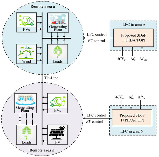
Figure 1.
Components of the studied interconnected remote MGs with installed EVs.
2.2. Thermal and Hydraulic Plants Modelling
The most common model of thermal plant is through using first order transfer function for the governor and for the turbine . Their representations are as following [76]
where and denote time constants of governor side, and turbine side, respectively. Furthermore, the hydraulic plant representation is the following [63]:
where , , are the time constants for the governor, transient droop, and the governor’s reset-time, respectively, and denotes starting time of water’s penstocks. In the proposed analysis and obtained results, the the generation rate constraint (GRC) and governor dead-band (GDB) are considered as shown in Figure 2.
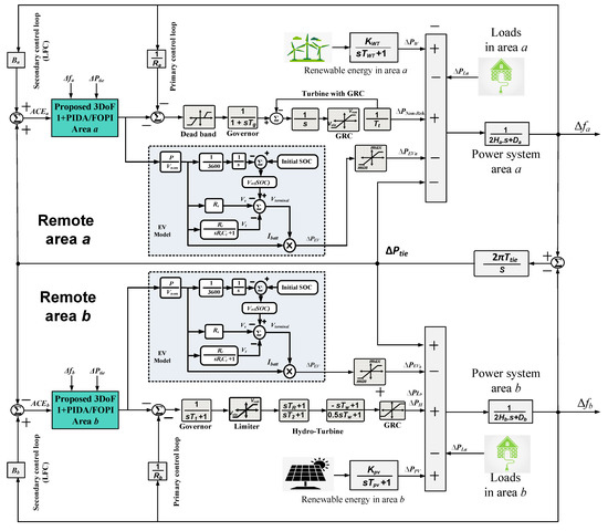
Figure 2.
Complete remote interconnected MGs’ model.
2.3. PV and Wind Plant Modelling
The operating point of PV plants depends on the solar irradiance and ambient temperature of solar PV panels. The irradiance variations result in making unpredictable outputted power from PV plants. Power electronics-based conversion systems have become a main part of PV systems to ensure continuous tracking of maximum power. Moreover, they perform the grid integration functionality with injecting high-power quality currents’ waveforms. Therefore, outputted power variations possess negative impacts on power systems stability performance. The outputted power modelling from PV plants is expressed as the following [77,78]
where stands for PV panel’s conversion efficiency (in %), stands for solar insolation (W/m), S stands for PV area (m), and represents ambient temperature (C). A realistic PV outputted power is implemented in this paper for representing PV intermittent characteristics based on the model from [79].
Additionally, a first order transfer function is employed for PV and wind plants. The PV plant model representation is as following [78]
where and denote time constant, and gain of PV model, respectively.
From another side, the outputted mechanical wind turbine power has also wind speed related power fluctuations, which represents the main source for wind plants’ intermittent nature. The wind power can be represented as following [77,78]
where stands for air density (kg/m), represents swept area (m), stands for power coefficient, and denotes to wind speed (m/s). A realistic wind outputted power is implemented in this paper for representing wind intermittent characteristics based on the model from [79]. The model representation of is as following [78]
where and , denote time constant and gain of wind plant, respectively.
2.4. Installed EVs Model
The recent replacements of EVs in power grids instead of traditional vehicles give the chance to utilize their inherent batteries. Thence, installed EVs’ batteries can be directed to enhance frequency regulation functionality in the interconnected remote MGs. In addition, EVs eliminates the need for additional energy storage devices in those systems [62]. Accordingly, EVs can lead to reducing systems’ costs and to improving remote MGs operation. Modelling the dynamics and behavior of EVs’ energy storage is principal task for better sizing, management, control, and evaluations to perform various possible tasks in power systems. For instance, Volterra integral equations based energy storage modelling have shown improved performance in several applications, such as energy management, unit commitment, forecasting, etc. [80,81,82,83]. For modelling the functionality of EVs in LFC, the equivalent Thevenin-based EV model, which has become common for LFC studies [84,85], is implemented and integrated to the two-area MG system. This model includes representing open-circuited battery voltage. This voltage is depending on the batteries’ state of charges (SOCs) of EVs . A series resistance and parallel RC network (, ) are added to the model to represent ohmic losses and transients of batteries, respectively. The voltage is expressed through the Nernst equation as the following [86]
where denote nominal battery voltage, and denote nominal battery capacity (Ahr). Whereas S represents parameters’ sensitivity of , T denote temperature, F and R denote constants of Faraday and gas, respectively. The model parameters of installed EVs are included in Table 1, wherein limiting maximum and minimum of EV power are set at ±0.1 p.u. MW to limit injected powers from installed EVs.

Table 1.
Interconnected MGs’ parameters for system modelling (), [87].
2.5. State Space Modelling of Remote MGs
Figure 2 shows the complete interconnected MGs’ model, including EVs and RESs. The system parameters for the selected case study are shown in Table 1 based on the data in [63,85]. The state space represents a general linearized model for LFC studies. It can be expressed as following
where x includes vector of state variables, y includes vector of output states, includes vector of existing system disturbances, and u includes vector of control outputs.
The vectors x, and are the following:
The vector u includes the outputs of LFC signals in both areas , and , respectively, and the supplied power from EVs ( and ). It is the following
The matrices of the state space model (A, , , and C) are determined by system parameters, as shown in Figure 2. They are expressed as the following:
3. Proposed Non-Integer LFC Scheme
3.1. The Non-Integer Calculus
The non-integer calculus is based on the FO representation theory. The most common definitions of the non-integer calculus are the Grunwald–Letnikov scheme, Riemann–Liouville scheme, and Caputo scheme [88]. In Grunwald–Letnikov scheme, non-integer derivative of the function f within the limits from a to t is defined as following [89]
where h stands for step time, and represents operator for only integer terms in Grunwald–Letnikov scheme. Whereas n has to satisfy that (). The binomial coefficients are defined as the following [89]
where gamma function in (18) is commonly defined as [88]:
Riemann-Liouville have defined non-integer derivatives with avoiding the usage of sums and limits. While it employs integer derivatives and integrals representations as the following [90]:
Another way to define non-integer derivatives has been introduced by Caputo as the following [89]:
A general non-integer operator form for representing various non-integer control terms as the following:
The Oustaloup-based recursive approximations (ORA) of non-integer derivatives have confirmed suitable representations of non-integer control schemes, especially for real-time-based digital implementations [88]. The ORA representation has been widely-used for optimizer determination of non-integer control schemes, thence it is utilized in this paper for modelling the proposed non-integer LFC scheme. The approximated mathematical representations of th non-integer derivatives () are the following [88],
where and are poles locations, and zeros locations of sequence. They are calculated using the following representations
where approximated non-integer operators functions have number of poles/zeros. Thence, N determines the order of ORA representation with order equals to . In this article, ORA is utilized with considering inside frequency limits () between rad/s.
3.2. Featured LFC Schemed from Literature
As clarified in the introduction section, several integer and non-integer LFC schemes have been introduced in literature. Figure 3 shows some featured LFC schemes from literature (wherein colored blocks are used for tunable parameters). The mathematical representation of LFC schemes can be represented in the following way:
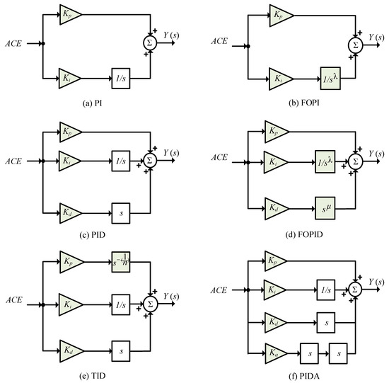
Figure 3.
Featured LFC schemes from literature (wherein colored blocks are used for tunable parameters).
From (27) and Figure 3, it is clear that integer PI LFC has only two tunable parameters, whereas non-integer FOPI has three tunable parameters. The integer PID, and PIDF LFC schemes have three and four tunable parameters, compared with five in non-integer FOPID and six in non-integer FOPIDF LFC schemes. The non-integer TID and TIDF have four and five tunable control parameters, respectively. This, in turn, confirms the added degrees-of-freedom in non-integer LFC schemes compared with integer LFC schemes. Thence, the proposed controller in this paper is relying on non-integer FO theory. Whereas, PIDA and 1+PIDA LFC schemes can be represented as the following:
3.3. Proposed 1+PIDA/FOPI LFC Scheme
The control structure of proposed 1+PIDA-FOPI scheme is shown in Figure 4 for each remote MG system. The proposed 1+PIDA/FOPI LFC scheme is based on cascaded 1+PIDA control in the first loop with FOPI in the second loop. Thence, it is capable of combining best properties from 1+PIDA and FOPI with achieving fast response, robust control, and better rejection of disturbances. Additionally, the feedforward control loop includes sensed signals from frequency deviation and tie-line power in local remote area. The input ACE signals (, and ) as inputs signals to and , respectively, for 1+PIDA control loop are mathematically expressed as
where stands for capacities’ ratio between remote areas a and b. Whereas outputs and of 1+PIDA control loop are represented as:
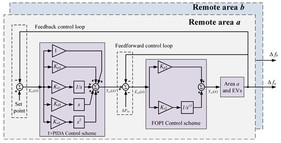
Figure 4.
Proposed 3DoF 1+PIDA/FOPI LFC scheme.
Therefore, each remote MG contains four tunable control parameters in the first loop as in (30). Remote area a needs designing four parameters (, , , and ) in the 1+PIDA control loop, whereas remote area b needs designing (, , , and ). The second FOPI loop is feed by the output of the 1+PIDA control loop. The input error signals and for the second FOPI loops are as the following:
The FOPI loops are mathematically expressed as:
Thence, the FOPI loop has three tunable parameters in remote area a with designing (, , and), and remote area b needs determining (, , and).
4. The Proposed EOSMA-Based Parameters Optimization
4.1. Optimization Procedures
Improved and more stable operation of interconnected remote MGs can be achieved through proper design and selection of LFC scheme parameters. The proposed 3DoF 1+PIDA/FOPI LFC scheme has seven tunable control parameters in each remote area. The determination and tuning procedures of all 14 parameters in the two areas are made in simultaneous way to guarantee the desired control objectives. The four featured in the objective function formulation literature are:
- Integral-squared-error (ISE)
- Integral-time squared-error (ITSE),
- Integral-absolute-error (IAE),
- Integral-time absolute-error (ITAE)
The objectives of control design in remote areas are preserving minimum deviations in each remote area frequency (minimize and ), in addition to preserving minimized fluctuations in the tie-line power between remote areas (minimize ). Then, they are formulated to construct the overall control fitness function. Based on (33)–(36), the ISE, ITSE, IAE, and ITAE fitness functions are formulated for the proposed optimization procedures as:
Accordingly, the proposed optimization procedure includes 14 parameters to be tuned for preserving minimized fitness function. The limiting constraints for the optimization procedures are the controllers’ parameters as the following,
wherein, represents LB and represents UB for EOSMA optimizer. The gain LBs (, , , and ) are set at zero, whereas their UBs (, , , and ) are set at 5 in EOSMA optimizer procedures. The LB and UB for (, and , respectively) are 0 and 1, respectively. Figure 5 overviews the overall proposed EOSMA-based optimization procedures.
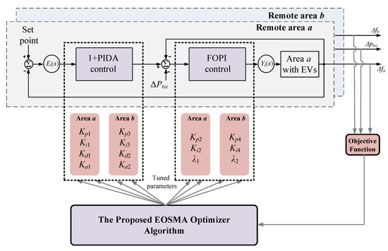
Figure 5.
EOSMA based proposed parameters optimization process.
4.2. EOSMA Optimizer
The EOSMA represents a hybrid optimization technique [73], which is based on two powerful optimization algorithms, the EO optimizer [74] and SMA optimizer [75]. In these, an anisotropic search of SMA is guided by EO’s concentrations update operator to enhance searching efficiency. Afterwards, convergence characteristics are accelerated through updating individual in addition to global optimum by using a greedy strategy. Finally, random operators representing difference mutation are added to EOSMA optimizer to avoid probable local minimums. The update of location in EOSMA is expressed as the following [73]
where denotes that the variable represents a vector quantity, stands for randomly-selected solution in equilibrium pool, denotes to searching agents’ location, represents best found location, and stand for two random vectors representing location and they are selected from individual historical optimum, z = 0.5 stands for setting parameter obtained through hybrid algorithm experiments.
For avoiding local minimum and improving EOSMA exploration ability, searching agents execute random difference mutations scheme after the update in (42). Mutation operator can be mathematically modelled as [73]
where represents random number between [0.3, 0.6]; , , and stand for random-integer vectors with elements between [1, N]; and N stands for population size. After updating the location of the search agent, the EOSMA solution check that the inside range is as follows [73]:
From (44), EOSMA pulls solution vectors beyond searching range back within boundaries. Therefore, invalid searches can be easily produced. Following each fitness function evaluation, an update of individual historic optimum location is made through a greedy strategy, such as the following [73]:
The EOSMA flowchart is clarified in Figure 6 for optimizing LFC parameters.
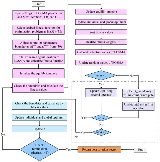
Figure 6.
EOSMA optimization flowchart representation.
5. Results Band Discussions
The Matlab Simulink/m-file environment are used in this paper for simulating interconnected remote MG areas and for designing optimum control parameters. The EOSMA and fitness functions evaluations are programmed using an m-file environment. Maximum iteration number for the evaluated optimizers is unified at 100 iterations with a population size of 8 for all the studied optimizers. The m-file is linked with Simulink model for tuning desired LFC scheme parameters. The PID, PIDA, 1+PIDA, and 1+PID/FOPI are implemented for comparisons purpose with the proposed 3DoF 1+PIDA/FOPI LFC scheme.
Firstly, convergence performance of EOSMA is compared with the EO, SMA, MPA, PSO, and MRFO optimizers at ISE and ITSE in Figure 7, and with IAE and ITAE in Figure 8. For fitness function minimization behavior, the proposed EOSMA based optimization procedure has the lowest value at all the studied functions of ISE, ITSE, IAE, and ITAE. For convergence speed, the EOSMA optimizer converges after 9, 15, 38, and 26 iterations at ISE, ITSE, IAE, and ITAE, respectively. It can be observed the high speed for convergence of the proposed EOSMA method. Moreover, it is clear that the EOSMA optimizer does not fall in the local minimum due to employing the random differential mutation strategy compared with EO and SMA optimizers. The optimum parameters for all studied LFC schemes based on EOSMA optimizer are tabulated in Table 2 at step load case and Table 3 for RESs’ changes case.
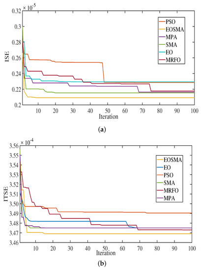
Figure 7.
(a) ISE and (b) ITSE convergence curves comparisons.
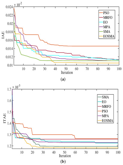
Figure 8.
(a) IAE and (b) ITAE convergence curves comparisons.
Table 2.
The EOSMA-based optimized LFC parameters with step load case.
Table 3.
The EOSMA-based optimized LFC parameters with RESs change case.
The obtained results are organized in six different scenarios to cover all the expected remote MGs disturbances as following:
- Scenario No. 1: The impacts of step loading perturbations (SLP).
- Scenario No. 2: The impacts of SLP and load shedding effects.
- Scenario No. 3: The impacts of ramp loading conditions.
- Scenario No. 4: The impacts of SLP jointly with PV connection/disconnection conditions.
- Scenario No. 5: The impact of high RESs penetrations and low inertia conditions.
- Scenario No. 6: The impacts of severe multiple RESs connections/disconnections.
5.1. Scenario No. 1: Impacts of SLPs
During this scenario, a 1% SLP is made in area a at the starting time at 0 s. Figure 9 shows the waveforms of , , and in this scenario. The proposed 3DoF 1+PIDA/FOPI achieves the lowest peak overshoot/undershoot in operating frequencies of both areas, in addition to the tie-line power. The PID has the worst response, regarding transient peaks and response time. Table 4 tabulates the measured frequency deviations maximum overshoot (MO), maximum undershoot (MU), and settling time (ST) values. The proposed 3DoF 1+PIDA/FOPI has of 0.0002 compared with 0.0024, 0.0022, 0.0015, and 0.0011 p.u. with the studied PID, PIDA, 1+PIDA, and 1+PID/FOPI LFC schemes, respectively. Thence, the proposed 1+PIDA/FOPI LFC scheme possesses the minimum values of in this scenario. Additionally, ST of proposed 1+PIDA/FOPI is 5 s. compared with 18, 14, 12, and 10 with studied PID, PIDA, 1+PIDA, and 1+PID/FOPI LFC schemes, respectively.
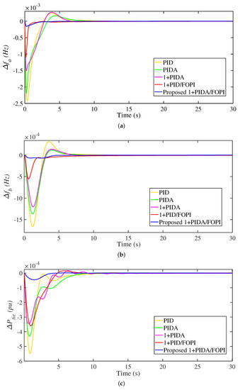
Figure 9.
Frequency and power responses of Scenario 1. (a) ; (b) ; (c) .
Table 4.
Performance measurements for the tested scenarios.
5.2. Scenario No. 2: Impacts of SLPs and Load Shedding Effects
In this scenario, a 5% load increase at 0 s, and 5% reduction in load in area a at 20 s. The results of this case are shown in Figure 10. The 3Dof 1+PIDA/FOPI LFC improves the MGs response at both load changes compared with the high MO/MU/ST with the other compared LFC schemes. For instance, the PID LFC scheme shows the highest MU of at 0 s. of 0.00038 p.u. with the longest ST of 14 s. Whereas the PIDA, 1+PIDA, and 1+PIDA/FOPI achieve PU of of 0.00043 p.u. with ST of 12 s, 0.00042 p.u. with ST of 10 s, and 0.00036 p.u. with ST of 9 s, respectively. From the other side, the proposed 3DoF 1+PIDA/FOPI LFC has the smallest PU of at 0 s of 0.00005 p.u. with the longest ST of 4 s. Therefore, better transient response is obtained through applying the proposed optimum LFC scheme compared with the studied PID, PIDA, 1+PIDA, and 1+PID/FOPI LFC schemes. The recorded results in Table 4 show that the best performance metrics are achieved using the proposed LFC scheme at increase/decrease in loading in both of , , and .
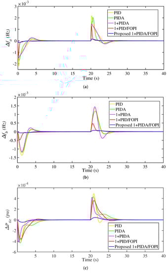
Figure 10.
Frequency and power responses of Scenario 2. (a) ; (b) ; (c) .
5.3. Scenario No. 3: Impacts of Ramp Loading
During this scenario, the loading profile shown in Figure 11 is introduced in area a. The ramp load profile is applied in this scenario to emulate the load characteristics. The MGs response at this scenario is shown in Figure 12 for the waveforms of , , and . It can be shown that the superior performance of the proposed 3Dof 1+PIDA/FOPI LFC for the whole operating scenario. For instance, a measurement of the system response is recorded in Table 4 at the load step at 100 s. The obtained MU in are 0.0148, 0.0095, 0.0041, 0.0174, and 0.0025 at PIDA, 1+PIDA, 1+PIDA/FOPI, and the proposed 3Dof 1+PIDA/FOPI LFC, respectively. Their corresponding ST are 13, 16, 20, 18, and 10 s, respectively. It can be seen that the lowest MU and the shortest ST are obtained using the proposed 3Dof 1+PIDA/FOPI. Whereas the worst response is obtained with the PID, regarding its MU and ST values.
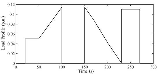
Figure 11.
Loading profile for Scenario 3.
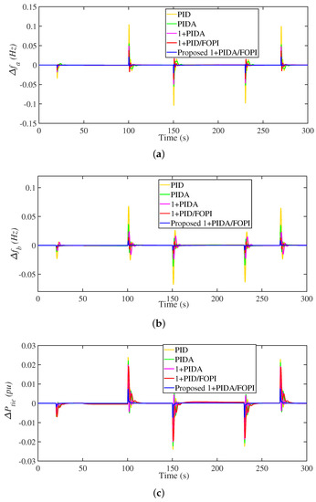
Figure 12.
Frequency and power responses of Scenario 3. (a) ; (b) ; and (c) .
5.4. Scenario No. 4: Impacts of SLP PV Connection/Disconnection
In this scenario, there was a 6% load increase at 0 s, as well as a PV plant connection at 20 s and disconnection at 60 s. The corresponding results of this case are shown in Figure 13. The importance of this scenario is its representation of expected joint SLP and PV connection/disconnection of remote MG systems. IT can be seen that the proposed EOSMA-based optimized 3Dof 1+PIDA/FOPI LFC scheme preserves the MG system response and stability at the three disturbances of this scenario. The employment of two cascaded loops enables the proposed 3Dof 1+PIDA/FOPI LFC scheme to mitigate various existing low- and high-frequency fluctuations compared with the single loop LFC schemes. The PID controller has the worst response in the three disturbances. It can be seen also the effectiveness of the accelerated term in the proposed 3Dof 1+PIDA/FOPI LFC scheme compared with the 1+PID/FOPI LFC scheme. The accelerated term helps at improving system response and reducing waveforms overshoots.
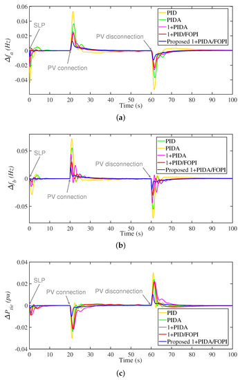
Figure 13.
Frequency and power responses of Scenario 4. (a) ; (b) ; and (c) .
5.5. Scenario No. 5: Impacts of High RESs Penetrations
In this scenario, the system is tested against transients and fluctuated output power from RESs. In which the PV connection is made at 0 s, whereas wind plant connection is made at 40 s. In addition, the dependency of outputted power from RESs on various climatic factors, such as wind speed, temperature, and solar irradiance, has been taken in consideration in this scenario. The PV and winds fluctuations are represented using the implemented models and the corresponding RESs generation profiles are shown in Figure 14. The obtained results of , , and are shown in Figure 15. The obtained MO in , according to the PV connection at 0 s, are 0.1439, 0.1111, 0.0881, 0.0622, and 0.0281 using PIDA, 1+PIDA, 1+PIDA/FOPI, and the proposed 3Dof 1+PIDA/FOPI LFC, respectively. While the corresponding ST response in this scenario are 29, 26, 27, 23, and 13, respectively. This, in turn, confirms the fast and stable response of the proposed 3Dof 1+PIDA/FOPI LFC with considering the RESs characteristics and variations.
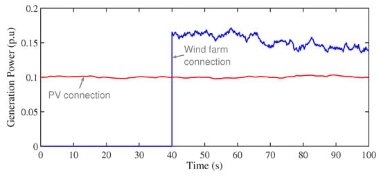
Figure 14.
Loading profile for Scenario 5.
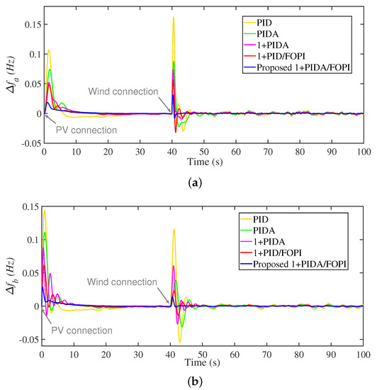
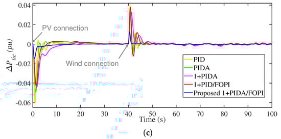
Figure 15.
Frequency and power responses of Scenario 5. (a) ; (b) ; and (c) .
5.6. Scenario No. 6: Impacts of Severe Inertia Condition
During this scenario, severe RESs variations and, hence, inertia conditions are made through adding more RESs in both areas and making disturbances of connection/disconnection of connected renewables. Figure 16 shows the generation power profiles in both areas for this scenario. The obtained , , and waveforms are shown in Figure 17. The measured MGs’ response in Table 4 shows that MO values in with wind plant connection in area a at 40 s are 0.0666, 0.0343, 0.0327, 0.0248, and 0.0074 with PIDA, 1+PIDA, 1+PIDA/FOPI, and the proposed 3Dof 1+PIDA/FOPI LFC, respectively. Whereas the MO values in in this case are 0.0146, 0.0135, 0.0126, 0.0121, and 0.0024, respectively. Additionally, the proposed 3Dof 1+PIDA/FOPI LFC scheme has the better performance with all the RESs connections in this scenario. Thanks to the improved design optimization using EOSMA of the proposed 3Dof 1+PIDA/FOPI LFC, jointly with the proposed controller characteristics, the stability and robustness of remote MG areas are enhanced and improved with considering the high RESs penetration levels and control of plug-in EVs in MG systems.
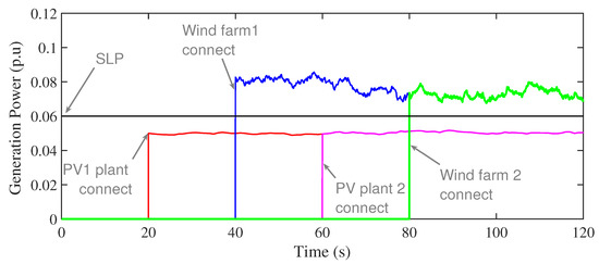
Figure 16.
Loading profile for Scenario 6.
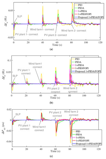
Figure 17.
Frequency and power responses of Scenario 6. (a) ; (b) ; and (c) .
6. Conclusions
A new non-integer LFC scheme has been proposed in this paper based on the 3DoF 1+PIDA cascaded with FOPI controller for LFC in interconnected remote MG systems. The proposed controller benefits the advantages of the PIDA controller with the extra added accelerated term. It is responsible for reducing overshoot/undershoot values and settling time of power systems. Moreover, the cascaded two loops enables faster and better disturbance rejection due to the employment of fast inner frequency loop. The employment of FOPI control in this loop adds more freedom due to the non-integer fractional order operator. Moreover, a new application of the EOSMA optimizer is proposed in this paper for the simultaneous optimization of control parameters. The studied two-area remote MG system is tested under various RESs penetration and scenarios, in addition to various loading behaviors and the contribution of plug-in EVs in the frequency regulation function.
Author Contributions
Conceptualization, M.A., E.A.M. and E.M.A.; Methodology, M.A., A.M.N., E.A.M., F.F.M.E.-S. and M.W.; Software, E.A.M., M.A., E.M.A., A.M.N. and F.F.M.E.-S.; Validation, M.A., E.A.M. and A.M.N.; Formal analysis, E.M.A., E.A.M., A.M.N. and M.A.; Investigation, M.A., E.M.A., F.F.M.E.-S., A.M.N. and E.A.M.; Resources, E.M.A., A.M.N., M.W., and F.F.M.E.-S.; Data curation, M.A., E.A.M., E.M.A., A.M.N. and M.W.; Writing—original draft preparation, M.A., E.A.M., E.M.A., and A.M.N.; Writing—review and editing, M.A., E.M.A., F.F.M.E.-S., and M.W.; Visualization, E.A.M. and E.M.A.; Supervision, F.F.M.E.-S., E.M.A. and M.W.; Funding acquisition, M.A., E.A.M., and M.W. All authors have read and agreed to the published version of the manuscript.
Funding
This study is supported via funding from Prince sattam bin Abdulaziz University project number (PSAU/2023/R/1444). This work was partially supported by JSPS KAKENHI Grant Number JP21K04025. Additionally, the work was supported in part by FONDECYT Iniciación 11230430.
Institutional Review Board Statement
Not applicable.
Informed Consent Statement
Not applicable.
Data Availability Statement
Not applicable.
Conflicts of Interest
The authors declare no conflict of interest.
References
- Shen, X.; Li, X.; Yuan, J.; Jin, Y. A hydrogen-based zero-carbon microgrid demonstration in renewable-rich remote areas: System design and economic feasibility. Appl. Energy 2022, 326, 120039. [Google Scholar] [CrossRef]
- Meena, N.K.; Yang, J.; Zacharis, E. Optimisation framework for the design and operation of open-market urban and remote community microgrids. Appl. Energy 2019, 252, 113399. [Google Scholar] [CrossRef]
- Abolpour, R.; Torabi, K.; Dehghani, M.; Vafamand, N.; Javadi, M.S.; Wang, F.; Catalão, J.P.S. Direct Search Algorithm for Load Frequency Control of a Time-Delayed Electric Vehicle Aggregator. IEEE Trans. Ind. Appl. 2023, 59, 2603–2614. [Google Scholar] [CrossRef]
- Salama, H.S.; Said, S.M.; Aly, M.; Vokony, I.; Hartmann, B. Studying Impacts of Electric Vehicle Functionalities in Wind Energy-Powered Utility Grids With Energy Storage Device. IEEE Access 2021, 9, 45754–45769. [Google Scholar] [CrossRef]
- Oshnoei, A.; Kheradmandi, M.; Blaabjerg, F.; Hatziargyriou, N.D.; Muyeen, S.; Anvari-Moghaddam, A. Coordinated control scheme for provision of frequency regulation service by virtual power plants. Appl. Energy 2022, 325, 119734. [Google Scholar] [CrossRef]
- Li, J.; Yu, T.; Zhang, X. Coordinated load frequency control of multi-area integrated energy system using multi-agent deep reinforcement learning. Appl. Energy 2022, 306, 117900. [Google Scholar] [CrossRef]
- Jia, H.; Li, X.; Mu, Y.; Xu, C.; Jiang, Y.; Yu, X.; Wu, J.; Dong, C. Coordinated control for EV aggregators and power plants in frequency regulation considering time-varying delays. Appl. Energy 2018, 210, 1363–1376. [Google Scholar] [CrossRef]
- Pan, C.; Liaw, C. An adaptive controller for power system load-frequency control. IEEE Trans. Power Syst. 1989, 4, 122–128. [Google Scholar] [CrossRef]
- Oshnoei, A.; Kheradmandi, M.; Khezri, R.; Mahmoudi, A. Robust Model Predictive Control of Gate-Controlled Series Capacitor for LFC of Power Systems. IEEE Trans. Ind. Inform. 2021, 17, 4766–4776. [Google Scholar] [CrossRef]
- Lv, X.; Sun, Y.; Wang, Y.; Dinavahi, V. Adaptive Event-Triggered Load Frequency Control of Multi-Area Power Systems Under Networked Environment via Sliding Mode Control. IEEE Access 2020, 8, 86585–86594. [Google Scholar] [CrossRef]
- Vrdoljak, K.; Perić, N.; Petrović, I. Sliding mode based load-frequency control in power systems. Electr. Power Syst. Res. 2010, 80, 514–527. [Google Scholar] [CrossRef]
- Yu, X.; Tomsovic, K. Application of linear matrix inequalities for load frequency control with communication delays. IEEE Trans. Power Syst. 2004, 19, 1508–1515. [Google Scholar] [CrossRef]
- Rakhshani, E.; Rodriguez, P.; Cantarellas, A.M.; Remon, D. Analysis of derivative control based virtual inertia in multi-area high-voltage direct current interconnected power systems. IET Gener. Transm. Distrib. 2016, 10, 1458–1469. [Google Scholar] [CrossRef]
- Kerdphol, T.; Rahman, F.S.; Mitani, Y.; Watanabe, M.; Kufeoglu, S. Robust Virtual Inertia Control of an Islanded Microgrid Considering High Penetration of Renewable Energy. IEEE Access 2018, 6, 625–636. [Google Scholar] [CrossRef]
- Bu, X.; Yu, W.; Cui, L.; Hou, Z.; Chen, Z. Event-Triggered Data-Driven Load Frequency Control for Multiarea Power Systems. IEEE Trans. Ind. Inform. 2022, 18, 5982–5991. [Google Scholar] [CrossRef]
- Kocaarslan, İ.; Çam, E. Fuzzy logic controller in interconnected electrical power systems for load-frequency control. Int. J. Electr. Power Energy Syst. 2005, 27, 542–549. [Google Scholar] [CrossRef]
- Shiroei, M.; Ranjbar, A. Supervisory predictive control of power system load frequency control. Int. J. Electr. Power Energy Syst. 2014, 61, 70–80. [Google Scholar] [CrossRef]
- Fernández-Guillamón, A.; Gómez-Lázaro, E.; Muljadi, E.; Molina-García, Á. Power systems with high renewable energy sources: A review of inertia and frequency control strategies over time. Renew. Sustain. Energy Rev. 2019, 115, 109369. [Google Scholar] [CrossRef]
- Pandey, S.K.; Mohanty, S.R.; Kishor, N. A literature survey on load–frequency control for conventional and distribution generation power systems. Renew. Sustain. Energy Rev. 2013, 25, 318–334. [Google Scholar] [CrossRef]
- Shankar, R.; Pradhan, S.; Chatterjee, K.; Mandal, R. A comprehensive state of the art literature survey on LFC mechanism for power system. Renew. Sustain. Energy Rev. 2017, 76, 1185–1207. [Google Scholar] [CrossRef]
- Yousri, D.; Babu, T.S.; Fathy, A. Recent methodology based Harris Hawks optimizer for designing load frequency control incorporated in multi-interconnected renewable energy plants. Sustain. Energy Grids Netw. 2020, 22, 100352. [Google Scholar] [CrossRef]
- Dahab, Y.A.; Abubakr, H.; Mohamed, T.H. Adaptive Load Frequency Control of Power Systems Using Electro-Search Optimization Supported by the Balloon Effect. IEEE Access 2020, 8, 7408–7422. [Google Scholar] [CrossRef]
- El Yakine Kouba, N.; Menaa, M.; Hasni, M.; Boudour, M. Optimal load frequency control based on artificial bee colony optimization applied to single, two and multi-area interconnected power systems. In Proceedings of the 2015 3rd International Conference on Control, Engineering & Information Technology (CEIT), Tlemcen, Algeria, 25–27 May 2015; pp. 1–6. [Google Scholar] [CrossRef]
- Ewais, A.M.; Elnoby, A.M.; Mohamed, T.H.; Mahmoud, M.M.; Qudaih, Y.; Hassan, A.M. Adaptive frequency control in smart microgrid using controlled loads supported by real-time implementation. PLoS ONE 2023, 18, e0283561. [Google Scholar] [CrossRef] [PubMed]
- Shabani, H.; Vahidi, B.; Ebrahimpour, M. A robust PID controller based on imperialist competitive algorithm for load-frequency control of power systems. ISA Trans. 2013, 52, 88–95. [Google Scholar] [CrossRef]
- Youssef, A.R.; Mallah, M.; Ali, A.; Shaaban, M.F.; Mohamed, E.E.M. Enhancement of Microgrid Frequency Stability Based on the Combined Power-to-Hydrogen-to-Power Technology under High Penetration Renewable Units. Energies 2023, 16, 3377. [Google Scholar] [CrossRef]
- Abid, S.; El-Rifaie, A.M.; Elshahed, M.; Ginidi, A.R.; Shaheen, A.M.; Moustafa, G.; Tolba, M.A. Development of Slime Mold Optimizer with Application for Tuning Cascaded PD-PI Controller to Enhance Frequency Stability in Power Systems. Mathematics 2023, 11, 1796. [Google Scholar] [CrossRef]
- Zhang, G.; Daraz, A.; Khan, I.A.; Basit, A.; Khan, M.I.; Ullah, M. Driver Training Based Optimized Fractional Order PI-PDF Controller for Frequency Stabilization of Diverse Hybrid Power System. Fractal Fract. 2023, 7, 315. [Google Scholar] [CrossRef]
- Shiva, C.; Shankar, G.; Mukherjee, V. Automatic generation control of power system using a novel quasi-oppositional harmony search algorithm. Int. J. Electr. Power Energy Syst. 2015, 73, 787–804. [Google Scholar] [CrossRef]
- Mohanty, B.; Panda, S.; Hota, P.K. Controller parameters tuning of differential evolution algorithm and its application to load frequency control of multi-source power system. Int. J. Electr. Power Energy Syst. 2014, 54, 77–85. [Google Scholar] [CrossRef]
- Sahu, R.; Panda, S.; Rout, U.K.; Sahoo, D. Teaching learning based optimization algorithm for automatic generation control of power system using 2-DOF PID controller. Int. J. Electr. Power Energy Syst. 2016, 77, 287–301. [Google Scholar] [CrossRef]
- Dash, P.; Saikia, L.; Sinha, N. Automatic generation control of multi area thermal system using Bat algorithm optimized PD–PID cascade controller. Int. J. Electr. Power Energy Syst. 2015, 68, 364–372. [Google Scholar] [CrossRef]
- Raju, M.; Saikia, L.; Sinha, N. Automatic generation control of a multi-area system using ant lion optimizer algorithm based PID plus second order derivative controller. Int. J. Electr. Power Energy Syst. 2016, 80, 52–63. [Google Scholar] [CrossRef]
- Latif, A.; Hussain, S.M.S.; Das, D.C.; Ustun, T.S. Optimization of Two-Stage IPD-(1I) Controllers for Frequency Regulation of Sustainable Energy Based Hybrid Microgrid Network. Electronics 2021, 10, 919. [Google Scholar] [CrossRef]
- Gheisarnejad, M. An effective hybrid harmony search and cuckoo optimization algorithm based fuzzy PID controller for load frequency control. Appl. Soft Comput. 2018, 65, 121–138. [Google Scholar] [CrossRef]
- Prakash, S.; Sinha, S. Simulation based neuro-fuzzy hybrid intelligent PI control approach in four-area load frequency control of interconnected power system. Appl. Soft Comput. 2014, 23, 152–164. [Google Scholar] [CrossRef]
- Latif, A.; Paul, M.; Das, D.C.; Hussain, S.M.S.; Ustun, T.S. Price Based Demand Response for Optimal Frequency Stabilization in ORC Solar Thermal Based Isolated Hybrid Microgrid under Salp Swarm Technique. Electronics 2020, 9, 2209. [Google Scholar] [CrossRef]
- Hussain, I.; Das, D.C.; Latif, A.; Sinha, N.; Hussain, S.S.; Ustun, T.S. Active power control of autonomous hybrid power system using two degree of freedom PID controller. Energy Rep. 2022, 8, 973–981. [Google Scholar] [CrossRef]
- Parmar, K.S.; Majhi, S.; Kothari, D. Load frequency control of a realistic power system with multi-source power generation. Int. J. Electr. Power Energy Syst. 2012, 42, 426–433. [Google Scholar] [CrossRef]
- Bakeer, A.; Magdy, G.; Chub, A.; Jurado, F.; Rihan, M. Optimal Ultra-Local Model Control Integrated with Load Frequency Control of Renewable Energy Sources Based Microgrids. Energies 2022, 15, 9177. [Google Scholar] [CrossRef]
- Yakout, A.H.; AboRas, K.M.; Kotb, H.; Alharbi, M.; Shouran, M.; Samad, B.A. A Novel Ultra Local Based-Fuzzy PIDF Controller for Frequency Regulation of a Hybrid Microgrid System with High Renewable Energy Penetration and Storage Devices. Processes 2023, 11, 1093. [Google Scholar] [CrossRef]
- Zaid, S.A.; Bakeer, A.; Magdy, G.; Albalawi, H.; Kassem, A.M.; El-Shimy, M.E.; AbdelMeguid, H.; Manqarah, B. A New Intelligent Fractional-Order Load Frequency Control for Interconnected Modern Power Systems with Virtual Inertia Control. Fractal Fract. 2023, 7, 62. [Google Scholar] [CrossRef]
- Jung, S.; Dorf, R. Analytic PIDA controller design technique for a third order system. In Proceedings of the35th IEEE Conference on Decision and Control, Kobe, Japan, 13 December 1996; Volume 3, pp. 2513–2518. [Google Scholar] [CrossRef]
- Kumar, M.; Hote, Y.V. Maximum sensitivity-constrained coefficient diagram method-based PIDA controller design: Application for load frequency control of an isolated microgrid. Electr. Eng. 2021, 103, 2415–2429. [Google Scholar] [CrossRef]
- Yakout, A.H.; Attia, M.A.; Kotb, H. Marine Predator Algorithm based Cascaded PIDA Load Frequency Controller for Electric Power Systems with Wave Energy Conversion Systems. Alex. Eng. J. 2021, 60, 4213–4222. [Google Scholar] [CrossRef]
- Elsaied, M.M.; Attia, M.A.; Mostafa, M.A.; Mekhamer, S.F. Application of Different Optimization Techniques to Load Frequency Control with WECS in a Multi-Area System. Electr. Power Compon. Syst. 2018, 46, 739–756. [Google Scholar] [CrossRef]
- Kumar, M. Resilient PIDA Control Design Based Frequency Regulation of Interconnected Time-Delayed Microgrid Under Cyber-Attacks. IEEE Trans. Ind. Appl. 2023, 59, 492–502. [Google Scholar] [CrossRef]
- Ayas, M.S.; Sahin, E. FOPID controller with fractional filter for an automatic voltage regulator. Comput. Electr. Eng. 2021, 90, 106895. [Google Scholar] [CrossRef]
- Fathy, A.; Alharbi, A.G. Recent Approach Based Movable Damped Wave Algorithm for Designing Fractional-Order PID Load Frequency Control Installed in Multi-Interconnected Plants With Renewable Energy. IEEE Access 2021, 9, 71072–71089. [Google Scholar] [CrossRef]
- Singh, K.; Amir, M.; Ahmad, F.; Refaat, S.S. Enhancement of Frequency Control for Stand-Alone Multi-Microgrids. IEEE Access 2021, 9, 79128–79142. [Google Scholar] [CrossRef]
- Peddakapu, K.; Mohamed, M.; Srinivasarao, P.; Leung, P. Simultaneous controllers for stabilizing the frequency changes in deregulated power system using moth flame optimization. Sustain. Energy Technol. Assess. 2022, 51, 101916. [Google Scholar] [CrossRef]
- Singh, K. Load frequency regulation by de-loaded tidal turbine power plant units using fractional fuzzy based PID droop controller. Appl. Soft Comput. 2020, 92, 106338. [Google Scholar] [CrossRef]
- Oshnoei, S.; Aghamohammadi, M.; Oshnoei, S.; Oshnoei, A.; Mohammadi-Ivatloo, B. Provision of Frequency Stability of an Islanded Microgrid Using a Novel Virtual Inertia Control and a Fractional Order Cascade Controller. Energies 2021, 14, 4152. [Google Scholar] [CrossRef]
- Oshnoei, S.; Oshnoei, A.; Mosallanejad, A.; Haghjoo, F. Contribution of GCSC to regulate the frequency in multi-area power systems considering time delays: A new control outline based on fractional order controllers. Int. J. Electr. Power Energy Syst. 2020, 123, 106197. [Google Scholar] [CrossRef]
- Peddakapu, K.; Srinivasarao, P.; Mohamed, M.; Arya, Y.; Kishore, D.K. Stabilization of frequency in Multi-Microgrid system using barnacle mating Optimizer-based cascade controllers. Sustain. Energy Technol. Assess. 2022, 54, 102823. [Google Scholar] [CrossRef]
- Arya, Y.; Kumar, N.; Dahiya, P.; Sharma, G.; Çelik, E.; Dhundhara, S.; Sharma, M. Cascade-IλDμN controller design for AGC of thermal and hydro-thermal power systems integrated with renewable energy sources. IET Renew. Power Gener. 2021, 15, 504–520. [Google Scholar] [CrossRef]
- Malik, S.; Suhag, S. A Novel SSA Tuned PI-TDF Control Scheme for Mitigation of Frequency Excursions in Hybrid Power System. Smart Sci. 2020, 8, 202–218. [Google Scholar] [CrossRef]
- Sahu, R.K.; Panda, S.; Biswal, A.; Sekhar, G.C. Design and analysis of tilt integral derivative controller with filter for load frequency control of multi-area interconnected power systems. ISA Trans. 2016, 61, 251–264. [Google Scholar] [CrossRef] [PubMed]
- Priyadarshani, S.; Subhashini, K.R.; Satapathy, J.K. Pathfinder algorithm optimized fractional order tilt-integral-derivative (FOTID) controller for automatic generation control of multi-source power system. Microsyst. Technol. 2021, 27, 23–35. [Google Scholar] [CrossRef]
- Oshnoei, A.; Khezri, R.; Muyeen, S.M.; Oshnoei, S.; Blaabjerg, F. Automatic Generation Control Incorporating Electric Vehicles. Electr. Power Compon. Syst. 2019, 47, 720–732. [Google Scholar] [CrossRef]
- Singh, K.; Amir, M.; Ahmad, F.; Khan, M.A. An Integral Tilt Derivative Control Strategy for Frequency Control in Multimicrogrid System. IEEE Syst. J. 2021, 15, 1477–1488. [Google Scholar] [CrossRef]
- Ahmed, E.M.; Mohamed, E.A.; Elmelegi, A.; Aly, M.; Elbaksawi, O. Optimum Modified Fractional Order Controller for Future Electric Vehicles and Renewable Energy-Based Interconnected Power Systems. IEEE Access 2021, 9, 29993–30010. [Google Scholar] [CrossRef]
- Mohamed, E.A.; Ahmed, E.M.; Elmelegi, A.; Aly, M.; Elbaksawi, O.; Mohamed, A.A.A. An Optimized Hybrid Fractional Order Controller for Frequency Regulation in Multi-Area Power Systems. IEEE Access 2020, 8, 213899–213915. [Google Scholar] [CrossRef]
- Ahmed, E.M.; Elmelegi, A.; Shawky, A.; Aly, M.; Alhosaini, W.; Mohamed, E.A. Frequency Regulation of Electric Vehicle-Penetrated Power System Using MPA-Tuned New Combined Fractional Order Controllers. IEEE Access 2021, 9, 107548–107565. [Google Scholar] [CrossRef]
- Latif, A.; Hussain, S.M.S.; Das, D.C.; Ustun, T.S. Optimum Synthesis of a BOA Optimized Novel Dual-Stage PI − (1 + ID) Controller for Frequency Response of a Microgrid. Energies 2020, 13, 3446. [Google Scholar] [CrossRef]
- Sulaiman, M.H.; Mustaffa, Z.; Saari, M.M.; Daniyal, H. Barnacles Mating Optimizer: A new bio-inspired algorithm for solving engineering optimization problems. Eng. Appl. Artif. Intell. 2020, 87, 103330. [Google Scholar] [CrossRef]
- Arya, Y. A novel CFFOPI-FOPID controller for AGC performance enhancement of single and multi-area electric power systems. ISA Trans. 2020, 100, 126–135. [Google Scholar] [CrossRef]
- Arya, Y. A new optimized fuzzy FOPI-FOPD controller for automatic generation control of electric power systems. J. Frankl. Inst. 2019, 356, 5611–5629. [Google Scholar] [CrossRef]
- Gheisarnejad, M.; Khooban, M.H. Design an optimal fuzzy fractional proportional integral derivative controller with derivative filter for load frequency control in power systems. Trans. Inst. Meas. Control. 2019, 41, 2563–2581. [Google Scholar] [CrossRef]
- Arya, Y. Improvement in automatic generation control of two-area electric power systems via a new fuzzy aided optimal PIDN-FOI controller. ISA Trans. 2018, 80, 475–490. [Google Scholar] [CrossRef]
- Khamies, M.; Magdy, G.; Selim, A.; Kamel, S. An improved Rao algorithm for frequency stability enhancement of nonlinear power system interconnected by AC/DC links with high renewables penetration. Neural Comput. Appl. 2021, 34, 2883–2911. [Google Scholar] [CrossRef]
- Elkasem, A.H.A.; Kamel, S.; Hassan, M.H.; Khamies, M.; Ahmed, E.M. An Eagle Strategy Arithmetic Optimization Algorithm for Frequency Stability Enhancement Considering High Renewable Power Penetration and Time-Varying Load. Mathematics 2022, 10, 854. [Google Scholar] [CrossRef]
- Yin, S.; Luo, Q.; Zhou, G.; Zhou, Y.; Zhu, B. An equilibrium optimizer slime mould algorithm for inverse kinematics of the 7-DOF robotic manipulator. Sci. Rep. 2022, 12, 9421. [Google Scholar] [CrossRef] [PubMed]
- Faramarzi, A.; Heidarinejad, M.; Stephens, B.; Mirjalili, S. Equilibrium optimizer: A novel optimization algorithm. Knowl.-Based Syst. 2020, 191, 105190. [Google Scholar] [CrossRef]
- Li, S.; Chen, H.; Wang, M.; Heidari, A.A.; Mirjalili, S. Slime mould algorithm: A new method for stochastic optimization. Future Gener. Comput. Syst. 2020, 111, 300–323. [Google Scholar] [CrossRef]
- Falahati, S.; Taher, S.A.; Shahidehpour, M. A new smart charging method for EVs for frequency control of smart grid. Int. J. Electr. Power Energy Syst. 2016, 83, 458–469. [Google Scholar] [CrossRef]
- Khokhar, B.; Dahiya, S.; Parmar, K.P.S. A Robust Cascade Controller for Load Frequency Control of a Standalone Microgrid Incorporating Electric Vehicles. Electr. Power Compon. Syst. 2020, 48, 711–726. [Google Scholar] [CrossRef]
- Ray, P.K.; Mohanty, S.R.; Kishor, N. Proportional–integral controller based small-signal analysis of hybrid distributed generation systems. Energy Convers. Manag. 2011, 52, 1943–1954. [Google Scholar] [CrossRef]
- Das, D.C.; Roy, A.; Sinha, N. GA based frequency controller for solar thermal–diesel–wind hybrid energy generation/energy storage system. Int. J. Electr. Power Energy Syst. 2012, 43, 262–279. [Google Scholar] [CrossRef]
- Markova, E.; Sidler, I.; Solodusha, S. Integral Models Based on Volterra Equations with Prehistory and Their Applications in Energy. Mathematics 2021, 9, 1127. [Google Scholar] [CrossRef]
- Muftahov, I.; Sidorov, D.; Zhukov, A.; Panasetsky, D.; Foley, A.; Li, Y.; Tynda, A. Application of Volterra Equations to Solve Unit Commitment Problem of Optimised Energy Storage and Generation. arXiv 2016, arXiv:1608.05221. [Google Scholar] [CrossRef]
- Muftahov, I.; Sidorov, D.; Zhukov, A.; Karamov, D. Volterra Model of Energy Storage with Nonlinear Efficiency in Integrated Power Systems. In Advances in Intelligent Systems and Computing; Springer International Publishing: Berlin/Heidelberg, Germany, 2021; pp. 808–815. [Google Scholar] [CrossRef]
- Markova, E.V.; Sidorov, D.N. On one integral Volterra model of developing dynamical systems. Autom. Remote Control 2014, 75, 413–421. [Google Scholar] [CrossRef]
- Falahati, S.; Taher, S.A.; Shahidehpour, M. Grid Secondary Frequency Control by Optimized Fuzzy Control of Electric Vehicles. IEEE Trans. Smart Grid 2018, 9, 5613–5621. [Google Scholar] [CrossRef]
- Luo, X.; Xia, S.; Chan, K.W. A decentralized charging control strategy for plug-in electric vehicles to mitigate wind farm intermittency and enhance frequency regulation. J. Power Sources 2014, 248, 604–614. [Google Scholar] [CrossRef]
- Ota, Y.; Taniguchi, H.; Nakajima, T.; Liyanage, K.M.; Baba, J.; Yokoyama, A. Autonomous Distributed V2G (Vehicle-to-Grid) Satisfying Scheduled Charging. IEEE Trans. Smart Grid 2012, 3, 559–564. [Google Scholar] [CrossRef]
- Abraham, R.J.; Das, D.; Patra, A. Automatic generation control of an interconnected hydrothermal power system considering superconducting magnetic energy storage. Int. J. Electr. Power Energy Syst. 2007, 29, 571–579. [Google Scholar] [CrossRef]
- Micev, M.; Ćalasan, M.; Oliva, D. Fractional Order PID Controller Design for an AVR System Using Chaotic Yellow Saddle Goatfish Algorithm. Mathematics 2020, 8, 1182. [Google Scholar] [CrossRef]
- Dulf, E.H. Simplified Fractional Order Controller Design Algorithm. Mathematics 2019, 7, 1166. [Google Scholar] [CrossRef]
- Motorga, R.; Mureșan, V.; Ungureșan, M.L.; Abrudean, M.; Vălean, H.; Clitan, I. Artificial Intelligence in Fractional-Order Systems Approximation with High Performances: Application in Modelling of an Isotopic Separation Process. Mathematics 2022, 10, 1459. [Google Scholar] [CrossRef]
Disclaimer/Publisher’s Note: The statements, opinions and data contained in all publications are solely those of the individual author(s) and contributor(s) and not of MDPI and/or the editor(s). MDPI and/or the editor(s) disclaim responsibility for any injury to people or property resulting from any ideas, methods, instructions or products referred to in the content. |
© 2023 by the authors. Licensee MDPI, Basel, Switzerland. This article is an open access article distributed under the terms and conditions of the Creative Commons Attribution (CC BY) license (https://creativecommons.org/licenses/by/4.0/).