1. Introduction
Eating is an essential part of everyone’s life. However, older adults may have difficulty eating or swallowing because of sarcopenia, declining cognitive functions, tissue elasticity, and neuromuscular control of the neck [
1,
2], or other health conditions such as strokes, age-related neurological conditions, and gastroesophageal reflux [
3,
4]. Dysphagia, classified as a sign or symptom, is defined as the difficulty in swallowing [
5], in which foods/liquids may obstruct the passage towards the stomach [
6]. Individuals with dysphagia may have problems with drinking, eating, controlling saliva, and taking medications. A quarter of the adult population manifested swallowing problems, while the prevalence of dysphagia in stroke, institutionalized dementia, and Parkinson’s patients was 41%, 45%, and 60%, respectively [
2,
7,
8].
Complications of dysphagia are major causes of mortality and morbidity in the elderly and include aspiration pneumonia, malnutrition, and dehydration [
9]. Dysphagic individuals reported a mortality rate that was 1.7 times higher and spent approximately USD 6000 more in hospitalization expenses compared to the non-dysphagic group [
1]. Moreover, the fear and anxiety of choking also severely impacted their quality of life and psychological wellbeing [
10]. Over one-third of dysphagic older adults avoid eating because of their conditions [
11]. In fact, up to 68% of dysphagic elderly people lived in nursing homes, and about one-third of them lived independently [
12], which inherited a significant burden and risk to the healthcare system and society.
Screening or assessment is crucial to prompting immediate management and rehabilitative interventions to reduce complication risks. Clinically, fiber-optic endoscopic evaluation of swallowing (FEES) and the video-fluoroscopy swallowing study (VFSS) are standard methods for dysphagia screening [
13]. The procedure of FEES involves passing the endoscopic instrument through the nose to observe the pharynx and larynx when the individual is swallowing saliva with and without food consistencies [
13]. Similarly, VFSS evaluates the swallowing function with different food consistencies, but through fluoroscopy over the oral cavity, pharynx, and cervical esophagus [
13]. There are some drawbacks to these two methods. FEES induces pain and discomfort, while topical anesthesia may be applied sometimes. The VFSS exposes patients to radiation hazards and contrast agents [
13]. Moreover, FEES and the VFSS are expensive and require professionals to operate.
It is demanding to develop alternative bedside methods that are valid and reliable [
14]. Non-instrumental bedside assessments relied heavily on experts or therapists to conduct anamnesis, morphodynamical, and gustative function evaluations [
15], whereas other related tests, such as the 3-ounce water swallowing test [
16] and cough reflex test [
17], lacked sensitivity and predictive strength [
18] despite being routinely carried out in nursing homes or care homes. The use of acoustic and accelerometric sensors has been one of the common approaches to analyze swallowing [
19,
20]. The accelerometer is positioned on the surface of the skin above the larynx, where muscle movements take place when an individual swallows [
21]. On the other hand, through a microphone near the throat, the chewing and swallowing sounds could be collected and analyzed to determine the food consistencies and viscosities and thus the swallowing conditions. Hidden Markov or other deep learning models were used for signal processing and analysis [
22,
23,
24]. However, the approach was subject to background noise and may require additional pre-processing and segmentation of the acoustic data [
25]. For the piezoelectric sensors, they were in the form of necklaces or patches that were versatile and light. The sensors detected physical strain and movement, which were subsequently processed with deep learning models to recognize chewing and swallowing motions [
26,
27,
28]. It might also be challenging to implement contact-based sensors for older adults, especially those with dementia [
29].
Recently, noncontact optical-based approaches using infrared depth cameras have emerged and been adopted for different mobile health applications [
30,
31,
32,
33]. Specific to dysphagia, An et al. [
34] developed a liquid viscosity estimation model using the built-in camera of the smartphone with a convolutional neural network (CNN). Some other researchers also attempted to estimate the swallowing time using a depth camera [
35]. Another study focused on measuring laryngeal movement via depth images, modeled by a decision tree [
36]. We believed that the infrared depth camera could analyze the swallowing movement of the throat and compromise privacy. With the advancement of deep learning models in computer vision, we anticipated that they could help identify swallowing and thus abnormalities of swallowing. While CNN was a class of models commonly used for image classification, recent studies demonstrated that another cutting-edge class of models, Transformers, which lay upon the core of natural language processing (NLP) [
37], could effectively model the spatiotemporal relationship of image data (i.e., video data) and thus improve the classification performance.
On the other hand, regardless of the kind of model, an activation function is often required after the linear transformation of each layer. It is essential to provide nonlinearity in order to facilitate the learning of complicated input–output interactions [
38]. In more technical terms, activation functions turn the weighed sum of inputs into an output value and transmit it to the nodes of the next layer. During model training, the choice of activation function is often determined by compromising convergence, complexity, smooth gradient flow, and data preservation during model training [
38]. A Rectified Linear Unit (ReLU) is one of the common activation functions utilized by renowned networks, including AlexNet, GoogleNet, ResNet, and MobileNets. Other more recent activation functions, such as Swish, Exponential Linear Unit (ELU), Gaussian Error Linear Unit (GELU), and Gated Linear Units (GLU) have garnered attention for being superior to ReLU in certain tasks, despite the fact that the majority of model developments still adhere to the well-established ReLU [
39]. Contemporary CNN networks often incorporate residual blocks with a Rectified Linear Unit (ReLU) as the default activation function. Nevertheless, the developers of ResNet and their successors did not justify or evaluate the choice of activation functions.
To this end, the objective of this study was to evaluate the performance of deep learning models (CNNs and Transformers) in classifying swallowing events from infrared depth camera video data. For the model with the best performance, we would then analyze the activation function that may further enhance the performance. The goal was to select the appropriate model and activation functions for this application at the outset and to facilitate a full-scale study for deployment in the future. This work represented the initial step to pave the road towards affordable and accessible instrumented dysphagia screening.
2. Materials and Methods
2.1. Participant Recruitment
We recruited 65 healthy adults (28 males and 37 females) from the university campus. Inclusion criteria were adults with no prior swallowing deprivation or disorder and no operation history for the head or neck within three months. Exclusion criteria were adults with difficulties in communication due to consciousness disturbance and patients with a tracheotomy hole. The participants had a mean age of 43.2 years (SD: 17.7, range: 18 to 77), an average height of 164.6 cm (SD: 8.19 cm, range: 148 cm to 183 cm), and a weight of 62.9 kg (SD: 13.5 kg, range: 40 kg to 100 kg). The experiment was approved by the Institutional Review Board of the university (reference No.: HSEARS20210416005). Prior to the start of the experiment, all participants were provided with oral and written descriptions of the experimental procedures, and they signed an informed consent form indicating their understanding and agreement to participate.
2.2. System Setup
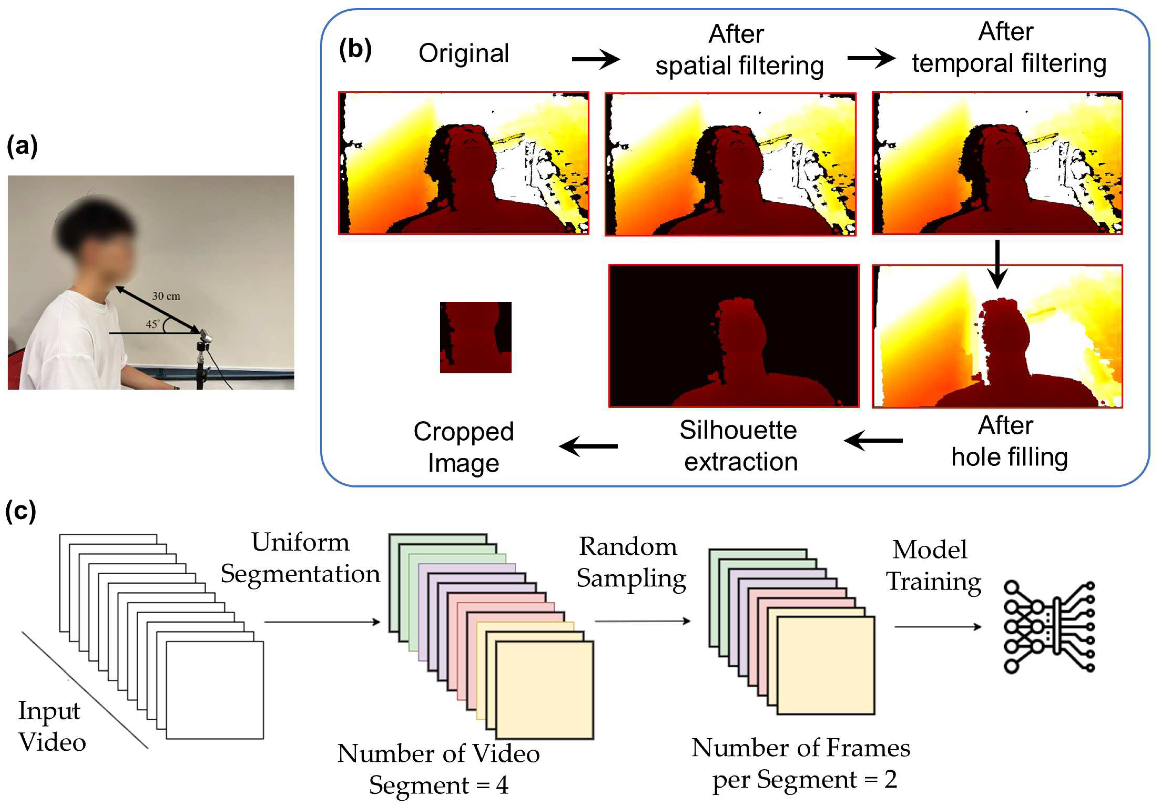
An infrared Red-Blue-Green (RGB) stereo-based depth camera (Realsense D435i, Intel Corp., Santa Clara, CA, USA) was positioned to capture the entire swallowing process using the RealSense viewer program. Some preliminary tests were previously carried out and it was determined that the camera should be oriented at a 45° angle from the horizontal plane and placed 30 cm away from the neck of the participant (
Figure 1a) to acquire the lower face and neck regions. The depth image data were captured at a resolution of 640 × 480 pixels, a frame rate of 30 frames per second, and a pixel depth of 2 bytes per pixel (or 1 mm per depth unit). The data were transmitted and processed on a personal computer.
2.3. Experimental Procedure
During the experiment, we recorded the lower face and neck (lip, mandible, and throat) motions for both non-swallowing and swallowing tasks. For the non-swallowing tasks, participants were asked to pronounce vowels, “/eɪ/”, “/iː/”, “/aɪ/”, “/oʊ/”, “/u:/” (i.e., /a/, /e/, /i/, /o/, /u/), in addition to performing a deep breath. After completing the non-swallowing motion tests, participants were asked to perform swallowing tasks. The first swallowing task was to eat (swallow) a cracker, approximately 45 mm × 45 mm in size. The second task was to drink (swallow) a cup of 10 mL of water. Participants were asked to consume as much as possible while taking bites/boluses at their comfortable size/volume.
The recording time depended on the actual duration of the tasks for each participant and trial. The swallowing time was approximately 1.0 to 1.5 s. Similarly, all tasks were repeated four times. Therefore, there was a total of 520 and 1560 sample data for all participants on the swallowing and non-swallowing tasks, respectively. The full dataset, with both swallowing and non-swallowing tasks, constituted 2080 sample data. The actual swallowing or non-swallowing tasks performed by the participants (i.e., ground truth) were manually labeled on each clip.
2.4. Data Processing
The overall data processing framework was shown in
Figure 1b, which consisted of frame-by-frame filtering and video sampling. After data collection, we processed the data to improve the image (frame) quality and reduce noise. We followed the processing pipeline using RealSense SDK, as recommended by the official documents. For each frame, we first transformed the depth domain of the images to the disparity domain. Next, we applied spatial and temporal filters to denoise. The spatial filter was a one-dimensional edge-preserving spatial filter using a high-order domain transformation [
41]. It aimed to smooth the depth noise while preserving the edges. The temporal filter was similar to the spatial filter but suppressed artifacts across consecutive frames of the depth video sequence. The strength of smoothing was controlled by the parameters
α and
δ, for calculating the one-dimensional exponential moving average (EMA). It is defined by the recursive Equation (1):
where coefficient
refers to the degree of weighting decrease,
represents the latest recorded value for disparity or depth, and
is the value of the EMA at a previous time period, denoted as
t.
When α is set to 1, no filtering is applied, while an α of zero results in an infinite history for the filtering. Additionally, the delta threshold () was introduced. If the difference in depth values between neighboring pixels exceeds , α would be temporarily reset to one, which disables the filtering. In other words, if an edge is detected, the smoothing function is temporarily turned off. However, this may result in artifacts, depending on the direction of the edge traversed (i.e., right-to-left or left-to-right). To mitigate this, two bi-directional passes would be employed in both the vertical and horizontal directions of the images.
In temporal filtering, the same EMA smoothing was employed in the time domain. Similar to the spatial filter, was used to represent the extent of the temporal history that should be averaged. The advantage of this approach is that it allows fractional frames to be effectively averaged. By setting , there would be no filtering, while = 0 would increase the averaging effect and result in a smoother output, allowing fine-grained smoothing beyond simple discrete frame averaging. Moreover, it is also important to incorporate the delta threshold, , to reduce the temporal smoothing effects near edges and ensure that missing depth information is not included in the averaging. We applied RealSense SDK default values for and , where and for the spatial filter, and and for the temporal filter. Since image reconstruction of the stereo depth camera is based on a triangulation technique, the noise would appear at a level correlated with the squared rate of the camera–subject distance. In this context, and would need to be adjusted based on the camera–subject distance, such that over-smoothing of near-range data and under-smoothing of far-range data could be avoided. We adopted a simpler approach by transforming the data into disparity domains before applying the filter.
After the filtering process, the images (frames) were back-transformed to the depth domain. We applied the hole-filling filter (boundary fill from Realsense SDK) to gaps or missing regions in depth maps that might result from occlusions and reflections. Subsequently, we removed the image background by zeroing the data with depth values larger than 60 cm and segmenting the silhouette of the subject. The region of interest (ROI) was located by first identifying the centroid of the silhouette
based on the image moment, the weighted averages of the image pixels’ values, which are defined in Equations (2) and (3).
where
i and
j constitute the order of the moment, and
I(
x,
y) represents the pixel value of row
x and column
y. The first-order moments
and
normalized by the zero-order moment
would yield the centroid of the silhouette
and crop out a 224 × 224 pixel region from (
− 112,
− 168) to (
+ 112,
+ 56).
This setting was assigned based on our pilot analysis to ensure that the throat, mandibular (jaw), and lip regions were covered. To avoid excessive memory and computational requirements associated with utilizing the entire sequence of video frames in training, frames were sampled from the video using the temporal segment network [
40]. As shown in
Figure 1c, depth video frames were sampled by dividing the entire footage into several snippets, followed by a random selection of frames from each snippet. In our case, we decided to divide the depth videos into four snippets and randomly sample two frames from each snippet, as determined by our pilot analysis. The approach could ensure that every part of the video was representative of the loaded frames, and the method would be flexible enough to accommodate arbitrary and varying video lengths [
40]. The pseudocode of the process is illustrated in
Algorithm A1.
2.5. Activation Functions
While ReLU was the default activation function for X3D, Slowfast, and R(2+1)D, GELU was utilized by ViViT and TimeSFormer. In this study, we tested five activation functions, including ReLU [
42], LeakyReLU [
43], GELU [
44], ELU [
45], a Sigmoid-weighted Linear Unit (SiLU) [
46], and a Gated Linear Unit (GLU) [
47], on the model with the best performance. For the best-performing activation function, we would further conduct hyperparameter tuning of the activation function. The formulations with an input to a neuron (
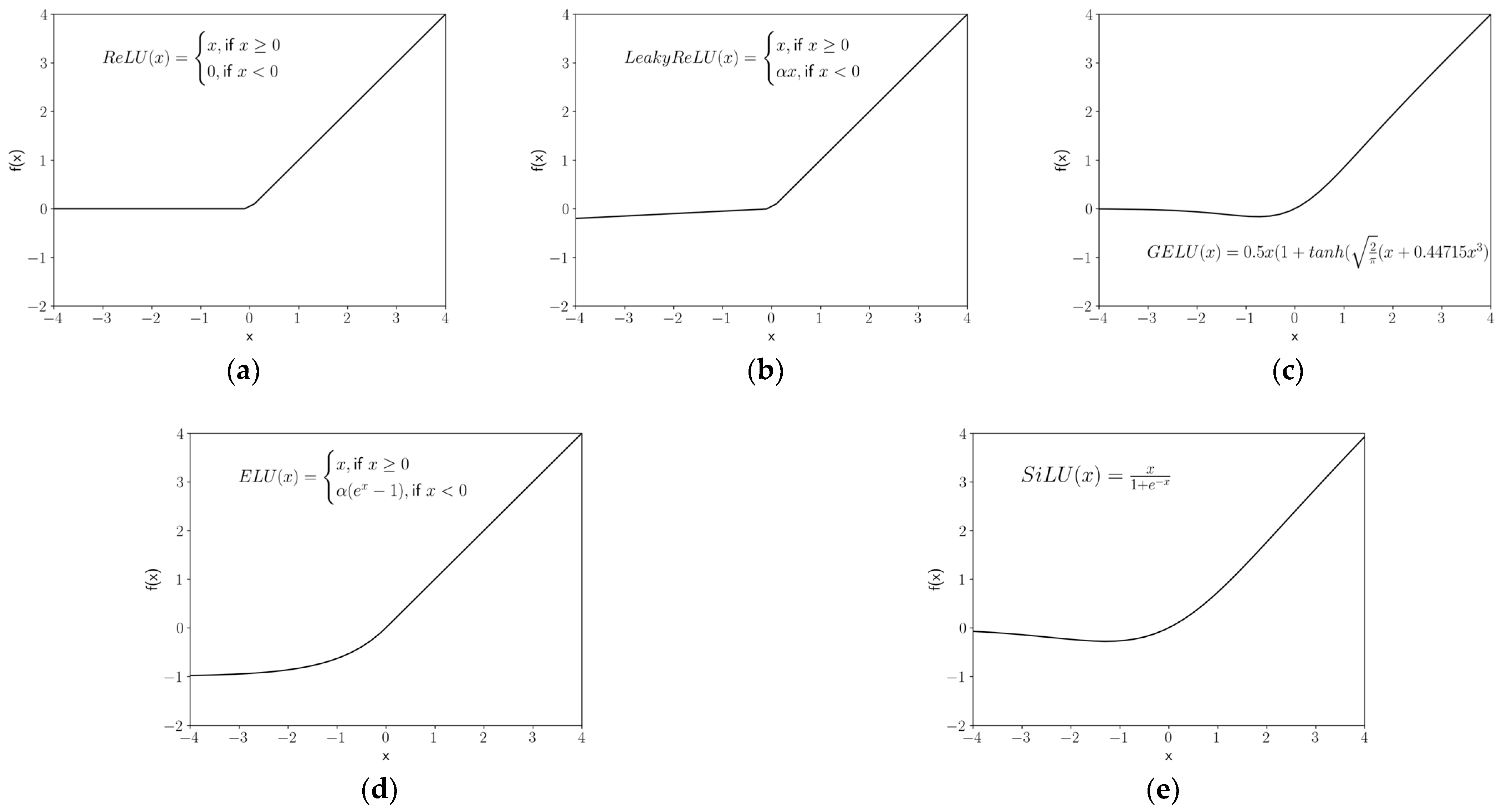
x) for all activation functions are illustrated in Equations (4)–(9) and compared in
Figure 2.
ReLU is a piecewise linear function that outputs the input directly if it is positive, and zero if it is negative, which is the default for most of networks due to its simplicity and high performance.
LeakyReLU (a particular kind of Parametric ReLU) is based on ReLU but returns a small negative value or slope (default
α = 0.01) if the input is negative to account for the situation in which a large number of neuron inputs are negatives. Therefore, some information is “leaked” to prevent information loss (dead neurons) [
48]. The ELU adopted a similar strategy but introduced exponential nonlinearity on negative inputs to mitigate the vanishing gradient problem (
α default is one), whilst the SiLU utilized a Sigmoid function (
σ). Vanishing gradient problems appear when lower layers of a network have gradients that are close to zero because higher layers are virtually saturated at −1 or 1 due to the
tanh function [
49].
GELU multiplies the input neuron by a random value from 0 to 1, calculated by the cumulative distribution function of the Gaussian distribution
. When the value of the input neuron is small, there is a large likelihood that the function’s output would be zero (i.e.,
). GeLU is based on the assumption that the input neuron follows a normal distribution, especially after batch normalization.
where
k is the patch size, and
m and
n are the number of input and output feature maps, respectively.
The GLU is constructed by the linear project of the neuron input , multiplied by the Sigmoid gates . The element-wise multiplication of the gates on the input projection matrices could control the information passed on the hierarchy.
2.6. Model Training
Five cutting-edge deep learning models were trained for swallowing/non-swallowing classification, including two models of the Transformer class (TimeSFormer [
50], Video Vision Transformer (ViViT) [
51],) and three models of the CNN class (SlowFast [
52], X3D [
53] and R(2+1)D [
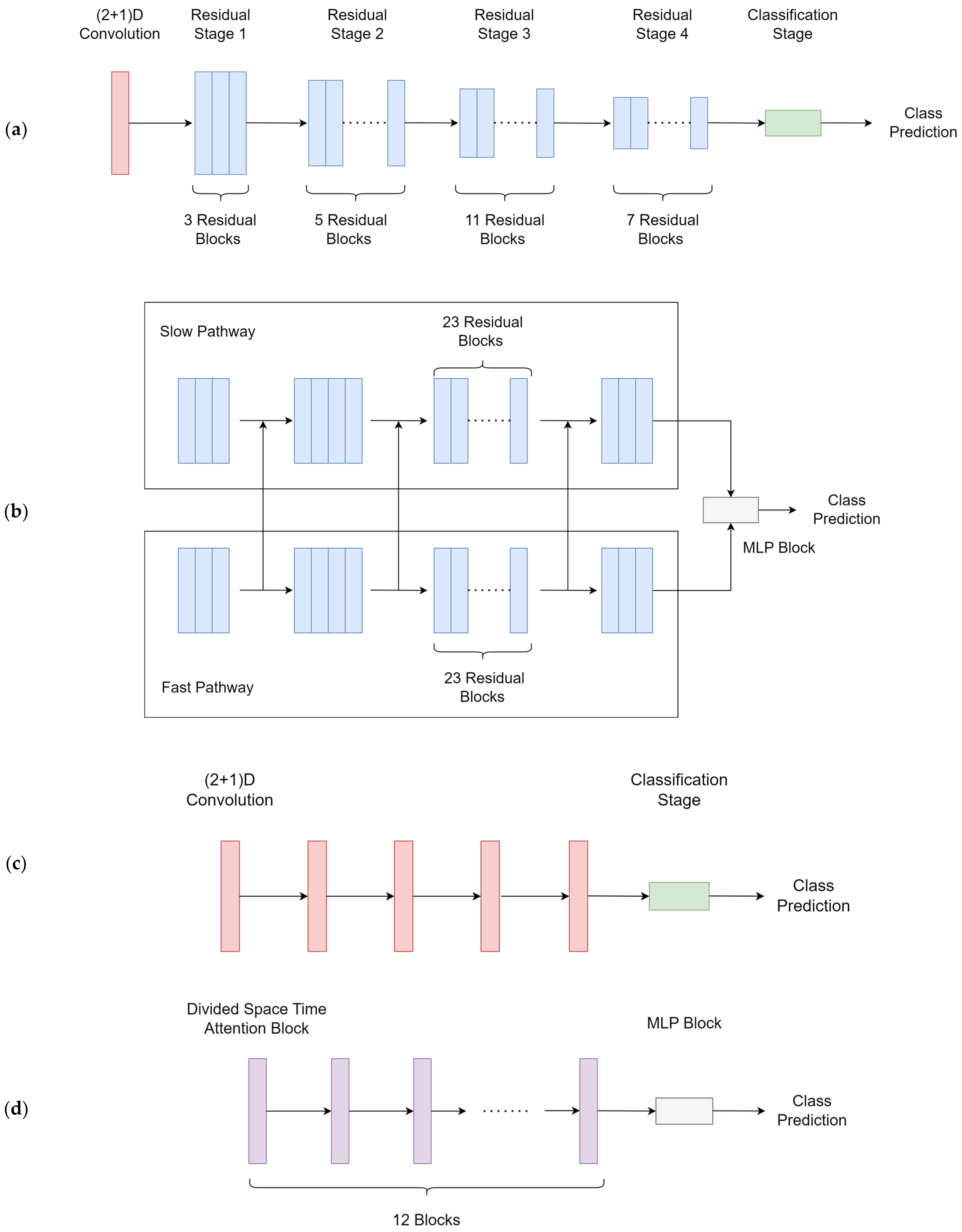
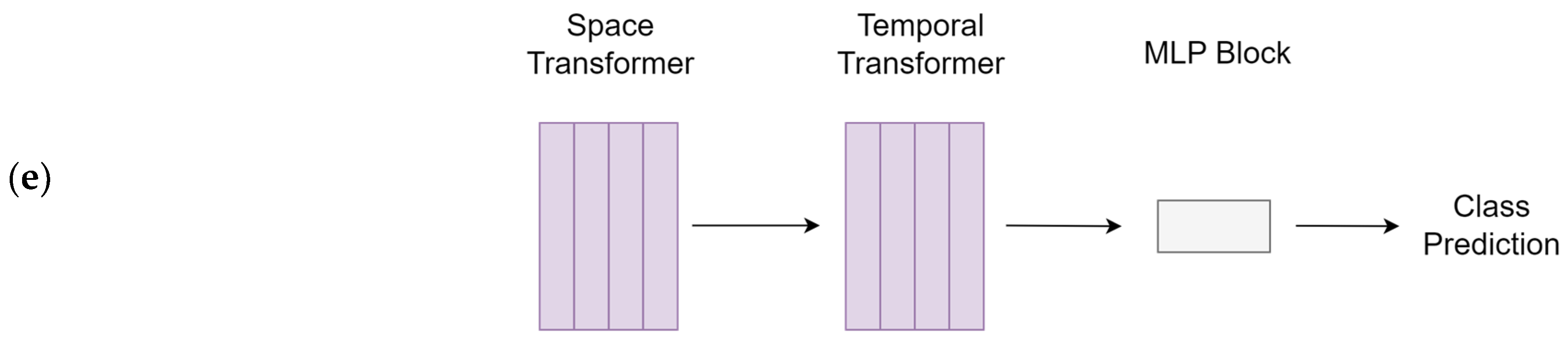
54]). Model architectures are illustrated in
Figure 3. Explanations of the models were provided in the discussion section. The models were trained using a computational unit with Intel Core i7 12700 and Nvidia RTX 4090. The total parameters and training time referenced to our computer are provided in
Table 1.
We split the data into training, validation, and testing datasets at a ratio of 7:2:1. The models were trained using the training datasets. The performance of the model on the validation set during training was monitored to prevent overfitting. We performed 200 training epochs, with early stopping if the best performance did not improve in the next 20 iterations. The Adam optimizer was used for all models at a 0.0001 learning rate using cross entropy as the loss function. The pseudocode for the Adam optimizer is included in
Algorithm A2.
The training batch size was set to four. We performed 100 training epochs, with early stopping if the best validation loss value did not improve in the next 20 iterations. For hyperparameters, TimeSFormer’s attention mechanism was divided into space-time attention, where temporal attention and spatial attention were separately applied one after the other [
50]. The patch size of ViViT was set to eight. The ResNet101 backbone was employed in the SlowFast model. All other unspecified hyperparameters were set to default, corresponding to each of the models. All processes were implemented using the PyTorch library [
55].
2.7. Outcome Measures and Data Analysis (Model Evaluation)
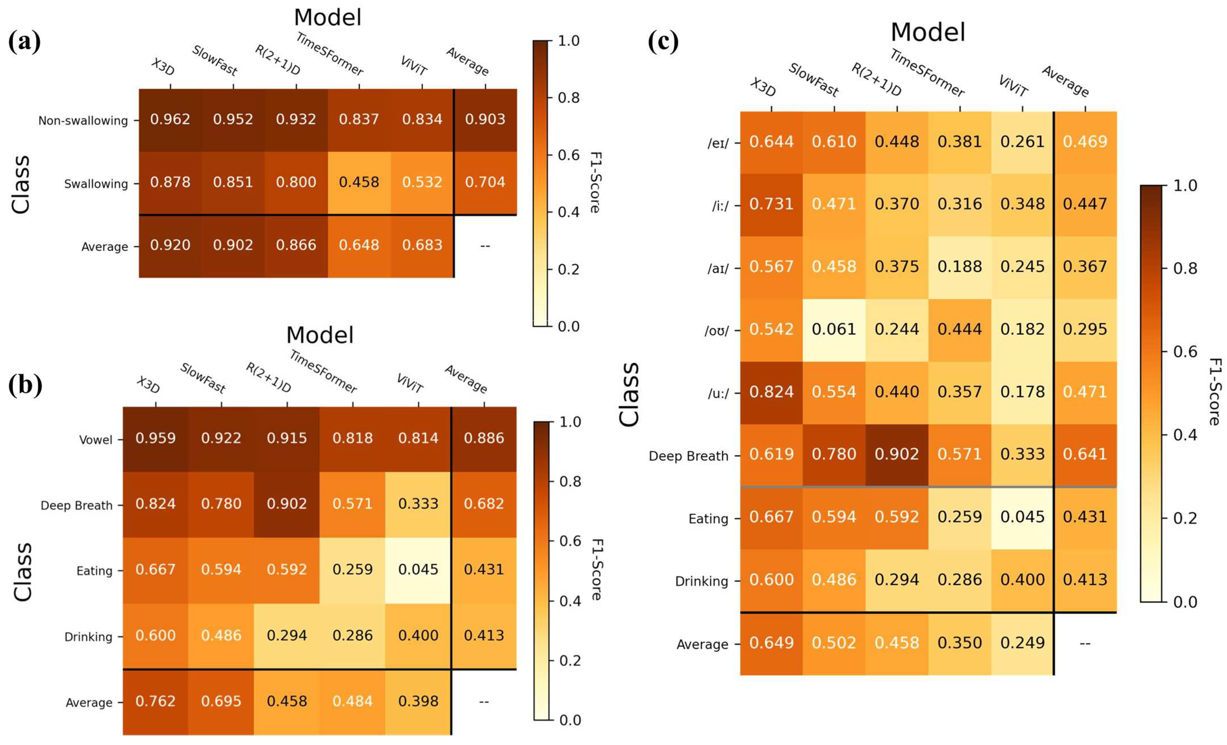
Model evaluation was conducted by making predictions by inputting testing datasets onto the models. The primary analysis involved the overall performance in classifying the swallowing and non-swallowing tasks (i.e., coarse classification). Thereupon, two fine-grained classifications (subgroup analyses) on four classes and eight classes were performed. The former involved vowel pronunciation, deep breathing, eating, and drinking, while the latter involved the eight swallowing and non-swallowing tasks. On the best model, the same analysis would be conducted to compare the performance of various activation functions.
The F1-score was used as the primary outcome, which was believed to be less prone to an imbalanced class bias [
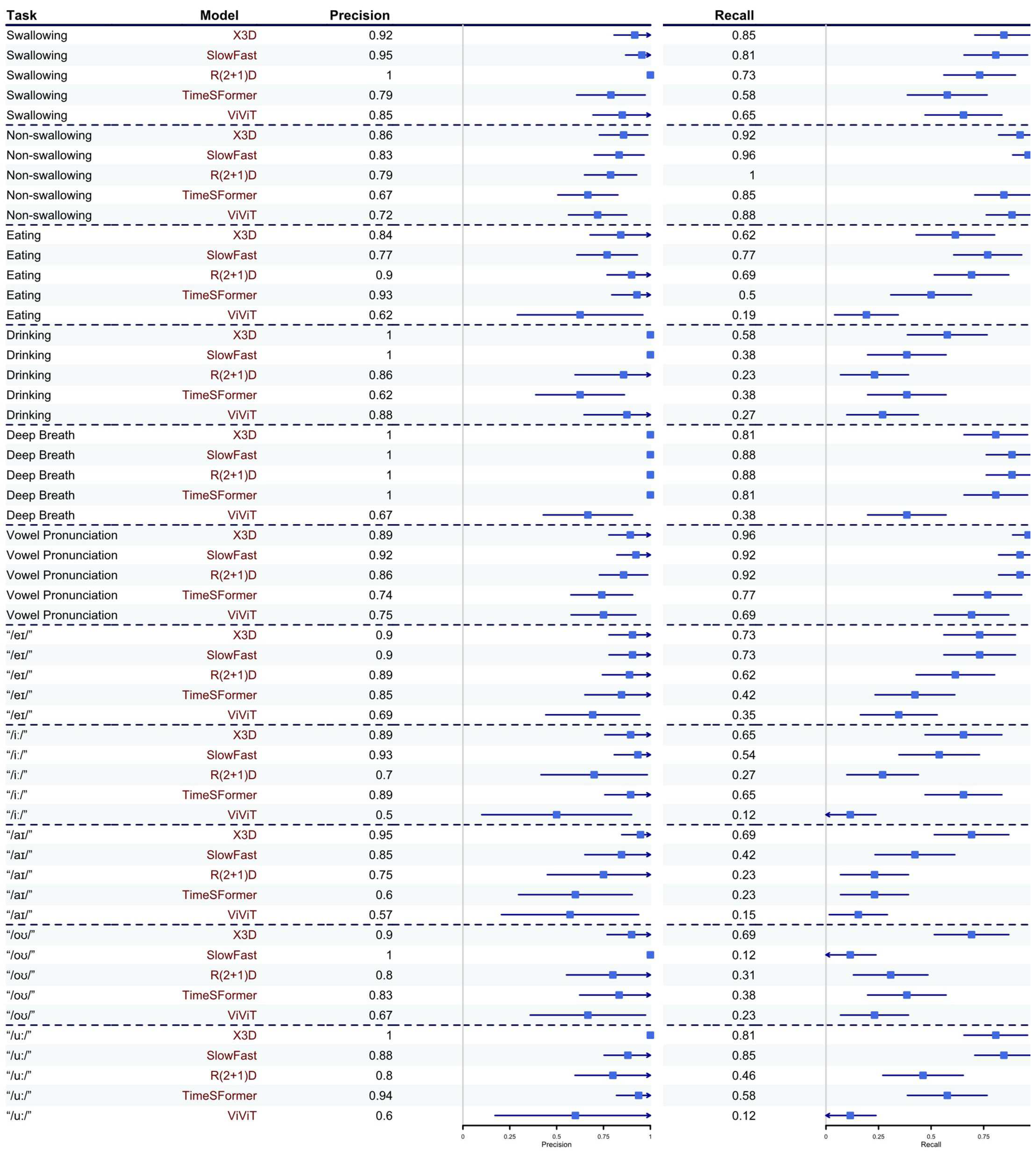
56]. It is the harmonic mean of precision and recall, which is calculated by reciprocating the arithmetic mean of the reciprocals of precision and recall, as shown in Equations (10)–(12). Precision was defined as the proportion of positive predictions that were correct, while recall was the proportion of true positives that were correctly identified [
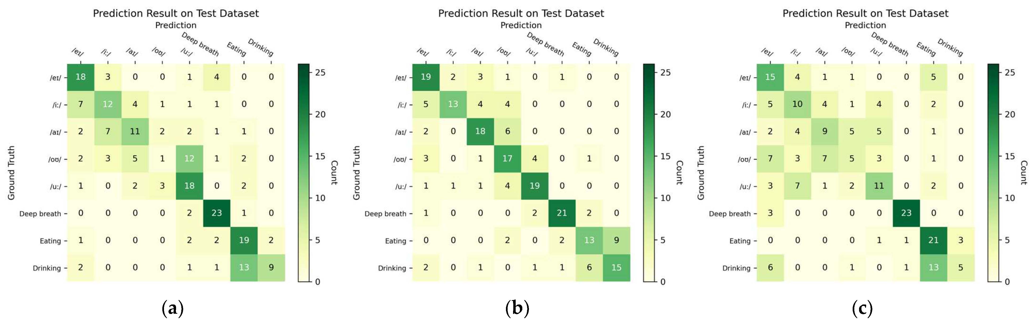
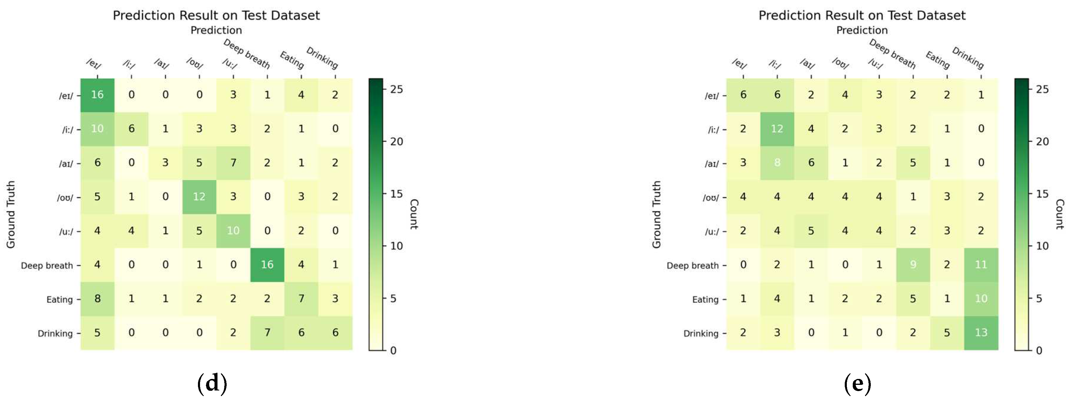
57]. These outcome measures were derived from the confusion matrix (i.e., contingency table) that visualized the relationship between the predicted and actual (ground truth) class labels for the testing dataset. The cells of the table consisted of counts of true positives (TP), true negatives (TN), false positives (FP), and false negatives (FN). The confusion matrix of the best-performing model was presented, in addition to the precision and recall for the other models and subgroup analyses. The counts were also used to analyze the source of the misclassification. Moreover, the Area under the receiver-operating characteristics curve (AUC) was used to evaluate the discrimination power of a binary classifier model. As a rule-of-thumb, we considered an F1-score over 0.70 as acceptable, 0.85 as good, and 0.9 as excellent.
The F1-score was calculated in Equations (10)–(12).
where
Pc is precision and
Rc is recall. TP, FP, and FN are true positive, false positive, and false negative, respectively.
For model evaluation, an adjustment of the F1-score, precision, and recall were supplemented by bootstrapping (
n = 26) on the major class to accommodate the imbalance in class size because of multiclass subgroup analyses (
Algorithm A3). Confidence intervals of precision and recall for bootstrapping were estimated by their standard errors assuming a binomial distribution.
4. Discussion
The novelty of this research lies in the application of depth cameras, in addition to state-of-the-art deep learning techniques including CNNs and Transformer models, to analyze and classify swallowing and non-swallowing tasks, which paves the road towards accessible instrumental dysphagia screening. We believed that this may be one of the first works of its kind. Moreover, the swallow monitoring system could be expanded to evaluate patients with eating behavioral and malnutritional problems and to facilitate biofeedback training [
58,
59].
Five cutting-edge deep learning models were used and compared, including TimeSFormer, ViViT, SlowFast, X3D, and R(2+1)D. These models were specialized in leveraging both spatial and temporal information from video sequences to perform tasks such as action recognition, object detection, and video segmentation, while addressing various challenges unique to video analysis, such as the temporal variability and the need for efficient and scalable architectures. [
60]. The two Transformer models differed from one another in the design of the attention scheme. TimeSformer embedded frame-level patches and learned spatiotemporal features by dividing temporal and spatial attention schemes within each block [
50]. On the other hand, ViViT proposed multiple-head self-attention architectures that accounted for the factorization of spatial and temporal dimensions of the input [
51].
For the CNNs, SlowFast consisted of a slow and a fast pathway processing the same input with different temporal resolutions. The slow pathway was a standard 3D CNN, while the fast pathway integrated a 2D CNN with a temporal down-sampling unit. The two pathways were joined with a Time-strided convolution (T-conv) [
52]. X3D was built using a ResNet structure and the Fast pathway of the SlowFast model, along with degenerated (single frame) temporal input [
53]. Moreover, the characteristics of R(2+1)D were the utilization of a 2D convolutional filter with a 1D temporal convolutional filter, governed by the hyperparameter related to the intermediate subspace between the spatial and temporal convolutions [
54].
X3D was the best model in our study with good-to-excellent performance (F1-score: 0.920; adjusted F1-score: 0.885) in classifying swallowing and non-swallowing conditions despite the fact that the performance was just acceptable. The model focused on one data dimension at a time in building up the model blocks to accommodate the level of complexity, which might be appropriate and efficient for our occasion. For the other two CNNs, R(2+1)D manifested spatiotemporal representation through temporal convolutions, while the SlowFast model captured high-level semantics and spatiotemporal information through the slow and fast pathways. These approaches could be vulnerable to the predefined layer size and number of layers, which might require strategies for extensive hyperparameter optimization to arrest critical spatiotemporal features. The hyperparameter tuning process could be very time-consuming and demanding of computational power because of the higher dimensionality of video data, compared to those working on numeric and image data. On the other hand, our initial hypothesis was that the Transformers could outperform the CNNs because of their long-range capturing capacity and attention mechanism. Nevertheless, Transformers exhibited poor performance in our study because of the small dataset size. In fact, Transformers placed a very high demand on the size of the dataset [
61]. We did not pre-train the Transformers because a large-depth video dataset was not available in the public domain.
The classification of the depth camera relied on manifested morphological motions of the lip (mouth), mandibular (jaw), and neck (throat) regions. Swallowing and non-swallowing could be easier to classify because of the discernible depth of the throat, with and without bolus. Although eating behaviors can be represented by “periodic” mandibular (jaw) activities (i.e., chewing) [
62], our study found it difficult to discriminate between eating and drinking, probably due to their comparable lip and throat motions. Capturing hand movements might help distinguish the type of foods/liquids. On the other hand, while pronunciation could be recognized by lip movements, some vowels had subtle lip apertures and might vary depending on individuals’ speaking habits or speaking countries [
63]. This could be the reason for the low accuracy in the fine-grained classification of vowel pronunciation. Nevertheless, the success in recognizing talking (pronunciation), breathing, and eating/drinking might facilitate monitoring systems for sleep apnea and somniloquy.
Real-time and continuous extraction and identification of high-level spatial and temporal features were the challenges in this study. The experimental protocol itself might confound the data features. In particular, swallowing tasks generally had a shorter duration than non-swallowing tasks. We endeavored to apply the temporal segment network [
40] to equalize the amount of information in the temporal domain to ensure that the model was analyzing the spatiotemporal features of the data instead of the length of the recording. Nevertheless, the approach might not account for the dynamic time wrapping issue [
64]. For example, the variations on the start/stop instants of the recording and features might fail to “synchronize and align” the temporal features corresponding to each task. These would lead to bias during random sampling within the temporal segment network.
The optimal training/validation/testing ratio for machine learning was mostly empirical and lacked precise recommendations [
65,
66]. While Joseph [
65] and Dubbs [
66] suggested that the number of parameters and the size of the dataset could be used to estimate the splitting ratio for linear models and Ridge and Lasso regression, a general law for the splitting ratio, determined analytically or asymptotically for all models, has not yet been established [
66]. A rule of thumb was to divide the data in an 80/20 ratio based on the Pareto principle, while some advised allocating 70% of data for model training and distributing the remaining data evenly for model validation and testing. Reducing the size of the training dataset, especially for small datasets, would increase the variance of the parameter estimates of the model, while the trade-off between the validation and testing datasets was decided by the need to prevent over-fitting [
67]. Guyon [
68] proposed that the training size determines the model inference, while the validation set (or cross-validation) would serve to indicate which family of feature patterns (recognizer) works best. In this study, we adopted a 70/20/10 approach because our dataset was small, and a larger training set ratio was preferred. In fact, an optimal splitting ratio may also depend on the type of models, data dimensionality, and validation methods, such as cross-validation and bootstrapping [
69,
70], posing difficulties for deep learning models with complex model architecture and high data dimensionality, and warranting further investigations on the theories behind hunches.
Activation functions contribute to the advance in deep learning [
71] and have a substantial effect on the behavior and performance of deep learning models [
72,
73,
74]. However, numerous studies overlooked the activation function and associated hyperparameters (e.g., slope coefficient,
α) [
48,
75] and relied on model defaults. In fact, selecting the activation function is exceedingly difficult and typically requires extensive trial-and-error attempts. It depends on the dataset and the problem at hand [
75,
76]. From a different point of view, it is dependent on the input-output relationship of each node and each layer, but it is hard to trace since the neural network may be a direct rich space of ill-posed functions [
77]. The challenge is exacerbated by the notion of the “edge of chaos”, which states the model should neither run in an overly ordered nor overly random state [
78]. Several studies attempted to offer solutions to this issue. Dushkoff and Ptucha [
79] employed more than one activation function depending on the classification error. Jagtap, et al. [
76] integrated a basic activation function, using a gated or hierarchical structure to adapt to the inputs, while Li et al. [
80] utilized a differential evolution algorithm to determine the activation function based on the input data. Through a “smart search” method, Marchisio et al. [
74] realized an automatic selection of the best possible activation functions for each layer. Nevertheless, the optimization of activation functions and associated hyperparameters requires considerable computing power and time.
Imbalanced classes were one of the challenges in different fields using machine learning/deep learning, including medical imaging [
81,
82], digital health [
83,
84,
85], and machine learning-driven instruments [
19,
86]. In fact, imbalanced class scenarios often skew towards the negative cases, since disease cases (positives) are generally rarer than non-disease cases (negatives). Models tend to predict “negative” in a highly imbalanced class problem in order to maximize their probability of making a correct “guess” [
87]. In such cases, the loss function of the models could be penalized using a class-weighted inverse proportion of the class size [
88]. Nevertheless, we avoid the imbalanced class problem on the training dataset by collecting the same amount of data for each task. For the multiclass issue in the subgroup analysis [
89], we mitigate the imbalanced class problem in testing with a bootstrapping approach.
There were some limitations in this research. Firstly, the relatively small size of the testing set may restrict the robustness of the model. In our study, a single incorrect prediction of the testing data would deflate the model accuracy by about 0.5%. A k-fold cross-validation could improve the model robustness upon deployment [
90]. Secondly, our protocol design did not purport to cover every swallowing task. While we took reference from the comprehensive assessment protocol for swallowing (CAPS) [
91], identifying the fewest swallowing tasks necessary to accurately depict swallowing functions would be helpful to develop the instrument for dysphagia screening and lessen the time and inconvenience during the assessment, which warrant further investigations. The inclination of the camera was determined based on our pilot experiment that better captured the frontal view of the neck area. We believed that our model would be insensitive to the variations of the camera orientation since the model could accommodate the variations by the affine transformation nature of the convolutional layer. Moreover, with respect to subject recruitment, gender could be a significant confounder and critical feature in the study because of the larger Adam’s apple in males that might need to be input into the model. Secondly, the duration of the data samples (i.e., sample/sequence length) was about 1.0 to 1.5 s. To learn the temporal features effectively and produce accurate predictions, some models, especially Transformers, need sufficient temporal duration for each data sample [
37,
92]. Although the sample length requirement could be task-specific, longer data sequences provide more context for the model to learn complex relationships between inputs and outputs [
37,
92]. Data augmentation techniques might be used to prolong the data sequences [
93]. For example, repeating the short video frames to lengthen the video clip. Moreover, data augmentation could help resolve the demand for large datasets in Transformers. Data augmentation for depth frames could be achieved by adding rotations about the three-dimensional axes to simulate different orientations or viewpoints of the depth camera [
94]. Alternatively, the Synthetic Minority Over-sampling Technique (SMOTE) could be one way to create synthetic samples by interpolating neighboring instances of that class, which could also be used to resolve the imbalanced class problem [
95]. Lastly, we have not constructed explainability maps to understand the attention of the network on salient features and locations since there are no available libraries that could be applied directly to four-dimensional data in our cases, which warrants further investigations.


 ,
, 


