Abstract
This paper introduces a parallel meta-heuristic algorithm called Cuckoo Flower Search (CFS). This algorithm combines the Flower Pollination Algorithm (FPA) and Cuckoo Search (CS) to train Multi-Layer Perceptron (MLP) models. The algorithm is evaluated on standard benchmark problems and its competitiveness is demonstrated against other state-of-the-art algorithms. Multiple datasets are utilized to assess the performance of CFS for MLP training. The experimental results are compared with various algorithms such as Genetic Algorithm (GA), Grey Wolf Optimization (GWO), Particle Swarm Optimization (PSO), Evolutionary Search (ES), Ant Colony Optimization (ACO), and Population-based Incremental Learning (PBIL). Statistical tests are conducted to validate the superiority of the CFS algorithm in finding global optimum solutions. The results indicate that CFS achieves significantly better outcomes with a higher convergence rate when compared to the other algorithms tested. This highlights the effectiveness of CFS in solving MLP optimization problems and its potential as a competitive algorithm in the field.
Keywords:
evolutionary algorithm; neural networks; FNN; multi-layer perceptron; cuckoo flower search MSC:
90C26; 68U05
1. Introduction
Over the past decades, artificial intelligence (AI), and particularly machine learning (ML), has paved the way for researchers to study nature and build problem solving models. In particular, studying the phenomena of natural selection, social behavior, and other patterns has led to the rise of evolutionary computing, swarm intelligence, and neural networks (NN). NN are the most significant invention in the arena of soft computing, inspired by neurons present in human brain. The basic NN model was conceptualized by McCulloch and Pitts [1]. There are various types of NNs, including Kohonen self-organizing networks [2], recurrent NN [3], spiking NN [4], feed-forward networks (FNN) [5], and others. Among these NNs, FNN are the simplest, with low computational cost and high performance. FNN receive input from one side and provides output at the other. The FNN is generally unidirectional, with multiple layers in between. If there is only a single layer, the network is called a Single-layer perceptron (SLP) [6]. SLPs are used for solving linear problems. If there are multiple layers, called a multi-layer perceptron (MLP) [1,7], these networks are used to solve non-linear problems.
All NNs have a common feature of learning from experience. Such NNs are called Artificial NN (ANN), and they adapt themselves according to given set of inputs. ANNs can be supervised using an external source for providing feedback [8,9], or they can be unsupervised [10,11], taking the form of a NN that adapts to its own inputs without any external feedback. Training NNs to achieve the highest possible performance is performed by a trainer. The trainer provides the NN with a set of input samples, modifies it with the structural parameters of the NN, and finally, when the training process is complete, the trainer is omitted and the NN is set as active and is available for use. There are two types of trainers: deterministic and stochastic. Supervised learning to solve problems, brought about with the advent of the Back propagation (BP) algorithm [12] and the gradient search algorithm, are deterministic methods that aim at training through mathematical optimization to achieve maximum performance. These trainers are simple and have higher convergence speed, leading to a global optimum from a single solution. These optimization methods have a problem of becoming in a local optima that is sometimes mistaken as global optima. On the other hand, stochastic training methods use stochastic optimization methods to achieve desired performance. These methods initiate training with a random solution and enhance it to achieve a global optimum. Randomness in stochastic methods provides local optima avoidance but these methods are slower than deterministic methods [13,14]. Stochastic trainers are generally used in literature due to high avoidance of local optimum.
Stochastic trainers can be single-solution or multi-solution. For a single-solution, the NN is constructed by training it with a single random solution and evolving it iteratively until stopping criteria is satisfied. Simulated annealing (SA) [15,16], hill climbing [17], and others [18,19] are examples of single-solution NNs. Multi-solution NNs, on the other hand, are initiated with multiple random solutions and evolve each solution unless the stopping criteria is met. These criteria include Genetic algorithm (GA) [20], Ant colony optimization (ACO) [21], Artificial Bee colony (ABC) [22,23], Particle swarm optimization (PSO) [24,25], Differential evolution (DE) [26], Teacher-learning based optimization (TLBO) [27], Invasive weed algorithm (IWO) [28], ensemble techniques [29], Grey Wolf optimization (GWO) [30], and others. These algorithms have high performance in terms of finding approximate global optimum solutions. This inspires us to develop a new meta-heuristic and apply it efficiently for training NNs.
In this work, a new parallel algorithm based on Cuckoo Search (CS) [31] and Flower Pollination Algorithm (FPA) [32], which we have named Cuckoo Flower Search (CFS), is introduced. The main motivation for this work is the problem of local optima stagnation and premature convergence problems of already existing algorithms. CFS has been tested on standard benchmark functions and compared with state-of-the-art algorithms for establishing its competitiveness. In addition, it has been further tested on FNN-MLP as an application to real world problems. Nineteen benchmark functions have been used to analyze the performance of the proposed algorithm. These benchmark functions consist of unimodal functions, multi-modal functions, and fixed-dimension functions. These problems are highly challenging and any algorithm performing well on these functions is considered to be a good algorithm. A comparison with GWO, CS, FPA, BFP, and others was also conducted. Statistical tests have also been performed to prove the superiority of CFS over other comparable algorithms. The major contributions of the paper are highlighted as:
- To avoid premature convergence and local optima stagnation, best known properties of FPA and CS are added to the proposed algorithm.
- The global and local search phase equations of FPA and CS are optimized for addition in the proposed algorithm.
- Solutions generated by FPA and CS are compared and best among the two is selected as the current best solution. These solutions are further generated over the course of iterations to find the global best solution.
- A greedy selection operation is followed for retaining the best solution over subsequent iterations.
- The proposed algorithm is tested on 19 classical benchmark functions, and Wilcoxon rank-sum test is done to prove the significance of the algorithm statistically.
- Finally, five real-world datasets, including Heart, Breast cancer, Iris, Ballon, and XOR, are optimized using the proposed algorithm.
- The source code of CFS algorithm is available at: https://github.com/rohitsalgotra/CFS (accessed on 20 June 2023).
The rest of the paper is organized as follows: Section 2 describes the preliminary definitions of FNN and MLP. The basics of CS and FPA are detailed in Section 3. Section 4 describes the proposed CFS algorithm. Section 5 presents with the results and discussion. Finally, Section 6 concludes the paper.
2. Feed-Forward Neural Networks and Multi-Layer Perceptron
FNNs are that are unidirectional networks and have a one-way connection between neurons. They contain several parallel layers in which neurons are arranged [33]. The first layer is the input layer and the last last is the output layer. In between these are several other layers that correspond to hidden layers. A three-layer MLP with n input nodes, h hidden nodes, and m number of outputs is shown in Figure 1, showing a simple unidirectional connection between the nodes. The outputs are calculated as in [34]:
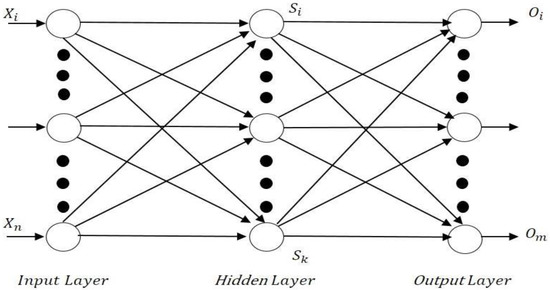
Figure 1.
An MLP with one hidden node.
- Weighted sum of inputs is given by:
- Outputs of hidden layers are calculated as:
- Final output based on the hidden node outputs is given as:
From the above equations, it can be seen that weights and thresholds define the final value of the MLPs. The major concern is finding optimum weights and thresholds (biases) for achieving a balanced relation between input and outputs.
3. Basic Cuckoo Search and Flower Pollination Algorithm
3.1. Cuckoo Search Algorithm
The CS algorithm is inspired by the obligatory brood parasitism behavior of cuckoos [35]. The cuckoos of some species lay their eggs in the nests of host birds, following an obligate brood parasitism. CS is a competitive algorithm among existing algorithms. CS contains components including the selection of best solution and ensuring that this best solution is passed on to the next generation. It employs local random walk to perform the exploitation locally and randomization via Lévy flights to perform the exploration globally. Three rules are established that describe the Cuckoo Search in a simple way. These are explained as follows:
- Each cuckoo lays one egg and dumps it in a random nest;
- The nest with highest fitness will carry over to next generation;
- The host bird discovered the cuckoo’s egg with a probability pa ∈ [0, 1]. A fixed number of host nests are available. Depending on , a new nest is built by the host bird at a new location either by throwing the egg away from the nest or abandoning the nest.
In CS, a solution is an egg that is already present in a nest and a new solution is that egg which is laid by a cuckoo. The not-so-good solutions of nests are replaced by the new and better solutions [35]. More complicated cases arise when multiple eggs are present in each nest. In these cases, the extended form of this algorithm can be used. Based on the above three rules, Equation (5) derives the Levy flight that is performed to produce a new solution for cuckoo:
where the previous solution is denoted by , is entry wise multiplication, and α > 0 is the step size. In most cases, α = 1 is used. The above equation is the stochastic equation for random walk. In the case of random walk, the current location draws a path to next status/location and the transition probability of next position. PSO also used this type of entry-wise product.
Cuckoos usually search for food using a basic random walk. This is a Markov chain whose updated position is determined by the present location and the transition probability of the following position. The performance of CS is enhanced using Lévy flights [36]. Lévy flight is a random walk measured in step-lengths following a heavy-tailed probability distribution. Ultimately, Levy flight is not a continuous space; it is used to refer to a discrete grid [37,38,39]. The Levy flight is employed in this study as a result of Levy flight’s greater efficiency in exploring the search space. Our algorithm is generated from a Levy distribution with infinite mean and variance.
As the random walk occurs via Lévy flight, the Lévy distribution draws the random step length as:
This random walk process is a heavy tail step-length distribution. The Lévy walk achieves new solutions nearer to the best solutions to speed up the local search [36]. Far field randomization should be used to create some of the solutions in order to prevent the system getting stuck in a local optimum. Here, some points are discussed that show that CS is analogous to and competitive with other optimization algorithms. First, as with other GA and PSO algorithms, CS is a population-based algorithm. Second, because of the heavy tailed step length, the large step is possible in CS and the randomization is more efficient. Third, a wide class of optimization problems have adapted to the CS because it tunes fewer parameters when compared to PSO and GA.
3.2. Flower Pollination Algorithm
Flowers are fascinating species. Dating from the Cretaceous period, flowers are estimated to comprise about 80 percent of the total species of plants [40]. About 250,000 species of flowers have been found on earth. The ultimate aim of flowers is to reproduce and this reproduction occurs mainly by pollination. In pollination, pollen is transferred from one flower to other by pollinators. Cross-pollination means that pollination occurs due to pollen from different plants. On the other hand, self-pollination means fertilization of pollen from the same or different flowers of the same plant. Pollinators can be insects, birds, or any other animal. Some flowers do attract only specific kinds of insects for pollination, showing a sort of flower-insect partnership; this is referred to as called flower constancy. Pollinators such as honeybees have been found to develop flower constancy. This property helps pollinators to visit only particular plant species, hence increasing the chances of reproduction for the flower and, in turn, maximizing nectar supply for the pollinator [41].When the pollen is shifted by pollinators such as insects and animals, the process is called biotic pollination (about 90 percent occurs via biotic). Meanwhile, when it occurs via diffusion or wind, the process is called abiotic [42] (this constitutes about 10 percent of pollination). In total, there are about 200,000 varieties of pollinators found on earth. Biotic cross-pollination occurs over long distance and is facilitated by birds, bats, bees, and fireflies, among other animals. This is often referred to as global pollination. Meanwhile, self-pollination is termed as local pollination.
The above characteristics are idealized into four set of rules [43]:
- Global pollination arises via biotic and cross-pollination.
- Local pollination occurs via abiotic and self-pollination.
- Flower constancy, termed as reproduction probability, is proportional to the similarity of two flowers.
- Switch probability p ϵ [0, 1] balances global and local pollination.
When designing the algorithm, it is expected that each plant has only one flower producing only a single pollen gamete. Following this, we can use yi as a solution equivalent to a flower or a pollen gamete, defining a single objective problem.
The above characteristics have been combined to design an FPA that mainly consists of local and global pollination. In the earlier version, pollination and reproduction of the fittest flower is ensured and the rules are represented mathematically as:
where is the current best solution, is the potential solution at t iteration, and α is the scaling factor to control the Lévy flight-based step size L(λ). Lévy flight is expressed as:
where Γ(λ) is the standard gamma function.
The local pollination rule can be mathematically represented as:
where and are pollens from diverse flowers of the same plants. In the confined space, flower constancy corresponds to a local random walk, and is selected from a uniform distribution in [0, 1].
4. Cuckoo Flower Search Algorithm
4.1. Algorithm Definition
The CFS algorithm is proposed as a hybrid version of the CS and FPA algorithms. Both these algorithms work in coordination to attain a global optimum solution. The main idea is to generate the current best solution for both cuckoos and flower pollinators. After finding this solution, both are compared, the best solution is considered, and the process is repeated. The solution after first evaluation is fed back to the cuckoos and flower pollinators. This procedure is continued until the termination criteria are met. The final solution is the most appropriate solution to the problem under discussion. There are three phases to the proposed CFS algorithm:
Initialization
This is the first phase of the CFS algorithm, in which the population is randomly initialized. The solution is initialized according to Equation (10) and operates as a potential solution to the problem under examination, starting with an initial population of N cuckoos and flower pollinators (termed as CF).
where i ϵ {1,….CF}, j ϵ {1,…..D}, CFi,j is the ith solution in the jth dimension, D is the dimension or number of variables in the problem being studied, CFmin,j, CFmax,j are the lower and upper bounds, respectively, and is randomly generated number between [0, 1]. Here, the population initialized in Equation (10) is same for both cuckoos and flower pollinators. The fitness of the solution is estimated for objective function after initialization, and the best solution attained is treated as the initial best for all cuckoos () and flower pollinators .
- Solution generation
After the initial step, two new solutions are generated: one solution is inspired by cuckoo brood parasitism and the other from flower pollinators. The main concern here is to follow exploration and exploitation in a well-defined fashion. In cuckoos, exploration is achieved by randomization via Lévy flights. Local random walk is used to achieve exploitation. The new solution is generated as per Equation (6) and its fitness is evaluated for the optimization problem being tested. The solution obtained in this manner is compared with the , and the best () among them is retained.
In the case of flower pollinators, exploration and exploitation is balanced by local pollination and global pollination, respectively. Equations (7) and (9), based on random probability in the search domain [0, 1], often called the switch probability, are used extensively to find the second new solution ). This solution and the initial best solution are also compared, resulting in another best solution among them.
- Final evaluation
After comparing the best fit solutions obtained by cuckoos () and flower pollinators (), the best solution attained is the final optimum solution. For both cuckoos and flower pollinators, the solution generated at the last stage is set as the initial best ( and , respectively) Unless and until the termination requirements are met, the same procedure is followed. The final solution obtained in this manner is the most appropriate solution. It is also worth noting that cuckoos and flower pollinators are both seeking the most appropriate solutions in parallel. If a cuckoo-produced solution becomes trapped in the local optimum and is unable to deliver the global optimal, flower pollinators assist it in exiting the local trap and achieving the global optimum, and vice versa. This characteristic increases the likelihood of the CFS algorithm reaching the global optimum solution.
Both CS and FPA are good algorithms in terms of finding global optimum solution, but the real problem is their inconsistency in finding the best fit individual every time the algorithm is run. This inconsistency is due to the problem of getting stuck in local optima while moving toward global optima. As a result, a better solution is required to move the algorithm closer to the global optimum. If the CS algorithm becomes stuck, FPA moves it towards the global optimum, and vice versa. As a result, both Cuckoos and Flower Pollinators collaborate analytically to obtain a global optimum. Figure 2 shows the flow code for the CFS algorithm. The pseudocode of the proposed algorithm is given in Algorithm 1.
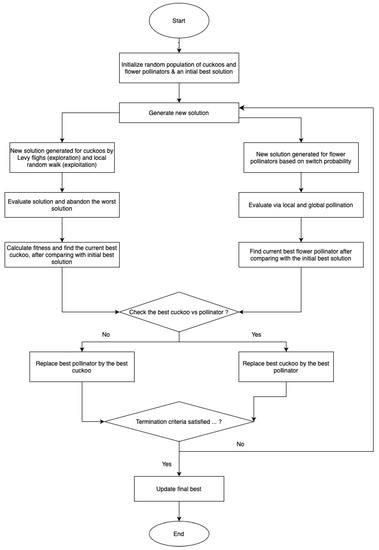
Figure 2.
Flow-code for CFS algorithm.
| Algorithm 1: Pseudocode of CFS algorithm |
| begin: 1. Initialize: , maximum iterations 2. Define Population, objective function f(x) 3. While (t < maximum iterations) For i = 1 to n For j = 1 to n Evaluate new solution using CS inspired equation; Evaluate new solution using FPA inspired equation; Find the best among the two using greedy selection; End for j End for i 4. Update current best. 5. End while 6. Find final best end. |
4.2. CFS-MLP Trainer
When training a MLP, the first step is to formulate a problem [44] and find values of weights and biases with the highest accuracy/classification/statistical results. These should be found by a trainer. This important step is achieved by training an MLP using meta-heuristic algorithms. There are three methods for training MLPs using meta-heuristic algorithms [45]:
- To find combination of weights and biases of MLP for achieving the minimum error using meta-heuristic algorithms. In this approach, proper values of weights are found without changing the basic architecture of the heuristic algorithm. It has simple a encoding phase and a difficult decoding phase, and so is often used for simple NNs.
- To find proper architecture for an MLP using heuristic algorithms. In this method, the architecture varies and it can be achieved by varying the connections between hidden nodes, layers, and neurons, as proposed in [46]. This method has a simple decoding phase but, due to complexity in the encoding phase, it is used for complex structures.
- To tune the gradient-based learning algorithm parameters using a heuristic approach. This method has been used to train FNNs using EAs [47] and others, such as GA [48], using a combination of methods to tune FNN. In this method, the decoding and encoding processes are very complicated and hence the structure becomes very complex.
In the present work, the CFS algorithm is proposed and applied to train an MLP using the first method. The weights and biases for the CFS algorithm are given in the form of a vector as follows:
where n is the number of nodes, Wij is the weight connection between ith and jth node, and is the bias of jth hidden node. After setting the initial variables, the fitness function is to be designed using CFS algorithm. This is achieved by defining a common metric for evaluation of the MLP and is called Mean Square Error (MSE). The MSE is used to calculate the difference between the desired output and the value obtained from MLP. The performance of MLP is based upon the average MSE values of all training samples and is given by:
where s is training samples count, m is the number of outputs, and and are the actual output and desired output of the ith input for the kth training sample, respectively. Based on MSE, the final objective function can be formulated as:
The overall process of using the CFS algorithm delivers MLP with weights as well as biases and, in turn, receives average MSE for all training samples. The CFS algorithm updates the weights and biases iteratively in order to achieve minimized average MSE. The best MSE is obtained from the last iteration of the algorithm. Since weights and biases find the best MSE in the MLP, there is a greater chance of improvement in the MLP structure at each iteration. Thus, the CFS algorithm converges toward a better solution than initial random solution.
5. Result and Discussion
This section presents the details on the applicability of the proposed CFS algorithm for classical benchmark problems and real-world optimization of FNN-MLP. We have used 19 benchmark functions, consisting of unimodal, multi-modal, and fixed dimension problems. For the optimization of real-world FNN-MLP, five highly challenging datasets have been used. More details on applicability are presented in the consecutive subsections. For performance analysis, the simulations are performed on MATLAB, using a Windows 10 × 64, Intel Core i3 processor, with 8 GB RAM.
5.1. Benchmark Problems
To check the effectiveness of the CFS algorithm, it was tested on nineteen well known benchmark problems. The Wilcoxon rank-sum tests were performed to test the validity of results statistically. This non-parametric test is used to detect the static significance of any algorithm. Differences between two pairs of populations were analyzed and compared. The test returns a p-value determining the significance level of two algorithms. This value should be less than 0.05 for an algorithm to be statistically efficient [49]. The proposed algorithm is compared with ABC [50], Firefly Algorithm [51], FPA, CS, and Bat Flower Pollinator [52] algorithms. The parameter setting to test each algorithm for benchmark problems is shown in Table 1.

Table 1.
Parameter settings for various algorithms.
5.1.1. Unimodal Functions
There is no local solution for unimodal functions; they have a single global solution. These benchmark functions are useful for evaluating the convergence characteristics of heuristic optimization techniques. The CFS algorithm was applied to four unimodal benchmark problems with three dimension sets (30, 50, and 100), as given in Table 2. The CFS algorithm was compared to the ABC, FA, FPA, CS, and BFP algorithms (see Table 3, Table 4, Table 5, Table 6, Table 7 and Table 8). For the 30 (Table 3) and 50 (Table 5) dimension (D) problems, with the function f1, the FPA algorithm has a better mean and best value but CS and CFS are found to give the best values of standard deviation. For function f2, the FA is found to be better, with a highly competitive result for the CFS algorithm. for f3, the CFS algorithm provides better results, and for f4, the ABC and CFS algorithms are both competitive when compared to rest of the algorithms. For 100 D (Table 7), the CFS algorithm performs better for f2 and f3. for f1, FPA is better, and for f4, ABC is better. The BFP algorithm is better for none of the functions. The rank-sum tests from Table 4, Table 6 and Table 8 acknowledge the superior performance of the CFS algorithm. The convergence characteristics are shown in Figure 3.
Table 2.
Description of Unimodal Test functions.
Table 3.
Results comparison for unimodal functions (30 Dimension).
Table 4.
P-test values of simulated algorithms for unimodal functions (30 Dimension).
Table 5.
Results comparison for unimodal functions (50 Dimension).
Table 6.
P-test values of simulated algorithms for unimodal functions (50 Dimension).
Table 7.
Results comparison for unimodal functions (100 Dimension).
Table 8.
P-test values of simulated algorithms for unimodal functions (100 Dimension).
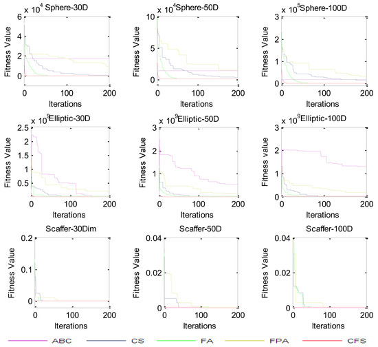
Figure 3.
Convergence curves for unimodal functions.
5.1.2. Multimodal Functions
Multimodal benchmark functions feature several local minima that grow in number exponentially with dimension. As such, they are good for testing an algorithm’s ability to avoid local minima. The CFS algorithm has been applied to six multimodal benchmark problems, with three-dimension sets (30, 50, and 100), as shown in Table 9. The algorithm has been compared to the ABC, FA, FPA, BFP, and CS algorithms. For 30 D and 50 D problems, with the f5, f6, and f7 functions, the CFS algorithm performs better, while only the FA algorithm performs better than CFS with the f8, f9, and f10 functions, as shown in Table 10, Table 11, Table 12 and Table 13, respectively. For 100 D (Table 14 and Table 15), the CFS algorithm performs better for the f5, f6, f7, and f9 functions. for f8 and f10, the FA algorithm performs better. The rank-sum tests from Table 11, Table 13 and Table 15 shows that the performance of the CFS algorithm is better statistically. The convergence characteristics are shown in Figure 4.
Table 9.
Description of multimodal test problems.
Table 10.
Results comparison for multimodal functions (30 Dimension).
Table 11.
P-test values of various algorithms for multimodal functions (30 Dimension).
Table 12.
Results comparison for multimodal functions (50 Dimension).
Table 13.
P-test values of various algorithms for multimodal functions (50 Dimension).
Table 14.
Results comparison for multimodal functions (100 Dimension).
Table 15.
P-test values of various algorithms for multimodal functions (100 Dimension).
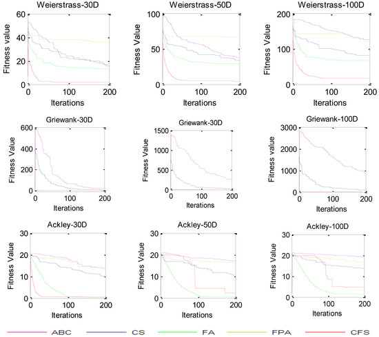
Figure 4.
Convergence curves for multimodal functions.
5.1.3. Fixed Dimension Functions
Fixed dimension benchmark functions have finite dimensional space. The CFS algorithm has been applied to nine benchmark functions, as shown in Table 16, and the results have been compared to the ABC, CS, FA, BFP, and FPA algorithms. It can be seen from Table 17 and Table 18 that the CFS algorithm performs better than the other algorithms for all the test problems. For functions f14, f15, f16, f17, and f18, the ABC, FA, FPA, and CS algorithms are not able to achieve the global optimum. For the remaining algorithms, even if the global optimum is met, the CFS algorithm shows superior consistency because of its better standard deviation. The CFS algorithm’s results are also statistically better, as shown in Table 18. The convergence curves are shown in Figure 5.
Table 16.
Description of fixed dimension test functions.
Table 17.
Results comparison for fixed dimension functions.
Table 18.
P-test values of various algorithms for fixed dimension functions.
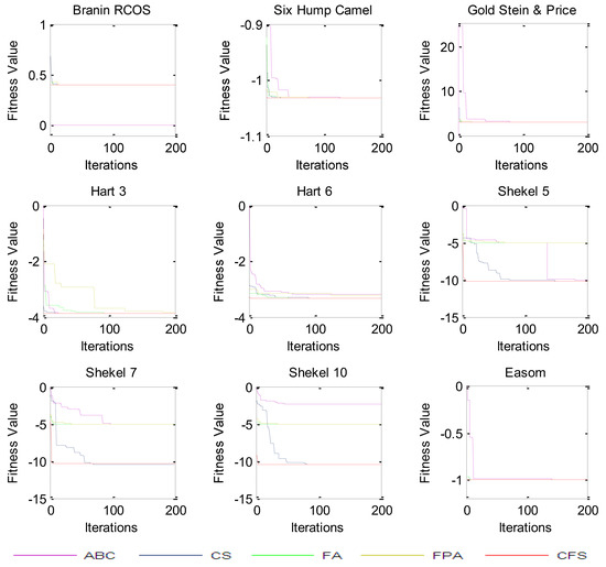
Figure 5.
Convergence curves for fixed dimension problems.
5.2. FNN–MLP Datasets
The proposed CFS algorithm was used to train FNN-MLP datasets. The standard benchmark FNN–MLP data sets were obtained from the Machine Learning Repository of the University of California, Irvine [53]. The datasets used are: Breast Cancer, XOR, Balloon, Iris, and Heart. The results are compared with the PSO, GA, ES, ACO, GWO, PLIB [30,54,55,56,57] algorithms, and the Whale Optimization Algorithm (WOA) [58] and the Moth Flame Optimization (MFO) [59] for verification. The optimization parameter settings for the CFS algorithm are presented in Table 19. Table 20 details the specifications of the datasets used for comparison. The simplest dataset is the 3-bit XOR; it has three attributes and eight training/test samples. for the Balloon dataset, there are four attributes and 16 training/test samples. For the Iris dataset, there are 150 training/test samples with four attributes. For the Breast Cancer dataset, the highest number of 100 test samples, 599 training samples, and nine attributes are used. for the Heart dataset, there are 80 training samples, 187 test samples, and 22 attributes. The number of classes for each dataset is two, except for Iris, which is set to three. These datasets are highly complex sets of problems and are employed to test the performance of the CFS algorithm. The total number of runs for the CFS algorithm is set to 10; this is the same as used in study [30]. The number of function evaluations for the XOR and Balloon datasets is 50 × 250 = 12,500 for all the algorithms. For the Iris, Breast Cancer, and Heart datasets, the number of function evaluations is 20 × 250 = 5000 for the CFS algorithm and 200 × 250 = 50,000 for the rest. The results are presented in the form of an average of 10 runs and their standard deviation is obtained from the best MSEs in the last iteration of the CFS algorithm. The best results are those with the lowest average and standard deviation, ultimately indicating the better performance of the proposed approach [60,61].
Table 19.
Parameters for algorithms.
Table 20.
Classification datasets.
The number of hidden nodes for N number of inputs of datasets is kept constant and is given by . The structure for each MLP is given in Table 21.
Table 21.
MLP structure for each dataset.
5.2.1. XOR Dataset
This dataset returns XOR of input as output. It has three inputs, eight training/test samples, and one output. This dataset has a dimension of 36 with range of [−10, 10], with an MLP structure of 3−7−1. The results, in term of average and standard deviation, are given in Table 22. It can be seen in Table 4 that the performance evaluation of the CFS-MLP algorithm is far better than all other algorithms tested.
Table 22.
Comparison results of CFS-MLP for XOR dataset.
5.2.2. Balloon Dataset
The Balloon dataset has a dimension of 55, with range of [−10, 10]. This dataset has 18 training/test samples, with four attributes and two classes, with an MLP structure of 4−9−1. The results are given in Table 23. The results show that the CFS algorithm gives far higher average and standard deviation values when compared to the GWO, PSO, GA, ACO, ES, PBIL, WOA, and MFO algorithms.
Table 23.
Comparison results of CFS-MLP for the Balloon dataset.
5.2.3. Iris Dataset
The Iris dataset has 75 variables to be optimized in the range of [−10, 10]. It has 150 training/test samples, with four attributes and two classes. The MLP structure of 4−9−3 is utilized to solve this dataset. The results are shown in Table 24. For the Iris dataset, the results of the CFS algorithm are competitive with GWO in terms of average; for standard deviation, the results of the CFS algorithm are superior.
Table 24.
Comparison results of CFS-MLP for the Iris dataset.
5.2.4. Breast Cancer Dataset
This is a challenging dataset, with 100 test samples, 599 training samples, nine attributes, and two classes. It has 209 dimensions, with an MLP structure of 9−19−1. The outcomes of this dataset are given in Table 25. The results show that the CFS algorithm is far superior than the PSO, GA, ACO, PBIL, WOA, and MFO algorithms. When compared to GWO, they are highly competitive.
Table 25.
Comparison results of CFS-MLP for the Breast Cancer dataset.
5.2.5. Heart Dataset
This is the last dataset used in this paper and was solved with an MLP structure of 22−45−1. It has 187 test samples, 80 training samples, 22 attributes, and two classes. The results are shown in Table 26. The Heart dataset is a very challenging dataset, with a 1081 dimension. The CFS algorithm performs better for this dataset when compared to others.
Table 26.
Comparison results of CFS-MLP for the Heart dataset.
5.3. Discussion of Results
The results comparison of the CFS algorithm with the ABC, CS, FA, FPA, and BFP algorithms show that, for test function, the CFS algorithm delivers very competitive results for unimodal and multimodal benchmark problems. For fixed dimension problems, no algorithm among ABC, CS, FA, FPA, and BFP are comparable. This occurs as a result of the inability of these algorithms to emerge from local minima. The ABC algorithm has the problem of becoming stuck in local minima, while the CS and FPA algorithms are inconsistent due to their inability to emerge from local minima and are, hence, inconsistent. In its initial stage, the FA algorithm has slower convergence because of random distribution and as a result of its insufficiency in exploring ability. At the last stage, fireflies gather around the optimal solution but, due to random motion and attractiveness, there can be flight mistake and hence the solution converges very slowly.
The results of the CFS-MLP clearly show that, for the XOR and Balloon datasets, there are same number of function evaluations and that the results are bothbetter and significant. For the Iris, Breast Cancer, and Heart datasets, the minimum number of function evaluations for CFS algorithms is 5000, while for others it is 50,000. Hence, it can be said that the CFS algorithm is able to achieve a more significant result with fewer function evaluations. This proves the superiority of the CFS algorithm over the GWO, PSO, GA, ACO, ES, PBIL, WOA, and MFO algorithms.
In the CFS algorithm, there are two search agents: cuckoos and flower pollinators. When cuckoos are not able to find the optimal solution, flower pollinators help them; in turn, the flower pollinators are helped by cuckoos when stuck in a local optimum. Therefore, two solutions (one from cuckoos and the other from flower pollinators) are generated. The final solution is the best among the two. This helps the CFS algorithm to achieve faster convergence and consistency in finding the optimal solution.
6. Conclusions
In this work, a new CFS algorithm was proposed for MLP training. The algorithm was first tested over 19 standard benchmark functions and their results were statistically compared with the ABC, CS, FA, FPA, and BFP algorithms. The results demonstrate that the CFS algorithm perform significantly better, with higher consistency, in avoiding local minima when compared to the ABC, CS, FA, FPA, and BFP algorithms. The CFS algorithm was then used to train MLPs; five datasets were used. The results of the CFS-MLP were compared, in terms of average and standard deviation, with the GWO, PSO, GA, ACO, ES, PBIL, WOA, and MFO algorithms. The experimental results again proved the superiority of the CFS algorithm for MLPs.
Despite this, the proposed algorithm has certain drawbacks. Because of the stochastic nature of the algorithm, the algorithm is inefficient for several kinds of problems. As the CFS algorithm uses two general equations for finding new solutions, the computational complexity of the algorithm increases. Thus, it is imperative to find new and prospective solutions to deal with the complexity problem. As a future direction of study, the parameters of the algorithm can be exploited to find the best set of parameters. In addition, the CFS algorithm can be applied to various other domains, including clustering, antenna array synthesis, feature selection, medical imaging, segmentation, and others. Apart from that, the proposed algorithm can be extended to multi-objective, hyper-parameters, and other dimensions.
Author Contributions
Conceptualization, R.S.; methodology, R.S.; software, N.M.; validation, R.S., N.M. and V.M.; formal analysis, V.M.; investigation, R.S.; resources, N.M.; data curation, V.M.; writing—original draft preparation, R.S.; writing—review and editing, R.S, and N.M.; visualization, R.S.; supervision, R.S.; project administration, R.S. and N.M.; All authors have read and agreed to the published version of the manuscript.
Funding
This research received no external funding.
Data Availability Statement
Data will be made available on request.
Conflicts of Interest
The authors declare no conflict of interest.
References
- McCulloch, W.S.; Pitts, W. A logical calculus of the ideas immanent in nervous activity. Bull. Math. Biophys. 1943, 5, 115–133. [Google Scholar] [CrossRef]
- Kohonen, T. The self-organizing map. Proc. IEEE 1990, 78, 1464–1480. [Google Scholar] [CrossRef]
- Dorffner, G. Neural networks for time series processing. Neural Netw. World 1996. [Google Scholar]
- Ghosh-Dastidar, S.; Adeli, H. Spiking neural networks. Int. J. Neural Syst. 2009, 19, 295–308. [Google Scholar] [CrossRef] [PubMed]
- Bebis, G.; Georgiopoulos, M. Feed-forward neural networks. IEEE Potentials 1994, 13, 27–31. [Google Scholar] [CrossRef]
- Rosenblatt, F. The Perceptron, A Perceiving and Recognizing Automaton Project Para; Cornell Aeronautical Laboratory: Buffalo, NY, USA, 1957. [Google Scholar]
- Werbos, P. Beyond Regression: New Tools for Prediction and Analysis in the Behavioral Sciences. Ph.D. Thesis, Harvard University, Cambridge, MA, USA, 1974. [Google Scholar]
- Reed, R.D.; Marks, R.J. Neural Smithing: Supervised Learning in Feedforward Artificial Neural Networks; MIT Press: Cambridge, MA, USA, 1998. [Google Scholar]
- Caruana, R.; Niculescu-Mizil, A. An empirical comparison of supervised learning algorithms. In Proceedings of the 23rd International Conference on Machine Learning, Pittsburgh, PA, USA, 25–29 June 2006; pp. 161–168. [Google Scholar]
- Hinton, G.E.; Sejnowski, T.J. Unsupervised Learning: Foundations of Neural Computation; MIT Press: Cambridge, MA, USA, 1999. [Google Scholar]
- Wang, D. Unsupervised Learning: Foundations of Neural Computation; MIT Press: Cambridge, MA, USA, 2001; p. 101. [Google Scholar]
- Hertz, J. Introduction to the Theory of Neural Computation. Basic Books 1; Taylor Francis: Abingdon, UK, 1991. [Google Scholar]
- Wang, G.-G.; Guo, L.; Gandomi, A.H.; Hao, G.-S.; Wang, H. Chaotic krill herd algorithm. Inf. Sci. 2014, 274, 17–34. [Google Scholar] [CrossRef]
- Wang, G.-G.; Gandomi, A.H.; Alavi, A.H.; Hao, G.-S. Hybrid krill herd algorithm with differential evolution for global numerical optimization. Neural Comput. Appl. 2013, 25, 297–308. [Google Scholar] [CrossRef]
- Van Laarhoven, P.J.; Aarts, E.H. Simulated Annealing; Springer: Berlin/Heidelberg, Germany, 1987. [Google Scholar]
- Szu, H.; Hartley, R. Fast simulated annealing. Phys. Lett. A 1987, 122, 157–162. [Google Scholar] [CrossRef]
- Mitchell, M.; Holland, J.H.; Forrest, S. When will a genetic algorithm outperform hill climbing? NIPS 1993, 51–58. [Google Scholar]
- Sanju, P. Enhancing Intrusion Detection in IoT Systems: A Hybrid Metaheuristics-Deep Learning Approach with Ensemble of Recurrent Neural Networks. J. Eng. Res. 2023; in press. [Google Scholar]
- Mirjalili, S.; Mohd Hashim, S.Z.; Moradian Sardroudi, H. Training feedforward neural networks using hybrid particle swarm optimization and gravitational search algorithm. Appl. Math. Comput. 2012, 218, 11125–11137. [Google Scholar] [CrossRef]
- Whitley, D.; Starkweather, T.; Bogart, C. Genetic algorithms and neural networks: Optimizing connections and connectivity. Parallel Comput. 1990, 14, 347–361. [Google Scholar] [CrossRef]
- Shokouhifar, A.; Shokouhifar, M.; Sabbaghian, M.; Soltanian-Zadeh, H. Swarm intelligence empowered three-stage ensemble deep learning for arm volume measurement in patients with lymphedema. Biomed. Signal Process. Control. 2023, 85, 105027. [Google Scholar] [CrossRef]
- Socha, K.; Blum, C. An ant colony optimization algorithm for continuous optimization: Application to feed-forward neural network training. Neural Comput. Appl. 2007, 16, 235–247. [Google Scholar] [CrossRef]
- Ozturk, C.; Karaboga, D. Hybrid Artificial Bee Colony algorithm for neural network training. In Proceedings of the 2011 IEEE Congress on, Evolutionary Computation (CEC), New Orleans, LA, USA, 5–8 June 2011; pp. 84–88. [Google Scholar]
- Mendes, R.; Cortez, P.; Rocha, M.; Neves, J. Particle swarms for feed forward neural network training. In Proceedings of the 2002 International Joint Conference on Neural Networks. IJCNN’02 (Cat. No.02CH37290), Honolulu, HI, USA, 12–17 May 2002. [Google Scholar]
- Gudise, V.G.; Venayagamoorthy, G.K. Comparison of particle swarm optimization and backpropagation as training algorithms for neural networks. In Proceedings of the Swarm Intelligence Symposium, SIS’03, Indianapolis, IN, USA, 26 April 2003; pp. 110–117. [Google Scholar]
- Ilonen, J.; Kamarainen, J.-K.; Lampinen, J. Differential evolution training algorithm for feed-forward neural networks. Neural Process. Lett. 2003, 17, 93–105. [Google Scholar] [CrossRef]
- Uzlu, E.; Kankal, M.; Akpınar, A.; Dede, T. Estimates of energy consumption in Turkey using neural networks with the teaching–learning-based optimization algorithm. Energy 2014, 75, 295–303. [Google Scholar] [CrossRef]
- Moallem, P.; Razmjooy, N. A multi-layer perceptron neural network trained by invasive weed optimization for potato color image segmentation. Trends Appl. Sci. Res. 2012, 7, 445–455. [Google Scholar] [CrossRef]
- Darekar, R.V.; Chavan, M.; Sharanyaa, S.; Ranjan, N.M. A hybrid meta-heuristic ensemble based classification technique speech emotion recognition. Adv. Eng. Softw. 2023, 180, 103412. [Google Scholar] [CrossRef]
- Mirjalili, S. How effective is the Grey Wolf Optimizer in training multi-layer perceptrons. Appl. Intell. 2015, 43, 150–161. [Google Scholar] [CrossRef]
- Yang, X.-S.; Deb, S. Engineering optimization by cuckoo search. Int. J. Math. Model. Numer. Optim. 2010, 1, 330–343. [Google Scholar]
- Yang, X.-S. Flower Pollination Algorithm for Global Optimization. In Proceedings of the 11th International Conference, UCNC 2012, Orléan, France, 3–7 September 2012; Volume 7445, pp. 240–249. [Google Scholar] [CrossRef]
- Fine, T.L. Feedforward Neural Network Methodology; Springer: Berlin/Heidelberg, Germany, 1999. [Google Scholar]
- Mirjalili, S.; Sadiq, A.S. Magnetic optimization algorithm for training multi-layer perceptron. In Proceedings of the Communication Software and Networks (ICCSN), 2011 IEEE 3rd International Conference, Xi’an, China, 27–29 May 2011; pp. 42–46. [Google Scholar]
- Payne, R.B.; Sorenson, M.D.; Klitz, K. The Cuckoos; Oxford University Press: Oxford, UK, 2005. [Google Scholar]
- Barthelemy, P.; Bertolotti, J.; Wiersma, D.S. A Lévy flight for light. Nature 2008, 453, 495–498. [Google Scholar] [CrossRef]
- Yang, X.-S.; Deb, S. Cuckoo Search via Levy Flights’. In Proceedings of the 2009 World Congress on Nature & Biologically Inspired Computing (NaBIC), Coimbatore, India, 9–11 December 2009; IEEE Publications: Piscataway, NJ, USA, 2009. [Google Scholar]
- Brown, C.; Liebovitch, L.S.; Glendon, R. Lévy Flights in Dobe Ju/’hoansi Foraging Patterns. Human Ecol. 2007, 35, 129–138. [Google Scholar] [CrossRef]
- Pavlyukevich, I. Cooling down Lévy flights. J. Phys. A Math. Theory 2007, 40, 12299–12313. [Google Scholar] [CrossRef]
- Walker, M. How Flowers Conquered the World, BBC Earth News, 10 July 2009. Available online: http://news.bbc.co.uk/earth/hi/earth_news/newsid_8143000/8143095.stm (accessed on 1 January 2019).
- Waser, N.M. Flower constancy: Definition, cause and measurement. Am. Nat. 1986, 127, 596–603. [Google Scholar] [CrossRef]
- Glover, B.J. Understanding Flowers and Flowering: An Integrated Approach; Oxford University Press: Oxford, UK, 2007. [Google Scholar]
- Xin-She, Y.; Karamanoglu, M.; He, X. Flower pollination algorithm: A novel approach for multiobjective optimization. Eng. Optim. 2014, 46, 1222–1237. [Google Scholar]
- Belew, R.K.; McInerney, J.; Schraudolph, N.N. Evolving Networks: Using the Genetic Algorithm with Connectionist Learning; Cognitive Computer Science Research Group: La Jolla, CA, USA, 1990. [Google Scholar]
- Smizuta, T.; Sato, D.; Lao, M.; Ikeda, T. Shimizu, Structure design of neural networks using genetic algorithms. Complex Syst. 2001, 13, 161–176. [Google Scholar]
- Yu, J.; Wang, S.; Xi, L. Evolving artificial neural networks using an improved PSO and DPSO. Neurocomputing 2008, 71, 1054–1060. [Google Scholar] [CrossRef]
- Leung, F.H.; Lam, H.; Ling, S.; Tam, P.K.S. Tuning of the structure and parameters of a neural network using an improved genetic algorithm. IEEE Trans. Neural Netw. 2003, 14, 79–88. [Google Scholar] [CrossRef]
- Montana, D.J.; Davis, L. Training Feedforward Neural Networks Using Genetic Algorithms. IJCAI 1989, 89, 762–767. [Google Scholar]
- Derrac, J.; García, S.; Molina, D.; Herrera, F. A practical tutorial on the use of nonparametric statistical tests as a methodology for comparing evolutionary and swarm intelligence algorithms. Swarm Evolut. Comput. 2011, 1, 3–18. [Google Scholar] [CrossRef]
- Karaboga, D. An Idea Based on Honey Bee Swarm for Numerical Optimization; Technical Report TR-06; Erciyes University, Engineering Faculty, Computer Engineering Department: Kayseri, Turkey, 2005. [Google Scholar]
- Yang, X.S. Firefly algorithms for multimodal optimization. In Stochastic Algorithms: Foundations and Applications; Lecture Notes in Computer Sciences; SAGA: Chicago, IL, USA, 2009; Volume 5792, pp. 169–178. [Google Scholar]
- Urvinder, S.; Salgotra, R. Synthesis of linear antenna array using flower pollination algorithm. Neural Comput. Appl. 2016, 29, 435–445. [Google Scholar]
- Blake, C.; Merz, C.J. {UCI} Repository of Machine Learning Databases; UCI: Aigle, Switzerland, 1998. [Google Scholar]
- Beyer, H.-G.; Schwefel, H.-P. Evolution strategies—A comprehensive introduction. Nat. Comput. 2002, 1, 3–52. [Google Scholar] [CrossRef]
- Yao, X.; Liu, Y.; Lin, G. Evolutionary programming made faster. Evol. Comput. IEEE Trans. 1999, 3, 82–102. [Google Scholar]
- Yao, X.; Liu, Y. Fast evolution strategies. In Proceedings of the Evolutionary Programming VI, Indianapolis, IN, USA, 13–16 April 1997; pp. 149–161. [Google Scholar]
- Baluja, S. Population-Based Incremental Learning: A Method for Integrating Genetic Search-Based Function Optimization and Competitive Learning; DTIC Document; Carnegie Mellon University: Pittsburgh, PA, USA, 1994. [Google Scholar]
- Seyedali, M.; Lewis, A. The whale optimization algorithm. Adv. Eng. Softw. 2016, 95, 51–67. [Google Scholar]
- Seyedali, M. Moth-flame optimization algorithm: A novel nature-inspired heuristic paradigm. Knowl. Based Syst. 2015, 89, 228–249. [Google Scholar]
- Zhou, Y.; Niu, Y.; Luo, Q.; Jiang, M. Teaching learning-based whale optimization algorithm for multi-layer perceptron neural network training. Math. Biosci. Eng. 2020, 17, 5987–6025. [Google Scholar] [CrossRef]
- Chong, H.Y.; Yap, H.J.; Tan, S.C.; Yap, K.S.; Wong, S.Y. Advances of metaheuristic algorithms in training neural networks for industrial applications. Soft Comput. 2021, 25, 11209–11233. [Google Scholar] [CrossRef]
Disclaimer/Publisher’s Note: The statements, opinions and data contained in all publications are solely those of the individual author(s) and contributor(s) and not of MDPI and/or the editor(s). MDPI and/or the editor(s) disclaim responsibility for any injury to people or property resulting from any ideas, methods, instructions or products referred to in the content. |
© 2023 by the authors. Licensee MDPI, Basel, Switzerland. This article is an open access article distributed under the terms and conditions of the Creative Commons Attribution (CC BY) license (https://creativecommons.org/licenses/by/4.0/).