An Analysis of the Determinants of Household Consumption Expenditure and Poverty in India


1
Department of Economics, Sogang University, Room GN702, 35 Baekbeom-ro, Mapo-gu, Seoul 04107, Korea
2
Department of Economics, College of Arts and sciences, Emory University, 201 Dowman Drive, Atlanta, GA 30322, USA
3
Asian Development Bank Institute, 6 ADB Avenue, Mandaluyong City 1550, Philippines
*
Author to whom correspondence should be addressed.
Economies 2019, 7(4), 96; https://doi.org/10.3390/economies7040096
Submission received: 27 June 2019
/
Revised: 29 August 2019
/
Accepted: 18 September 2019
/
Published: 20 September 2019
(This article belongs to the Special Issue Growth, Global Poverty Reduction and Income Distribution)
Abstract
:This article examines the determinants of household income among urban and rural areas in India and evaluates households’ performance with different characteristics in terms of poverty. It uses four rounds of data from the consumer expenditure survey (50th, 1993/1994; 55th, 1999/2000; 61st, 2004/2005; and 66th, 2009/2010) by the National Sample Survey Organization (NSSO) in the empirical section. This study consists of two main parts. In the first, it looks at the impact of the characteristics of the head of the household (age, educational level, marital status, and gender) and household characteristics (main occupational type, household size, and social status) on monthly per capita expenditure through conditional mean least squares (LS) regressions and conditional quantile regressions. Households headed by those who are older, married, belonging to lower castes, and living in less-developed states are more likely to be in poverty. In the second part, the article explores stochastic dominance rankings relative to large classes of welfare functions/preferences between pairwise sub-groups identified by the survey year, gender, social status, and occupational type of the household heads. Our results show that ‘inferior groups’ such as ‘Backward classes’, agricultural labor in rural areas, and casual labor in urban areas are vulnerable and may be targeted for poverty alleviation strategies. The first part sheds light on key determinants of household expenditure, while the second provides a picture of poverty outcomes which helps identify potential target groups for poverty-alleviation strategies.
JEL Classification:
C31; D63; O15; O181. Introduction
Poverty alleviation has been the goal of India’s income policy since its independence in 1947. Investments in human capital to raise labor productivity is one example of the goals of this policy. Despite three decades of good distributional intentions and constant piecemeal changes in policy, about half of the population in India has been struggling under the poverty line. Many have attributed the failure of poverty alleviation to the slow growth of the economy (a little above 1 percent) and constant increase in its population (more than 2 percent) prior to the 1980s (Panagariya 2008).
However, as the 1980s unfolded India started emerging out of the slow growth it had been experiencing till then. A survey by the government of India (2012) showed that between 1980 and 2010, India achieved an annual growth rate of 6.2 percent, while the world as a whole registered a growth rate of 3.3 percent. As a result, India’s share in global GDP more than doubled from 2.5 percent in 1980 to 5.5 percent in 2010, making it the fourth largest economy globally. India’s rank in per capita GDP showed an improvement from 117 in 1990 to 101 in 2000 and further to 94 in 2009. Fortuitously, this shift in the growth rate also coincided with a break in poverty trends. According to statistics from the National Sample Survey, the poverty ratio at the national level fell from 51.3 percent in 1977–1978 (Planning Commission 2002) to 29.8 percent in 2009–2010 (Planning Commission 2012).
However, some have raised doubts about this sharp decline in the poverty ratio. As a reforms skeptic, Sen (2000) was quick to point out that a critical change in the sample design introduced in the 55th Round (1993/1994) made the calculations non-comparable to those based on the earlier rounds. A more recent debate has focused on the change in the definition of poverty levels. Based on the price indices calculated from the 2009–2010 Household Consumer Expenditure Survey, the Suresh Tendulkar committee1 reduced the 2004–2005 poverty level from Rs 32 per day to Rs 28 per day. As a result, the poverty line was set at Rs 859.60 per month in urban regions and Rs 672.80 per month in rural regions.
Making judgments about the incidence of monetary poverty across time and space, or ranking the severity of poverty between sub-groups, necessitates making a substantial number of important methodological choices. Any empirical investigation of the poverty immediately faces the problems of setting the appropriate poverty line and choosing the proper poverty index since it is possible to portray conflicting pictures of ranking orders between sub-groups.
Duclos and Araar (2006) assert that most empirical studies focus on measuring and comparing cardinal indices of poverty.2 The main advantage of these indices is that they focus on only one or a few numerical assessments for ‘complete ordering’. Using this method, poverty and equity can be compared across different distributions. However, ordinal comparisons (Sen 1976)3 enable a comparison of indices across time, states, and socio-demographic characteristics, or comparisons of policy regimes and introduction of fiscal policy and macroeconomic adjustment programs. These two approaches may be sensitive to the subjective choice of indices and poverty lines, undermining one’s confidence in comparing distributions or in making policy recommendations.
It is worth mentioning that, as an advantage, the use of ordinal comparisons may avoid the difficulties in the choice of appropriate theoretical and econometric models and methods. Ordinal poverty comparisons provide ‘weak orders’ which can be robust in the choice of some measurement assumptions since they will be valid for wide classes and ranges of such assumptions. When the problem is simply to resolve which of the two approaches will better alleviate poverty, ordinal comparisons which may enable comparisons across different dimensions and characteristics of the population and policy regimes can be more informative in decision-making.
Ordinal comparisons of poverty involve using classes of distributive indices to find out whether an ordering of poverty is valid for all the indices that are members of a class of a specific order can be empirically tested through stochastic dominance tests. When two income distributions do not intersect, they can be ranked by first-order dominance. If they intersect, different indices may disagree about their ordering before and after policy (event) distributions. To resolve this ambiguity, we may move to ordering by second-order dominance, reflecting a class of preferences that prefers equality. In this case, the distributive indices obey additional ethical principles (other than anonymity and population invariance) of distribution sensitivity. As the order increases, the relative ethical weight assigned to the effect of income changes at the bottom of the distribution also increases. The corresponding indices become more sensitive to the distribution of income among the poorest and to movement out of poverty.
This study is an attempt to identify the important characteristics of vulnerable groups and to determine which observable socioeconomic characteristics are associated with reduction in poverty at the fastest rate. We first use parametric methods—conditional mean and conditional quantile regressions—to specify the models for the determinants of household consumption expenditure. We then apply non-parametric stochastic dominance tests to assess the performance of sub-groups in terms of poverty reduction with the aim of revealing any distributional rankings amongst the target groups over time. The two methods are different but complementary in analyzing consumption expenditure, which is close to the needs of the population and is smoother than income.
The first part of this paper looks at the impact of the household head and household characteristics on expenditure through conditional mean least squares and conditional quantile regressions. The results show that households headed by those who are older, married, belonging to lower castes, and living in less-developed states are more likely to be in poverty. The second part explores the use of stochastic dominance rankings between pairwise sub-groups identified by the survey year and various household head and household characteristics. The results show that the ‘Backward classes’, agricultural labor in rural areas, and casual labor in urban areas are among the most vulnerable and should be targeted for poverty alleviation strategies.
The two parts are complementary as the first sheds light on key determinants of household expenditure while the second provides a picture of poverty which helps identify the target groups to which the government can direct poverty alleviation strategies. Identification of key determinants of level and variations in households’ expenditure has relevance for poverty-reduction strategies. The non-parametric method provides information about distribution of consumption expenditure by different household characteristics but it does not shed light on the factors impacting the level and variations in the consumption and the quantification of their impact. Thus, a better understanding of household consumption expenditure is directly related to poverty by the determinants’ importance in selecting alternative ways to fine-tune policy to effectively reduce poverty among different sub-groups in targeted policies. The quantile regressions help distinguish between poor and non-poor behavior and responses to changes in individual determinants of consumption expenditure. Together with stochastic dominance, this empowers identification of the poor and their separation from the non-poor segments of the population. Therefore, identifying and estimating the effects of determinants of household expenditure and their effective use in policy design and implementation suggest the presence of direct relationships between the three methodologies and their complementarities.
This rest of this paper is organized as follows. Section 2 reviews and summarizes relevant literature on income poverty and the stochastic dominance analysis of income and poverty distribution. Section 3 introduces the data and the variables used in this research. Section 4 is an econometric study including the introduction of parametric models and a theoretical framework of poverty dominance. Section 5 presents the results of an analysis of income poverty in India. Section 6 gives a summary of the results and the conclusion.
2. Literature Review
There is voluminous literature available on poverty. This mainly focuses on unidimensional income- and consumption-based poverty. In recent years, greater attention has been paid to multidimensional poverty. In both these cases, a distinction is made between rural versus urban and developed versus developing countries. A choice is also made between absolute and relative poverty lines, and between fixed and variable relative poverty lines. The measured poverty rate is then explained by its possible determinants. Due to space limitations, our study focuses on a regression analysis of poverty variations and a distribution analysis of poverty using stochastic dominance. As alternative approach and in context of developing countries Fernández-Ramos et al. (2016) and Garza-Rodriguez et al. (2010) investigate the dynamics of poverty transition and chronic and transient poverty in Mexico.
Literature on stochastic dominance analyzing the distribution of income has developed rapidly. This development has been along a methodology that provides better tests for dominance in the income distribution and poverty analyses. There is an association between unequal distribution of income and relative poverty. In their analysis of poverty and equity, Duclos and Araar (2000) provide a comprehensive review of the measurement, policy, and estimation issues. Anderson (1993) discusses the non-parametric tests of stochastic dominance in income distribution. In recent years, studies have also provided empirical evidence on the use of the methodology and its usefulness. Deaton and Dreze (2002) re-examine poverty and inequality in India. Araar (2006) discusses theory and practices of poverty, inequality, and stochastic dominance with illustrations based on surveys in Burkina Faso. Chin and Prakash (2011) look at the redistributive effects of political reservations on minorities in India. Fan et al. (2000) study the effects of government spending, growth, and poverty in rural India. Here, we provide a partial chronological picture of the development of this literature.
Maasoumi and Heshmati (2000) proposed uniform partial order relations to rank welfare situations over very wide classes of welfare functions to a degree of statistical confidence. They did bootstrap tests for the existence of first and second order stochastic dominance amongst Sweden’s income distribution over time and for several sub-groups. Their analysis of income was motivated by the fact that the development of income for different sub-groups had been different. Their comparison of the distribution of different definitions of income affords a partial view of Sweden’s welfare system. Their results show that first-order dominance was rare, but second-order relations held in several cases. Sweden’s income and welfare policies favored the elderly, females, larger families, and longer periods of residency.
The issues of robust inferences concerning recent trends in US environmental quality is investigated by Maasoumi and Millimet (2005). Their methodology can be used for understanding trends in poverty alleviation which are important for both individuals and policymakers. Trends in poverty alleviation can be determined through comparisons of unconditional or conditional mean poverty levels. However, to reach an unambiguous conclusion on the basis of only the first moment of the distribution is problematic since it ignores what is occurring in different regions of the distribution. The relative rankings are not typically robust to index choice. In addressing these concerns, Maasoumi and Millimet adapted recent developments in stochastic dominance literature to test for unambiguous relations between current and past distributions which can be useful in a current study of poverty.
Households can be observed in a sequence of time and a study of the dynamics of distribution can be conducted. Linton et al. (2005) provide consistent testing for stochastic dominance under general sampling schemes by proposing a procedure for estimating the critical values of the extended Kolmogorov–Smirnov tests of stochastic dominance of an arbitrary order. They allow for the observations to be serially dependent and accommodating general dependence among the prospects that are to be ranked conditionally. Thus, they develop a test of stochastic dominance based on sub-sampling and show that the resulting tests are consistent and powerful. In addition, they propose some methods for selecting the sub-sample size and demonstrate in simulation that this performs reasonably well. Furthermore, they describe an alternative method for obtaining critical values based on re-entering the test statistics and using full-sample bootstrap methods. Whang (2019) provides a comprehensive review of an econometric analysis of stochastic dominance with emphasis on the concepts, methods, tools, and different applications.
Bishop et al. (2005) use data from the Chinese Household Income Projects and estimate a standard earnings equation and quantile regressions to estimate and decompose the earnings gap. Unlike the standard regression, which does not go beyond an average investigation of the gender gap using quantile regressions, the method that they use allows the modeling of the conditional earnings distribution as a function of workers’ characteristics at different earning levels. Their findings suggest that while the earnings gap has increased, the fraction of the gap ‘unexplained’ by differences in human capital variables has declined over time.
Theoretical rules assume continuity in incomes, consumption expenditures or in percentile shares of the population. In reality, this continuity for different reasons does not exist or is observed only in a limited form. A set of rules useful for checking poverty or inequality dominance using discrete or discontinuous data is provided by Araar (2006). The author proposes conditions that take into account the statistical robustness in testing stochastic dominance. Using consumption per capita to represent living standards, Araar uses Burkina Faso’s nationally representative household surveys for 1994 and 1998 to illustrate the proposed set of rules. Araar’s results show that one cannot draw a robust conclusion on changes in poverty or inequality between the two periods. This is explained by the non-significant level of change in the distribution of standard of living between these two periods.
The phenomenon that married men earn higher average wages as compared to unmarried men, the so-called marriage premium, is well known. The robustness of the marriage premium across wage distribution and its underlying causes is studied by Maasoumi et al. (2009). Their methodology is useful in cases where programs differ by their impact on poverty alleviation. The robustness of the program affects the population distribution and the underlying causes of the effects deserve closer scrutiny. This method allows focusing on the entire poverty distribution and employing recently developed semi-non-parametric tests for quantile treatment effects. Maasoumi et al. (2009) investigate the causal effects at different poverty levels.
In contrast, complete strong orderings are based on indices (average treatment effect) and are extensively used for program evaluations. Such strong orderings do not command consensus assessments thus providing inadequate guidance for policy analyses. A stochastic dominance (SD) analysis reveals all the distributional changes amongst the target groups. Maasoumi and Heshmati (2008) follow an alternative bootstrap procedure for estimating the probability of rejection of the SD hypotheses with a suitably extended Kolmogorov–Smirnov (KS) test for first and second order stochastic dominance using matched pairs over time to preserve dependence and obtaining unconstrained estimates of the probabilities of non-rejection in the actual samples. This allows for classical ‘hypothesis testing’ by confidence intervals that avoids the ‘null hypothesis bias’ of the method. Conducting SD tests using Panel Study of Income Dynamics (PSID) data for incomes of different groups, Maasoumi and Heshmati identified numerous comparison characteristics.
Using household survey data from India and the stochastic dominance methodology we can investigate and document statistically significant evidence of conditional and unconditional distributions of poverty by different characteristics of households across states and over time. A relevant question for policymakers and the public is: what parts of poverty/inequality and the changes therein are due to education, age structure, labor market conditions, human capital characteristics, time events, etc., and what parts are subjects/targets of policy decisions that may have the highest yield for a given policy cost level?
To answer this question, it is necessary to identify the components of poverty or changes thereof. One method for doing so is to statistically ‘purge’ the income variable from the influence of other variables. This requires conditional regression or quantile regression techniques (see Maasoumi and Heshmati 2008 for an example). An alternative is estimating the income distribution conditional on a desired set of variables in sequence so as to isolate the desired contributions to total income. In either case, an analysis of ‘residual income,’ based either on poverty indices or dominance rankings, will be responsive to the policy question raised earlier.
3. The Data and Selected Variables
We use four rounds of household level consumer expenditure survey data—50th (1993/1994), 55th (1999/2000), 61st (2004/2005), and 66th (2009/2010)—by the National Sample Survey Organization in India. All four rounds of surveys belong to quinquennial surveys4 which contain 100,000 to 120,000 observations annually and provide the prime sources of statistical indicators of level of living, household consumption, and social well-being. The household data which is reported based on a household’s monthly per capita consumption (MPCE) is used in conjunction with the poverty line consumption of the household by the government of India to classify households in terms of their poverty status. Before conducting our estimation and poverty dominance test, the MPCE monetarily measured data was adjusted for inflation by dividing it by the consumer price index with the year 2009–2010 set as the base year.
The choice of explanatory variables is guided both by economic theory and empirical observations. In the analysis, we include household heads’ demographic characteristics such as age, gender, marital status, and educational level as well as household characteristics like social group, household type, and region. Table 1 gives the summary statistics (mean values) of the data in the household consumer expenditure surveys. The states are also used as variables to control the spatial fixed effects.
For the poverty dominance analysis we focus on comparing the distribution of MPCE identified by the survey year, gender of the household head, the social group classification, and household type.5
According to the summary of the statistics, female-headed households (FHHs) represented around 10 percent of the total households. There are claims that FHHs receded into poverty more quickly than male-headed households (MHHs) because of the persistence of gender inequalities and women’s physical limitations in terms of gathering food and fuel from the dwindling common property resources like pastures and forestland (Sengupta 2007). Using the 61st and 66th rounds of the NSSO data, Sarkar (2012) suggests that the economies of scale play an important role in comparing male and female headed households.
Social groups, referring to categories of the caste system in India, can be divided into ‘Backward’ classes and other classes. In our research, we consider Scheduled Castes, Scheduled Tribes, and Other ‘Backward’ Castes as the ‘Backward’ class, while the others make up the other classes. Sengupta (2007) suggests that people from Backward classes find themselves disadvantaged from birth and there is hardly any way for them to move up and better their lives. They not only lack educational facilities and healthcare, but also have very little land or guaranteed tenancy rights. A number of studies also prove that the Scheduled Castes and Scheduled Tribes6 are the most vulnerable classes in terms of poverty (Sarkar 2012; Ravallion and Chen 2003). Deaton and Dreze (2002) re-examined poverty and inequality in India. Chin and Prakash (2011) look at the redistributive effects of political reservations for minorities.
Household type captures the main sources of the variations in family incomes. In rural areas, households are assigned five different household type codes: self-employed in non-agriculture (1), self-employed in agriculture (2), other labor (3), agricultural labor (4), and others (5). For the first two categories, use of land and non-agricultural physical or human capital assets in the production process provide the major sources of livelihood. The next two categories of households possess virtually no physical or human capital assets but subsist on the basis of their manual labor. The fifth category covers the residuals, mainly having two types of earnings: (i) those households whose major source of income is from contractual employment with regular wages and salaries; (ii) those who earn their living from non-labor assets without direct participation in gainful economic activities. In the stochastic dominance analysis, we combine ‘other labor’ and ‘others’ in one group for simplicity.
For urban areas, the households are divided as: self-employed (1), regular wage/salary earnings (2), casual labor (3), and others (4). In this classification, the second and third categories are well-defined and distinguished on the basis of the (contractual and casual) nature of hired employment. The first category is a heterogeneous aggregate category ranging from high-income professionals earning their incomes using high skills and education to unskilled low-productivity trading and personal services with meager physical or human capital. The fourth category of ‘others’ includes those households whose major source of income is derived from non-participatory earnings which include current returns from ownership of immovable assets, or from past financial investments, or receipts from public or private transfers (Sundaram and Tendulkar 2003). Fan et al. (2000) also study the effects of government spending, growth, and poverty in rural India.
Household size may have a negative relationship with household per capita income in developing countries (Lipton and Ravallion 1994), while there is also evidence indicating that family members cooperate with each other and thus raise the level of per capita household incomes which would not be possible if the members operated as individual households. The positive association between per capita income levels and household size can be due to sharing of fixed costs of running a household like rent, household appliances, and utility bills. Furthermore, larger households may be able to take advantage of bulk discounts with larger purchases (Meenakshi and Ray 2002).
It is generally held that education has a positive effect on earnings and thus on consumption levels. Education is divided into five levels: those who are not literate; those who are literate but with an education level lower than primary; those who have finished primary education; those who have finished secondary education; and last, those who have attained higher secondary or tertiary education. Age and age-squared are used to test whether there is a conventional concave relation between age and consumption expenditure. Finally, we examine the impact of marital status on consumption; this has three groups: single, married, and divorced or widowed.
4. Models and Theoretical Framework
4.1. Models for Conditional Mean and Conditional Quantile Regressions
In this part we use robust ordinary least squares (OLS) and conditional quantile regressions to estimate the effects of household characteristics on MPCE for urban and rural residents respectively at different parts of the distribution. The standard model is based on the human capital earnings function developed by Mincer (1994):
where ln MPCEi is the natural logarithm of the monthly per capita expenditure for observation i, and Xi is a vector of household characteristics and non-linear functions of age and others (see Table 1 for the list of the characteristic explanatory variables), β is the vector of unknown coefficients to be estimated, and εi is a disturbance term.
In addition, we use the conditional quantile regression introduced by Koenker and Bassett (1978) which allows one to look beyond the mean effects. The model is estimated at the conditional median as well as at other conditional percentiles. Hence, it offers an opportunity for a more complete view of the statistical landscape and the relationships among stochastic variables in different parts of the earnings distribution (see also Koenker 2005).
The classical linear regression is a method of estimating conditional mean functions. Similarly, in the conditional quantile regression we use an optimization of a piecewise linear objective function of residuals. We specify Equation (1) under a conditional quantile regression as:
where Qτ represents the τ-th quantile of the distribution of (log) MPCE, conditional on X, and βτ is the estimated parameter for each variable at that quantile. Other notations remain the same as they are in Equation (1).
This is a linear quantile specification in terms of quantile parameters, but such variables as square of age are included in x. The quantile estimator of the parameter vector βτ is defined as:
We estimate the expenditure equations for different values of τ (5, 25, 50, 75, and 95 percent), separately for both urban and rural residents. We do not consider possible endogeneity for education and/or other explanatory variables in this study. Depending on the choice of IVs in alternative estimation methods, some border line findings may not be robust. Many of our findings are generally strong in direction, but their magnitude will likely vary with various IV estimations and other strategies.
4.2. Theoretical Framework for Poverty Dominance7
Complete/strong ordinal comparisons are based on scalar indices. Whether an ordering of poverty is robust to index choice may be examined through uniform rankings by means of stochastic dominance tests. The aim of searching for stochastic dominance is to ascertain the robustness of ordinal rankings relative to large classes of social-ethical judgments underlying a class of indices. Every index measure of poverty embodies different sensitivities to different parts of the income distribution. This suggests that assessments and rankings can provide conflicting views using different indices. We denote the class of additive poverty indices as s(z+), where s stands for the ethical order of the class and z+ stands for the upper bound of the range of all the possible poverty lines. Additive poverty indices take the general form:
where v(y; z) is the poverty indicator or contribution of a household with income y to the poverty index. Suppose that the additive poverty indices respect the focus axiom, then: v(y; z) = 0 if . For the first class of poverty indices noted by 1(z+), these indices will be unchanged or will decrease with an increase in income or living standards, and the poverty line does not exceed z+. Formally, indices within 1(z+) are such that:
where v1(y; z) is the first derivative of v in y. The second class of poverty indices 2(z+) belongs to the first order class and is convex in living standards or income y. This also implies that these indices respect the Pigou–Dalton principle, such that a marginal income transfer from richer-poor to poorer-poor reduces poverty:
The third class of poverty indices are indices within the second class which are decreasing in the following composite transfers: (1) a beneficial Pigou–Dalton transfer within the lower part of the distribution accompanied by an adverse Pigou–Dalton transfer within the upper part of the distribution; (2) are non-decreasing in the variance of the distribution:
In general, poverty indices will be members of class s(z+) if and if for i = 0, 1, 2…, s − 2. As the order s of the class of poverty indices increases, these indices become increasingly sensitive to transfers of income among the poorest. As proposed by Davidson and Duclos (2009), to check stochastic dominance for the order s, one can compare between dominance curves that take the form:
where if and zero otherwise. One can remark that this curve is simply a monotonic transformation of the FGT curve (see Foster et al. 1984). Based on this, one can use the FGT curves directly to check poverty dominance. The dominance curve can be expressed as:
where ! is a constant term. Distribution B dominates in poverty the distribution A for the other order if:
where P(α, z) is the FGT index. Dominance here refers to the distribution that generates more social welfare or less poverty.
5. Empirical Results
5.1. Ordinary Least Squares (OLS) Regression Results
Table 2 presents the results of OLS regressions for urban and rural groups respectively. Overall, the model fits the data relatively well and most of the coefficients have expected signs and are statistically significant.
The signs of the coefficients of age and age-squared suggest a concave relation between age and consumption expenditure. Apart from the 66th Round, age exerts larger effects on urban residents’ consumption expenditure as compared to rural residents. A household head who never married has a higher consumption level than those who are married or divorced. The married group has a 11.9 percent~15.2 percent lower consumption level than the single group while this range for the divorced/widow group increases to 14.9 percent~29.2 percent. The negative effects of marriage are more evident in the case of urban residents and the largest difference can be found in the 66th Round. Household size is negatively related to the household’s per capita consumption levels. One additional family member leads to around 5 percent (rural) and 10 percent (urban) reduction in the household per capita consumption levels.
There is no evidence of female-headed households (FHHs) being poorer than male-headed households (MHHs). On the contrary, we find that MHHs have a 2~4 percent lower consumption level than FHHs in urban areas. This is consistent with previous findings (for example, Meenakshi and Ray 2002; Sarkar 2012) that in most states FHHs enjoy higher aggregate consumption than their MHH counterparts. However, this relative affluence of the FHHs changes drastically if allowing for household size-related economies of scale and non-identical consumption needs between adults and children.
The social group has been divided into three8 (50th Round) and four (55th, 61st, and 66th Rounds) social sub-groups in the surveys. When Scheduled Tribes is set as the reference group, the results show that the Scheduled Castes have a 5 percent higher consumption level than Scheduled Tribes in rural areas, while for the urban areas the relationship is reversed. For the sub-group Other Backward Castes, rural households have around a 10 percent higher consumption level than the Scheduled Tribes sub-group, but for urban households the coefficients are insignificant. The sub-group others9 has the highest level of consumption expenditure.
Household type is based on the means of livelihood for each household. Two sets of sub-categories are assigned to rural and urban groups respectively. For the rural group, self-employed in non-agriculture is set as the benchmark. The results suggest that this group has around 20 percent and 10 percent higher consumption levels than agricultural labor and other labor categories respectively. In rural areas, people self-employed in an agricultural business have higher consumption levels than those who are self-employed in other businesses. The ‘others’ group has the highest consumption levels among all the occupational types. As for urban households, the self-employed group is set as the benchmark. Among all the household types, regular wage-earners have the highest consumption levels, followed by the self-employed group. Due to occupational instability, casual labor has the lowest returns.
Lastly, educational attainments are positively related to consumption levels. Someone with tertiary-level education has a 70 to 80 percent higher per capita expenditure level than a person who is illiterate. In general, urban residents benefit more from education as high-skilled jobs are concentrated in urban areas. It should be noted that in some studies education is treated as endogenous. To avoid biased OLS estimation results, in such cases the model is estimated using the IV method. In this study the unit of observation is adult household heads where the level of education is given at the time of the survey. The model is estimated using the OLS method with robust standard errors at both aggregate and quantile levels.
The results of the state dummies for all the four rounds reflect different consumption levels for different states according to their level of development. Most coefficients are statistically significant and positive, suggesting higher consumption levels than the reference state, Andhra Pradesh. Bihar and Odisha states lag behind the most while people in Delhi and Lakshadweep enjoy higher consumption levels than others.
5.2. Conditional Quantile Regression Results
Table 3 present the quantile regression estimates for five values of τ. The estimated coefficients measure the impact of each covariate on the whole actual distribution; for instance, the coefficient of male-headed households at the median represents the percentage consumption changes for a household with a median level of consumption expenditure if the household head is a man rather than a woman. In quantile regressions, there is no R2 or adjusted R2. There is only pseudo R2 which is computed following the measure suggested by Koenker and Machado (1999) which measures the goodness of fit. To conserve space, we mainly discuss the results of the quantile regressions for the 66th survey Round. The results for the other survey rounds are only addressed for comparison purposes.
Age
As was seen in the OLS estimates at the mean, age has non-linear effects at the quantiles. The linear effect of age is always statistically significant in all quantiles. In the case of the squared terms, however, some coefficients become statistically insignificant in the top quantiles, which suggests that the effect that was found to be convex at the lower tail of the distribution declines. Also, age’s influence on consumption levels decreases as we move up to the right tail of the expenditure distribution. For example, in 2009–2010, the coefficient dropped from 0.017 (in the 5th quantile) to 0.003 (in the 95th quantile).
Marital Status
Results for all the rounds suggest that household heads who had never married had higher levels of consumption than married heads. The coefficients are statistically significant in all quantiles except for those at the 5th percentile, and the magnitude of the coefficients increases with expenditure levels. This suggests that the influence of marital status is closely related to one’s consumption levels and reflects that the result at the mean (OLS) may not adequately capture the effects of marital status. When comparing the effects between urban and rural areas, we find that marital status is more influential in urban households than in rural households’ consumption, although a few exceptions can be found in 1999–2000: rural households at the 75th and 95th percentiles were affected by marital status to a larger extent than their urban counterparts. These results may be sensitive to the choice of estimators and different IV estimators, for instance, may not confirm this finding.
Household Size
Household size is negatively related to household consumption expenditure. For rural households, the higher the consumption levels of a household, the larger the household size effect. While for the urban group, unlike the previous monotonic relationship, the magnitude of the effects diminishes slightly at the 95th percentile of the expenditure distribution.
Male-Headed Households (MHHs)
Figure 1 depicts the differences in consumption levels between MHHs and FHHs in detail for rural and urban areas. In the 5th quantile of the whole distribution, although MHHs show higher consumption levels, the effect is statistically insignificant. As for the other quantiles, MHHs’ disadvantages are robust for both rural and urban areas and the expenditure gap increases appreciably which is consistent with the distribution.
Social Groups
To examine the relationship of consumption with social groups, we focus on the results for the 2009–2010 Round. There are four social sub-groups. Scheduled Tribes (STs) is set as the benchmark, showing striking differences from the others. The results for urban and rural households differ markedly when comparing STs, ‘Backward’ Castes (BCs), and Other ‘Backward’ Castes (OBCs). When looking at the left-hand side of Figure 2, STs have lower consumption levels than BCs and OBCs. This is especially pronounced at the two ends of the distribution. For urban groups, STs are better off than BCs and OBCs, and this advantage does not change for the group with expenditure lower than the median.
Occupational Types
For rural residents, occupations are divided into five types (Figure 3). The group of self-employed in non-agriculture is set as the reference group which has higher consumption levels than agricultural labor and other labor type groups. Looking at the urban groups, the variations in the effects along with the distribution seem minor. For urban residents, the group of self-employed is set as the reference group. It is obvious that regular wage earners have higher occupational returns than other groups, even though this advantage decreases as we move along with the expenditure distribution. Casual labor is likely to be the most inferior group among all the categories with consistently lowest returns. As for the others group, the effects vary widely, with a coefficient as low as −0.108 in the 5th quantile and a coefficient as high as 0.086 in the 95th quantile.
Education
The coefficients for education are positive and highly significant for both urban and rural groups. The returns increase slightly as we move up from the lowest quantile to the highest one for secondary education or below. The same patterns are seen for tertiary education for both rural and urban areas, but with more visible changes in scale for rural households. Thus, it is confirmed that education is relatively more remunerative for people with higher consumption expenditures.
5.3. Poverty Dominance Results
With the help of the DASP software package for STATA developed by Araar and Duclos (2012), we checked the poverty dominance for pairwise sub-groups. When two cumulative distribution curves (with respect to different orders) do not cross, a full dominance relation can be observed. This can help identify which group is more vulnerable in terms of poverty for all possible poverty lines. However, when two cumulative distributions cross, the dominance condition will not exist implying that comparisons of poverty between the sub-groups are poverty-line dependent. Dominance relations are reported in Table 4. Table 4 gives the critical values of two cumulative distributions. Here the critical values are referred to as the first or last point of intersection of pairs of cumulative distribution functions; Table 4 only reports the full dominance relations where no intersection occurs. In the following, we discuss the results according to the sub-groups that we are interested in.
Test Results for Time Periods
We first analyze the results for the selected time periods: 1993/1994 (50th), 1999/2000 (55th), 2004/2005 (61st), and 2009/2010 (66th). The comparisons between different time periods shed light on the movement of the overall welfare of households in India.
For rural residents, when we compare the 50th Round with other rounds, the results are fairly robust showing that all other rounds fully dominate the 50th Round in terms of the first- (FSD), second- (SSD), and third- (TSD) order stochastic dominance. This implies that poverty was the most severe in 1993–1994. The results of a comparison between the 55th, 61st, and 66th rounds, show that at least one point of intersection existed, thus the full dominance condition was not satisfied. Table 4 shows what happens if we set the poverty line up to the critical value, the 66th Round data FSD, SSD, and TSD for the 61st and 55th Rounds and the 61st Round FSD, SSD, and TSD, and the 55th Round. However, these critical values are smaller than India’s official poverty line presented in Table 5. Hence, it is not possible to rank these three rounds in terms of poverty dominance.
Full dominance relationships are observed more frequently in the urban groups than in rural ones which implies that poverty alleviation has been better achieved along with time in the case of urban residents. Among all comparisons in the case of urban groups, ranking orders for the 61st and 55th Rounds are ambiguous. A number of intersections can be found when we check the FSD for the 61st and 55th Rounds as the first intersection is Rs 89.09 (Table 4) while the last intersection is Rs 104, 104.24 (Table 4), which makes it difficult to identify the first order dominance relation. In the second and third order dominance, the critical value is too low to reach any ordinal ranking.
Test Results for Social Groups
For the 50th Round, the category of BCs contains only Backward Castes and Scheduled Tribes, whereas for the other three rounds, BCs additionally include Other Backward Castes. The results show that in the 50th and 61st Rounds, no full dominance existed in rural groups. However, for the 55th and 66th Rounds, the other classes’ SSD and TSD were Backward classes in both rural and urban areas. This can be interpreted as the Backward classes being more vulnerable than other classes in terms of poverty.
Test Results for Female-Headed Households (FHHs) versus MHHs
Recalling the results in our OLS and quantile regressions, FHHs show a higher level of MPCE than MHHs. However, under the poverty dominance analysis, things become more complicated.
For the 50th Round, no full dominance relation is observed in rural areas and the critical value gives limited information for ranking these two sub-groups. On the other hand, for urban areas, MHHs’ SSD and FHHs’ TSD shows that MHHs are more resistant to poverty, regardless of the poverty line. Interestingly, the first point of intersection between the examined distributions with respect to the first order dominance is Rs 277.88 while the corresponding official poverty line is Rs 112.32 (Table 5). The results of the first order dominance suggest that FHHs dominate MHHs in terms of the first dominance up to Rs 277.88 of the MPCE. Although it is not a full dominance relation, this critical value is close to the actual poverty line. Thus, it seems more practical to adopt the results showing FHHs’ FSD MHHs. Similarly, when considering the actual poverty line, the 61st Round reaches the same results.
For the 55th and 66th Rounds, although there is no full dominance relationship, if we consider the given critical value as the poverty line, FHHs dominate over MHHs in terms of the first-, second-, and third-order dominance.
Test Results for Household Types
Household types in rural and urban areas are defined differently. We first analyze poverty dominance relations in rural areas. The results show that self-employed in non-agriculture (SNA) FSD, SSD, and TSD agricultural labor in the 66th Round, whereas for the other rounds such relationships are not observed. The ranking of self-employed non-agricultural labor and self-employed agricultural (SA) labor changes over time. In the 55th Round, SNA dominate SA in terms of the third-order dominance, while in the 61st Round SA dominate SNA for the second- and third-order dominance. For the remaining two rounds, these two distribution curves cross each other leading to inconclusive results. Intersections can also be easily detected when we compare SNA with the others group for all four survey rounds. In contrast, SA shows a stronger power to resist poverty than the agricultural labor group as seen in Table 4; full dominance relations exist in all survey years. It is surprising to find that the others group does not show any full dominance relation with respect to the SNA and SA groups, even though the summary statistics in Table 6 shows that the mean and median of the group of ‘others’ are higher than ‘other groups.’
For urban residents, we start by examining the relationship between self-employed and other categories. The results in Table 4 suggest that regular wage labor has less incidence of poverty than self-employed people. However, this full dominance relation only occurs in the 66th Round. The results of a comparison between self-employed and casual labor suggest that the former group is better off than the latter with respect to poverty. The relationship between self-employed and the others group remains unclear due to intersections between the two cumulative distributions. Regular wage workers have a mean value of MPCE which is nearly twice as large as that for casual workers, showing no full dominance relation. Yet, regular wage workers’ SSD and TSD casual workers up to the poverty line, are equal to the critical value. Results for the 50th, 55th, and 61st Rounds show regular wage workers’ TSD and the group of others while such a full dominance relation is not detected in the 66th Round. Last, when comparing casual workers with the others group, the results are inconclusive, but mostly the latter group dominates the former when the poverty line is controlled.
The results of poverty dominance using different household characteristics provide a strong basis for a deeper understanding of the heterogeneous state and causes of poverty in India. They also provide insights into possible policy implications. In sum, the results indicate that the outcomes of poverty-alleviation efforts in India have differed, being more prominent in urban areas as compared to rural areas in the last two decades. In line with the intentions of this paper, the test results help identify the most vulnerable target groups at which poverty-alleviation strategies can be directed. Among other things, the results clearly indicate that Backward classes, rural agricultural labor, and casual or temporary labor in urban areas are more vulnerable to poverty. The government of India should take advantage of the growth–poverty relationship to further reduce poverty. Therefore, the right approach for the government is designing proper poverty reduction strategies to achieve better results at a lower cost. These strategies are expected to be capable of raising income levels of the vulnerable groups in an effective way. This is important for avoiding the irrelevance of national strategies pointed out by Krishna and Shariff (2011) in relation to rural poverty dynamics in India’s states and regions.
6. Conclusions
This paper used the rich information from four rounds of the National Sample Survey Organization’s surveys of household expenditure in rural and urban India, with a time range from 1993 to 2010. It contrasted the consumption expenditure and demographic characteristics contained in the unit records of 100,000 to 120,000 households per year to analyze expenditure determinants and poverty status in rural and urban India, respectively.
This study first applied the OLS and conditional quantile regression to specify and estimate the effects of the determinants of per capita household expenditure. The data fit the Mincerian earning function well at the mean of the expenditure distribution. Quantile regressions provided a ‘snap-shot’ of different points of a conditional distribution and thus were a parsimonious way of describing the whole distribution. We found that age’s inverse U-shape’s influence on consumption expenditure decreased as we moved up to the right side of the whole distribution. We also found that surprisingly in India single people have higher per capita expenditure levels than married and divorced/widowed people. Unlike age’s effects, marital effects increased with consumption expenditures.
As for social groups, ‘Other classes’ were significantly better off than the Backward classes such as the Backward Castes, Scheduled Tribes and Other Backward Castes. When considering the whole distribution, the differences appear to be the largest at the right side of the distribution. We also found that female-headed households had higher expenditure levels than male-headed households. Rural agricultural labor and urban casual workers had the lowest levels of consumption. The coefficients for rural household types had a smaller variation as compared to urban ones along with the distribution. As for educational returns, we found that although returns to schooling were positive in all the quantiles, education was relatively more valued by households with higher levels of consumption.
The results of poverty dominance indicate that poverty alleviation has been more prominent in urban than in rural areas in the last 20 years. When it comes to identifying the target groups for directing poverty-alleviation strategies, we found that Backward classes, agricultural labor in rural areas, and casual labor in urban areas were more vulnerable than their counterparts elsewhere. To further reduce poverty in the coming years, the best approach for the government may be designing strategies that are capable of raising income levels of the ‘inferior groups’ in an effective way.
Author Contributions
Conceptualization, E.M. and A.H.; methodology, E.M.; software, A.H.; validation, E.M. and A.H.; formal analysis, E.M. and A.H.; investigation, A.H.; resources, A.H.; data curation, A.H.; writing—original draft preparation, A.H.; writing—review and editing, E.M.; visualization, A.H.; supervision, E.M.; project administration, A.H. and G.W.; funding acquisition, G.W.
Funding
This research was funded by Asian Development Bank Institute, grant number 103812-S77262.
Acknowledgments
The authors wish to thank the Editor of the journal and five anonymous referees for their very constructive comments and suggestions on an earlier version of the manuscript.
Conflicts of Interest
The authors declare no conflict of interest. The funders had no role in the design of the study; in the collection, analyses, or interpretation of data; in the writing of the manuscript, or in the decision to publish the results.
List of Abbreviations
| AL | Agricultural labor |
| BC | Backward caste |
| CL | Casual labor |
| DASP | Distributive Analysis Stata Package |
| FGT | Foster, Geer and Thorbecke |
| FHH | Female-headed household |
| FSD | First order Stochastic Dominance |
| GDP | Gross domestic product |
| KS | Kolmogorov–Smirnov test |
| MHH | Male-headed household |
| MPCE | Monthly per capita consumption |
| NSSO | National Sample Survey Organization |
| OBC | Other backward caste |
| PL | Other labor |
| OLS | Ordinary least squares |
| QR | Quantile regression |
| Rs | Indian rupees |
| RW | Regular wage earner |
| SAL | Self-employed labor in agriculture |
| SD | Stochastic dominance |
| SNA | Self-employed non-agricultural labor |
| SSD | Second order stochastic dominance |
| ST | Scheduled tribe |
| STATA | A general-purpose statistical software package created in1985 by StataCorp |
| TSD | Third order stochastic dominance |
References
- Anderson, Gordon. 1993. Nonparametric Tests of Stochastic Dominance in Income Distributions. Econometrica 64: 1183–93. [Google Scholar] [CrossRef]
- Araar, Abdelkrim. 2006. Poverty, Inequality and Stochastic Dominance, Theory and Practice: Illustration with Burkina Faso Surveys. CIRPEE Working Paper No. 06-34. Berlin: Logos Verlag. [Google Scholar]
- Araar, Abdelkrim, and Jean-Yves Duclos. 2012. DASP: Distributive Analysis Stata Package. Version 2.2. Washington: PEP, CIRPEE, University Laval and World Bank. [Google Scholar]
- Bishop, John A., Feijun Luo, and Fang Wang. 2005. Economic transition, gender bias, and the distribution of earnings in China. Economics of Transition 13: 239–59. [Google Scholar] [CrossRef]
- Chin, Aimee, and Nishith Prakash. 2011. The redistributive effects of political reservation for minorities: Evidence from India. Journal of Development Economics 96: 265–77. [Google Scholar] [CrossRef]
- Davidson, Russell, and Jean-Yves Duclos. 2009. Testing for Restricted Stochastic Dominance. DT-GREQAM Working Papers 39. Marseille, France: Sciences de l’Homme et de la Société. [Google Scholar]
- Deaton, Angus, and Jean Dreze. 2002. Poverty and Inequality in India: A Reexamination. Economic and Political Weekly 9: 3729–48. [Google Scholar]
- Duclos, Jean-Yves, and Abdelkrim Araar. 2000. Poverty and Equity: Measurement, Policy and Estimation with DAD. London: Kluwer Academic Publishers. [Google Scholar]
- Duclos, Jean-Yves, and Abdelkrim Araar. 2006. Poverty and Equity: Measurement, Policy and Estimation with DAD. Available online: http://dad.ecn.ulaval.ca/ (accessed on 15 October 2018).
- Fan, Shenggen, Peter Hazell, and Sukhadeo Thorat. 2000. Government Spending, Growth and Poverty in Rural India. American Journal of Agricultural Economics 82: 1038–51. [Google Scholar] [CrossRef]
- Fernández-Ramos, Jennifer, Ana K. Garcia-Guerra, Jorge Garza-Rodriguez, and Gabriela Morales-Ramirez. 2016. The dynamics of poverty transitions in Mexico. International Journal of Social Economics 43: 1082–95. [Google Scholar]
- Foster, James, Joel Greer, and Erik Thorbecke. 1984. A Class of Decomposable Poverty Measures. Econometrica 52: 761–76. [Google Scholar] [CrossRef]
- Garza-Rodriguez, Jorge, Martha Gonzalez-Martinez, Marcela Quiroga-Lozano, Luz Solis-Santoyo, and Gabriela Yarto-Weber. 2010. Chronic and transient poverty in Mexico: 2002–5. Economics Bulletin 30: 3188–200. [Google Scholar]
- Koenker, Roger. 2005. Quantile Regression. Cambridge: Cambridge University Press. [Google Scholar]
- Koenker, Roger, and Gilbert Bassett Jr. 1978. Regression quantiles. Econometrica 46: 1–26. [Google Scholar] [CrossRef]
- Koenker, Roger, and Jose AF Machado. 1999. Goodness of Fit and Related Inference Processes for Quantile Regression. Journal of the American Statistical Association 94: 1296–310. [Google Scholar] [CrossRef]
- Krishna, Anirudh, and Abusaleh Shariff. 2011. The Irrelevance of National Strategies? Rural Poverty Dynamics in States and Regions of India, 1993–2005. World Development 39: 533–49. [Google Scholar] [CrossRef]
- Linton, Oliver, Esfandiar Maasoumi, and Yoon-Jae Whang. 2005. Consistent Testing for Stochastic Dominance under General Sampling Schemes. Review of Economic Studies 72: 735–65. [Google Scholar] [CrossRef]
- Lipton, M., and M. Ravallion. 1994. Poverty and Policy. Handbook of Development Economics 3. Amsterdam: North-Holland. [Google Scholar]
- Maasoumi, Esfandiar, and Almas Heshmati. 2000. Stochastic Dominance amongst Swedish Income Distributions. Econometric Reviews 19: 287–320. [Google Scholar] [CrossRef]
- Maasoumi, Esfandiar, and Almas Heshmati. 2008. Evaluating dominance ranking of PSID incomes by various household attributes. In Advances in Income Inequality and Concentration Measures. London: Routledge. [Google Scholar]
- Maasoumi, Esfandiar, and Daniel L. Millimet. 2005. Robust inference concerning recent trends in US environmental quality. Journal of Applied Econometrics 20: 55–77. [Google Scholar] [CrossRef]
- Maasoumi, Esfandiar, Daniel L. Millimet, and Dipanwita Sarkar. 2009. Who Benefits from Marriage? Oxford Bulletin of Economics and Statistics 71: 1–33. [Google Scholar] [CrossRef] [Green Version]
- Meenakshi, Jonnalagadda Venkata, and Ranjan Ray. 2002. Impact of Household Size and Family Composition on Poverty in Rural India. Journal of Policy Modeling 24: 539–59. [Google Scholar] [CrossRef]
- Mincer, J. 1994. Schooling, Experience, and Earnings. Human Behavior and Social Institutions No. 2. New York: National Bureau of Economic Research. [Google Scholar]
- Panagariya, Arvind. 2008. Declining Poverty: The Human Face of Reforms. India: The Emerging Giant. New York: Oxford University Press. [Google Scholar]
- Planning Commission. 2002. Tenth Five-Year Plan. New Delhi: Government of India. [Google Scholar]
- Planning Commission. 2012. Press Note on Poverty Estimates, 2009–10. New Delhi: Government of India. [Google Scholar]
- Ravallion, Martin, and Shaohua Chen. 2003. Measuring pro-poor Growth. Economics Letters 78: 93–99. [Google Scholar] [CrossRef]
- Sarkar, S. 2012. Application of Stochastic Dominance: A Study on India. Procedia Economics and Finance 1: 337–45. [Google Scholar] [CrossRef]
- Sen, Amartya. 1976. Poverty: An Ordinal Approach to Measurement. Econometrica 44: 219–31. [Google Scholar] [CrossRef]
- Sen, Amartya. 2000. Social Exclusion: Concept, Application and Scrutiny, Government and Social Development Resources Center (GSDRC). Available online: http://www.gsdrc.org/go/display&type=Document&id=1916 (accessed on 14 October 2018).
- Sengupta, Jayshree. 2007. A Nation in Transition: Understanding the Indian Economy. New Delhi: Academic Foundation. [Google Scholar]
- Sundaram, Krishnamurthy, and Suresh D. Tendulkar. 2003. Poverty among Social and Economic Groups in India in the Nineteen Nineties. Working Paper No. 118. New Delhi, India: Centre for Development Economics, Delhi School of Economics. [Google Scholar]
- Whang, Yoon-Jae. 2019. Econometric Analysis of Stochastic Dominance: Concepts, Methods, Tools, and Applications (Themes in Modern Econometrics). Cambridge: Cambridge University Press. [Google Scholar]
| 1 | A committee formed by the Government of India in 2009 with Suresh Tendulkar as the chairman. This committee mainly studied the methodology of estimating poverty in India. |
| 2 | “How much poverty is there in a particular distribution?” |
| 3 | “In which year or region is poverty greatest?” |
| 4 | NSSO also conducts a consumer expenditure survey on an annual basis, but the sample number is smaller than that of the quinquennial surveys. |
| 5 | Ideally one should display a logarithm of the monthly per capita consumption (MPCE) using a kernel density graph for each round of data, separating rural and urban data. This will provide an indication as to how the MPCE has evolved between rounds and its distribution in each round. Such graphs are not provided here due to limitations of space. |
| 6 | The Scheduled Castes refer to castes at the bottom of the hierarchical order of the Indian caste system while the Scheduled Tribes correspond to the indigenous tribal population mainly residing in the states of Bihar, Gujarat, Maharashtra, Madhya Pradesh, Odisha, Rajasthan, West Bengal, and in North-Eastern India. |
| 7 | This section is based on notations in Duclos and Araar (2006). |
| 8 | In the 50th Round, the social sub-groups are: Scheduled Tribes, Scheduled Castes, and Others. In the 55th, 61st, and 66th Rounds, the social sub-groups are: Scheduled Tribes, Scheduled Castes, Other Backward Castes, and Others. |
| 9 | Here, we only refer to the coefficients for 55th, 61st, and 66th Rounds. |
Figure 1.
Male-headed households’ (MHHs) effects in rural and urban areas in 2009–2010.

Figure 2.
Social groups’ consumption effects for rural and urban areas for 2009–2010 (BCs: Backward Castes; OBCs: Other Backward Castes; Others: Other classes).
Figure 2.
Social groups’ consumption effects for rural and urban areas for 2009–2010 (BCs: Backward Castes; OBCs: Other Backward Castes; Others: Other classes).
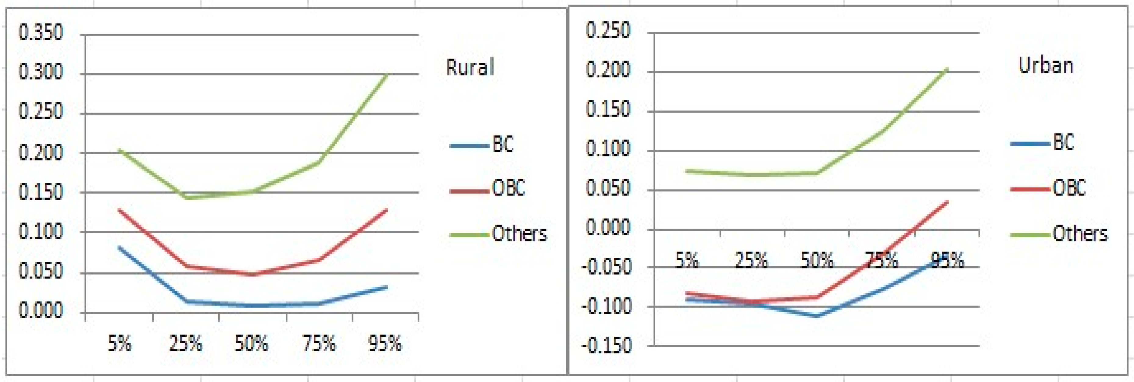
Figure 3.
Occupational types’ consumption effects for rural and urban areas for 2009–2010 (AL: Agricultural labor; OL: Other labor; SAL: Self-employed in agriculture; RW: Regular wage earner; CL: Casual labor).
Figure 3.
Occupational types’ consumption effects for rural and urban areas for 2009–2010 (AL: Agricultural labor; OL: Other labor; SAL: Self-employed in agriculture; RW: Regular wage earner; CL: Casual labor).


Table 1.
(A) Sample mean values, 1993–1994 and 1999–2000 household expenditure surveys. (B) Sample mean values, 2004–2005 and 2009–2010 household expenditure surveys.
Table 1.
(A) Sample mean values, 1993–1994 and 1999–2000 household expenditure surveys. (B) Sample mean values, 2004–2005 and 2009–2010 household expenditure surveys.
| (A) | ||||
| 1993–1994 | 1999–2000 | |||
| Variable | Rural | Urban | Rural | Urban |
| Monthly per capita consumption expenditure (Current price, Rupee) | 330.95 | 583.25 | 581.25 | 1018.76 |
| Demographic and other control variables: | ||||
| Age (years) | 44.66 | 43.23 | 45.34 | 44.14 |
| Single | 0.03 | 0.07 | 0.03 | 0.07 |
| Married | 0.86 | 0.83 | 0.86 | 0.83 |
| Divorced or widow | 0.11 | 0.10 | 0.11 | 0.10 |
| Household size | 5.15 | 4.51 | 5.25 | 4.60 |
| Male-headed | 0.91 | 0.89 | 0.90 | 0.90 |
| Social groups: | ||||
| Scheduled Tribe | 0.15 | 0.07 | 0.14 | 0.07 |
| Scheduled Caste | 0.19 | 0.11 | 0.18 | 0.12 |
| Other Backward Castes | --- | --- | 0.35 | 0.28 |
| Others | 0.66 | 0.82 | 0.33 | 0.53 |
| Occupations: | ||||
| Self-employed | --- | 0.35 | --- | 0.36 |
| Regular wage-earner | --- | 0.43 | --- | 0.42 |
| Casual labor | --- | 0.12 | --- | 0.12 |
| Self-employed in non-agriculture | 0.12 | --- | 0.15 | --- |
| Agricultural labor | 0.24 | --- | 0.26 | --- |
| Other labor | 0.07 | --- | 0.08 | --- |
| Self-employed in agriculture | 0.42 | --- | 0.38 | --- |
| Others | 0.14 | 0.10 | 0.14 | 0.10 |
| Educational level: | ||||
| Not literate at all | 0.49 | 0.20 | 0.45 | 0.19 |
| Literate, below Primary | 0.16 | 0.12 | 0.16 | 0.11 |
| Literate, Primary | 0.13 | 0.13 | 0.12 | 0.12 |
| Literate, Secondary | 0.17 | 0.30 | 0.20 | 0.31 |
| Literate, higher Secondary and above | 0.06 | 0.25 | 0.07 | 0.27 |
| Number of observations | 69,120 | 46,074 | 71,044 | 48,841 |
| (B) | ||||
| 2004–2005 | 2009–2010 | |||
| Variable | Rural | Urban | Rural | Urban |
| Monthly per capita consumption expenditure (Current price, Rupee) | 696.58 | 1122.99 | 1195.25 | 1916.93 |
| Demographic and other control variables: | ||||
| Age (years) | 46.16 | 44.95 | 46.64 | 45.82 |
| Single | 0.02 | 0.06 | 0.02 | 0.06 |
| Married | 0.86 | 0.82 | 0.87 | 0.82 |
| Divorced or widow | 0.11 | 0.12 | 0.11 | 0.12 |
| Household size | 5.08 | 4.55 | 4.86 | 4.35 |
| Male-headed | 0.89 | 0.88 | 0.89 | 0.88 |
| Social groups: | ||||
| Scheduled Tribe | 0.16 | 0.08 | 0.16 | 0.08 |
| Scheduled Caste | 0.17 | 0.14 | 0.18 | 0.14 |
| Other Backward Castes | 0.38 | 0.36 | 0.38 | 0.36 |
| Others | 0.29 | 0.42 | 0.27 | 0.42 |
| Occupations: | ||||
| Self-employed | --- | 0.39 | --- | 0.37 |
| Regular wage-earner | --- | 0.39 | --- | 0.38 |
| Casual labor | --- | 0.13 | --- | 0.13 |
| Self-employed in non-agriculture | 0.22 | --- | 0.25 | --- |
| Agricultural labor | 0.15 | --- | 0.11 | --- |
| Other labor | 0.11 | --- | 0.17 | --- |
| Self-employed in agriculture | 0.35 | --- | 0.28 | --- |
| Others | 0.17 | 0.10 | 0.19 | 0.11 |
| Educational level: | ||||
| Not literate at all | 0.37 | 0.20 | 0.31 | 0.17 |
| Literate, below Primary | 0.26 | 0.21 | 0.27 | 0.19 |
| Literate, Primary | 0.16 | 0.18 | 0.16 | 0.16 |
| Literate, Secondary | 0.15 | 0.23 | 0.19 | 0.27 |
| Literate, higher Secondary and above | 0.06 | 0.18 | 0.07 | 0.22 |
| Number of observations | 79,162 | 45,251 | 59,091 | 41,714 |
Table 2.
(A) Results of ordinary least squares (OLS) estimation for 1993–1994 and 1999–2000. (B) Results of ordinary least squares (OLS) estimation for 2004–2005 and 2009–2010.
Table 2.
(A) Results of ordinary least squares (OLS) estimation for 1993–1994 and 1999–2000. (B) Results of ordinary least squares (OLS) estimation for 2004–2005 and 2009–2010.
| (A) | ||||
| 1993–1994 | 1999–2000 | |||
| Variable | Rural | Urban | Rural | Urban |
| Constant | 4.544 *** | 4.531 *** | 5.468 *** | 5.907 *** |
| Age | 0.010 *** | 0.013 *** | 0.011 *** | 0.012 *** |
| Age squared | −0.00004 *** | −0.00006 *** | −0.00006 *** | −0.00004 *** |
| Married | −0.146 *** | −0.162 *** | −0.140 *** | −0.119 *** |
| Divorced or widow | −0.172 *** | −0.248 *** | −0.171 *** | −0.170 *** |
| Household size | −0.050 *** | −0.102 *** | −0.053 *** | −0.089 *** |
| Male-headed | −0.008 | −0.043 *** | 0.002 | −0.043 *** |
| Scheduled Caste | 0.052 *** | −0.031 ** | 0.055 *** | −0.056 *** |
| Other Backward Castes | --- | --- | 0.125 *** | 0.011 |
| Others | 0.160 *** | 0.099 *** | 0.204 *** | 0.114 *** |
| Regular wage-earner | --- | 0.028 *** | --- | 0.040 *** |
| Casual labor | --- | −0.240 *** | --- | −0.228 *** |
| Agricultural labor | −0.203 *** | --- | −0.186 *** | --- |
| Other labor | −0.121 *** | --- | −0.096 *** | --- |
| Self-employed in agriculture | 0.052 *** | --- | 0.039 *** | --- |
| Others | 0.032 *** | −0.091 *** | 0.051 *** | −0.048 *** |
| Literate, below Primary | 0.126 *** | 0.126 *** | 0.082 *** | 0.110 *** |
| Literate, Primary | 0.169 *** | 0.163 *** | 0.131 *** | 0.150 *** |
| Literate, Secondary | 0.306 *** | 0.352 *** | 0.252 *** | 0.315 *** |
| Literate, higher Secondary and above | 0.553 *** | 0.736 *** | 0.480 *** | 0.648 *** |
| R-squared | 0.3444 | 0.4519 | 0.4216 | 0.4817 |
| 1993–1994 | 1999–2000 | |||
| States | Rural | Urban | Rural | Urban |
| Arunachal Pradesh | 0.157 *** | 0.007 | 0.290 *** | −0.105 *** |
| Assam | −0.101 *** | −0.010 | −0.098 *** | −0.027 |
| Bihar | −0.225 *** | −0.114 *** | −0.117 *** | −0.116 *** |
| Goa | 0.338 *** | 0.224 *** | 0.487 *** | 0.337 *** |
| Gujarat | 0.122 *** | 0.153 *** | 0.185 *** | 0.120 *** |
| Haryana | 0.259 *** | 0.120 *** | 0.348 *** | 0.201 *** |
| Himachal Pradesh | 0.109 *** | 0.259 *** | 0.258 *** | 0.283 *** |
| Jammu and Kashmir | 0.188 *** | 0.201 *** | 0.294 *** | 0.229 *** |
| Karnataka | −0.015 | 0.037 *** | 0.103 *** | 0.084 *** |
| Kerala | 0.165 *** | 0.140 *** | 0.357 *** | 0.197 *** |
| Madhya Pradesh | −0.079 *** | −0.010 | −0.058 *** | −0.067 *** |
| Maharashtra | −0.093 *** | 0.176 *** | 0.016 * | 0.151 *** |
| Manipur | −0.001 | −0.231 *** | 0.074 *** | −0.144 *** |
| Meghalaya | 0.234 *** | 0.183 *** | 0.297 *** | 0.230 *** |
| Mizoram | 0.316 *** | 0.357 *** | 0.418 *** | 0.361 *** |
| Nagaland | 0.430 *** | 0.281 *** | 0.718 *** | 0.449 *** |
| Orissa | −0.208 *** | −0.038 ** | −0.174 *** | −0.112 *** |
| Punjab | 0.412 *** | 0.261 *** | 0.449 *** | 0.199 *** |
| Rajasthan | 0.129 *** | 0.067 *** | 0.220 *** | 0.074 *** |
| Sikkim | −0.004 | 0.189 *** | 0.107 *** | 0.212 *** |
| Tamil Nadu | −0.040 *** | −0.026 ** | 0.075 *** | 0.065 *** |
| Tripura | 0.095 *** | 0.098 *** | 0.079 *** | 0.097 *** |
| Uttar Pradesh | −0.061 *** | −0.019 * | 0.000 | −0.042 *** |
| West Bengal | −0.014 | 0.025 ** | −0.004 | −0.025 ** |
| A and N Islands | 0.553 *** | 0.615 *** | 0.503 *** | 0.371 *** |
| Chandigarh | 0.469 *** | 0.479 *** | 0.623 *** | 0.429 *** |
| Dadra and Nagar Haveli | −0.001 | 0.090 | 0.226 *** | 0.244 *** |
| Daman and Diu | 0.497 *** | 0.219 *** | 0.646 *** | 0.211 *** |
| Delhi | 0.610 *** | 0.419 *** | 0.530 *** | 0.338 *** |
| Lakshdweep | 0.711 *** | 0.428 *** | 0.724 *** | 0.622 *** |
| Pondicherry | 0.264 *** | 0.019 | 0.252 *** | 0.081 *** |
| (B) | ||||
| 2004–2005 | 2009–2010 | |||
| Variable | Rural | Urban | Rural | Urban |
| Constant | 5.775 *** | 6.103 *** | 6.835 *** | 7.234 *** |
| Age | 0.018 *** | 0.021 *** | 0.015 *** | 0.009 *** |
| Age squared | −0.00012 *** | −0.00014 *** | −0.00009 *** | −0.00003 ** |
| Married | −0.110 *** | −0.148 *** | −0.184 *** | −0.235 *** |
| Divorced or widow | −0.149 *** | −0.214 *** | −0.214 *** | −0.292 *** |
| Household size | −0.051 *** | −0.089 *** | −0.061 *** | −0.094 *** |
| Male-headed | −0.023 *** | −0.020 * | −0.010 | −0.044 *** |
| Scheduled Caste | 0.044 *** | −0.034 *** | 0.040 *** | −0.050 *** |
| Other Backward Castes | 0.132 *** | 0.009 | 0.112 *** | −0.003 |
| Others | 0.192 *** | 0.154 *** | 0.183 *** | 0.127 *** |
| Regular wage-earner | --- | 0.037 *** | --- | 0.059 *** |
| Casual labor | --- | −0.225 *** | --- | −0.255 *** |
| Agricultural labor | −0.191 *** | --- | −0.196 *** | --- |
| Other labor | −0.110 *** | --- | −0.121 *** | --- |
| Self-employed in agriculture | 0.051 *** | --- | 0.081 *** | --- |
| Others | 0.056 *** | −0.005 | 0.086 *** | −0.008 |
| Literate, below Primary | 0.118 *** | 0.127 *** | 0.107 *** | 0.129 *** |
| Literate, Primary | 0.229 *** | 0.263 *** | 0.212 *** | 0.258 *** |
| Literate, Secondary | 0.364 *** | 0.471 *** | 0.340 *** | 0.471 *** |
| Literate, higher Secondary and above | 0.599 *** | 0.821 *** | 0.543 *** | 0.782 *** |
| R-squared | 0.3927 | 0.4741 | 0.4439 | 0.5085 |
| 2004–2005 | 2009–2010 | |||
| States | Rural | Urban | Rural | Urban |
| Arunachal Pradesh | 0.286 *** | −0.042 * | 0.149 *** | −0.186 *** |
| Assam | −0.085 *** | −0.042 ** | −0.251 *** | −0.330 *** |
| Bihar | −0.253 *** | −0.235 *** | −0.316 *** | −0.381 *** |
| Goa | 0.316 *** | 0.221 *** | 0.387 *** | 0.162 *** |
| Gujarat | 0.065 *** | 0.122 *** | 0.045 *** | −0.035 ** |
| Haryana | 0.252 *** | 0.184 *** | 0.238 *** | 0.089 *** |
| Himachal Pradesh | 0.161 *** | 0.268 *** | 0.145 *** | 0.082 *** |
| Jammu and Kashmir | 0.241 *** | 0.198 *** | 0.068 *** | −0.145 *** |
| Karnataka | −0.125 *** | 0.024 * | −0.124 *** | −0.110 *** |
| Kerala | 0.341 *** | 0.233 *** | 0.313 *** | 0.114 *** |
| Madhya Pradesh | −0.183 *** | −0.076 *** | −0.218 *** | −0.251 *** |
| Maharashtra | −0.088 *** | 0.142 *** | −0.047 *** | 0.003 |
| Manipur | −0.031 *** | −0.128 *** | −0.199 *** | −0.523 *** |
| Meghalaya | 0.244 *** | 0.209 *** | 0.028 * | −0.061 ** |
| Mizoram | 0.354 *** | 0.392 *** | 0.122 *** | 0.080 *** |
| Nagaland | 0.504 *** | 0.438 *** | 0.258 *** | −0.007 |
| Orissa | −0.357 *** | −0.216 *** | −0.390 *** | −0.334 *** |
| Punjab | 0.358 *** | 0.226 *** | 0.339 *** | 0.062 *** |
| Rajasthan | 0.074 *** | 0.108 *** | 0.067 *** | 0.006 |
| Sikkim | 0.114 *** | 0.043 | 0.110 *** | 0.181 *** |
| Tamil Nadu | −0.031 *** | 0.064 *** | −0.059 *** | −0.089 *** |
| Tripura | −0.160 *** | −0.024 | −0.036 *** | −0.125 *** |
| Uttar Pradesh | −0.072 *** | −0.038 *** | −0.189 *** | −0.217 *** |
| West Bengal | −0.038 *** | 0.008 | −0.183 *** | −0.217 *** |
| A and N Islands | 0.370 *** | 0.510 *** | 0.399 *** | 0.449 *** |
| Chandigarh | 0.383 *** | 0.293 *** | 0.531 *** | 0.334 *** |
| Dadra and Nagar Haveli | 0.068 ** | 0.225 *** | −0.014 | 0.045 |
| Daman and Diu | 0.602 *** | 0.394 *** | 0.277 *** | 0.059 *** |
| Delhi | 0.380 *** | 0.304 *** | 0.337 *** | 0.170 *** |
| Lakshdweep | 0.623 *** | 0.646 *** | 0.477 *** | 0.546 *** |
| Pondicherry | 0.193 *** | 0.126 *** | 0.347 *** | 0.225 *** |
| Chattigarh | −0.223 *** | −0.094 *** | −0.314 *** | −0.308 *** |
| Jharkhand | −0.223 *** | −0.033 * | −0.302 *** | −0.266 *** |
| Uttaranchal | −0.035 *** | 0.053 *** | −0.033 ** | −0.101 *** |
Notes: * Significant at 10% level; ** Significant at 5% level; *** Significant at 1% level. Reference characteristics: Female-headed, Single, Other castes, Self-employed, Not literate, and state of Andhra Pradesh.
Table 3.
(A) Results of quantile regressions for 1993–1994. (B) Results of quantile regressions for 1999–2000. (C) Results of quantile regressions for 2004–2005. (D) Results of quantile regressions for 2009–2010.
Table 3.
(A) Results of quantile regressions for 1993–1994. (B) Results of quantile regressions for 1999–2000. (C) Results of quantile regressions for 2004–2005. (D) Results of quantile regressions for 2009–2010.
| (A) | ||||||||||
| 1993–1994 (50th) | Q5 | Q25 | Q50 | Q75 | Q95 | |||||
| Rural | Urban | Rural | Urban | Rural | Urban | Rural | Urban | Rural | Urban | |
| Constant | 3.671 *** | 3.843 *** | 4.251 *** | 4.406 *** | 4.636 *** | 4.770 *** | 5.035 *** | 5.124 *** | 5.484 *** | 5.718 *** |
| Age | 0.013 *** | 0.014 *** | 0.011 *** | 0.014 *** | 0.007 *** | 0.012 *** | 0.006 *** | 0.011 *** | 0.007 *** | 0.006 *** |
| Age squared | −0.0001 *** | −0.0001 *** | −0.0001 *** | −0.0001 *** | −0.00001 *** | −0.0001 *** | 0.00001 | −0.00002 | −0.00001 | 0.00005 |
| Married | −0.026 | −0.047 * | −0.111 *** | −0.157 *** | −0.133 *** | −0.202 *** | −0.183 *** | −0.220 *** | −0.246 *** | −0.214 *** |
| Divorced or widow | −0.086 *** | −0.142 *** | −0.148 *** | −0.233 *** | −0.165 *** | −0.287 *** | −0.209 *** | −0.325 *** | −0.211 *** | −0.336 *** |
| Household size | −0.045 *** | −0.087 *** | −0.050 *** | −0.103 *** | −0.052 *** | −0.109 *** | −0.054 *** | −0.113 *** | −0.054 *** | −0.108 *** |
| Male-headed | 0.025 | 0.005 | −0.010 | −0.021 | −0.033 *** | −0.052 *** | −0.067 *** | −0.096 *** | −0.043 *** | −0.158 *** |
| Scheduled Caste | 0.041 *** | −0.172 *** | 0.004 *** | −0.177 *** | −0.002 *** | −0.147 *** | −0.007 | −0.113 *** | −0.010 *** | −0.065 ** |
| Others | 0.116 *** | −0.050 *** | 0.079 *** | −0.066 *** | 0.079 *** | −0.047 *** | 0.087 *** | 0.001 | 0.130 *** | 0.046 ** |
| Regular wage-earner | --- | 0.075 *** | --- | 0.067 *** | --- | 0.046 *** | --- | 0.014 | --- | −0.051 *** |
| Casual labor | --- | −0.184 *** | --- | −0.203 *** | --- | −0.241 *** | --- | −0.278 *** | --- | −0.350 *** |
| Agricultural labor | −0.187 *** | --- | −0.217 *** | --- | −0.240 *** | --- | −0.273 *** | --- | −0.293 *** | --- |
| Other labor | −0.041 *** | --- | −0.071 *** | --- | −0.083 *** | --- | −0.102 *** | --- | −0.108 *** | --- |
| Self-employed in agriculture | 0.041 *** | --- | 0.047 *** | --- | 0.043 *** | --- | 0.035 *** | --- | 0.078 *** | --- |
| Others | −0.011 | −0.158 *** | 0.051 *** | −0.108 *** | 0.060 *** | −0.091 *** | 0.066 *** | −0.073 *** | 0.102 *** | −0.092 *** |
| Literate, below Primary | 0.140 *** | 0.133 *** | 0.136 *** | 0.147 *** | 0.123 *** | 0.136 *** | 0.114 *** | 0.116 *** | 0.120 *** | 0.143 *** |
| Literate, Primary | 0.185 *** | 0.177 *** | 0.191 *** | 0.201 *** | 0.206 *** | 0.191 *** | 0.213 *** | 0.192 *** | 0.224 *** | 0.214 *** |
| Literate, Secondary | 0.272 *** | 0.319 *** | 0.290 *** | 0.343 *** | 0.314 *** | 0.367 *** | 0.346 *** | 0.389 *** | 0.424 *** | 0.473 *** |
| Literate, higher Secondary and above | 0.491 *** | 0.585 *** | 0.492 *** | 0.664 *** | 0.542 *** | 0.740 *** | 0.598 *** | 0.825 *** | 0.669 *** | 0.877 *** |
| Spatial fixed effects included | ||||||||||
| Pseudo R-squared | 0.109 | 0.180 | 0.135 | 0.229 | 0.147 | 0.257 | 0.157 | 0.271 | 0.163 | 0.244 |
| (B) | ||||||||||
| 1999–2000 (55th) | Q5 | Q25 | Q50 | Q75 | Q95 | |||||
| Rural | Urban | Rural | Urban | Rural | Urban | Rural | Urban | Rural | Urban | |
| Constant | 4.632 *** | 5.187 *** | 5.204 *** | 5.768 *** | 5.615 *** | 6.140 *** | 5.975 *** | 6.498 *** | 6.593 *** | 7.028 *** |
| Age | 0.019 *** | 0.014 *** | 0.012 *** | 0.013 *** | 0.010 *** | 0.010 *** | 0.009 *** | 0.008 *** | 0.006 *** | 0.005 *** |
| Age squared | −0.00014 *** | −0.0001 *** | −0.0001 *** | −0.0001 *** | −0.00004 *** | −0.00003 ** | −0.00002 | 0.00001 | 0.00002 | 0.00005 ** |
| Married | −0.036 | −0.016 | −0.093 *** | −0.116 *** | −0.153 *** | −0.122 *** | −0.192 *** | −0.155 *** | −0.267 *** | −0.180 *** |
| Divorced or widow | −0.097 *** | −0.069 *** | −0.129 *** | −0.182 *** | −0.182 *** | −0.196 *** | −0.219 *** | −0.213 *** | −0.317 *** | −0.250 *** |
| Household size | −0.049 *** | −0.083 *** | −0.053 *** | −0.094 *** | −0.055 *** | −0.097 *** | −0.056 *** | −0.095 *** | −0.057 *** | −0.089 *** |
| Male-headed | 0.003 | 0.002 | 0.0001 | −0.041 *** | −0.033 *** | −0.078 *** | −0.054 *** | −0.087 *** | −0.086 *** | −0.142 *** |
| Scheduled Caste | 0.047 *** | −0.108 *** | 0.036 *** | −0.156 *** | 0.0001 | −0.174 *** | −0.011 | −0.175 *** | −0.026 | −0.143 *** |
| Other Backward Castes | 0.100 *** | −0.060 *** | 0.079 *** | −0.110 *** | 0.040 *** | −0.131 *** | 0.032 *** | −0.144 *** | 0.013 | −0.117 *** |
| Others | 0.206 *** | 0.054 *** | 0.194 *** | 0.010 | 0.159 *** | 0.001 | 0.155 *** | 0.001 | 0.136 *** | 0.043 * |
| Regular wage-earner | --- | 0.100 *** | --- | 0.088 *** | --- | 0.075 *** | --- | 0.034 *** | --- | −0.003 |
| Casual labor | --- | −0.182 *** | --- | −0.191 *** | --- | −0.215 *** | --- | −0.244 *** | --- | −0.286 *** |
| Agricultural labor | −0.156 *** | --- | −0.175 *** | --- | −0.209 *** | --- | −0.248 *** | --- | −0.323 *** | --- |
| Other labor | −0.056 *** | --- | −0.033 *** | --- | −0.034 *** | --- | −0.052 *** | --- | −0.072 *** | --- |
| Self-employed in agriculture | 0.045 *** | --- | 0.048 *** | --- | 0.047 *** | --- | 0.035 *** | --- | 0.022 *** | --- |
| Others | 0.005 | −0.091 *** | 0.074 *** | −0.079 *** | 0.104 *** | −0.064 *** | 0.101 *** | −0.063 *** | 0.084 *** | −0.039 ** |
| Literate, below Primary | 0.093 *** | 0.122 *** | 0.089 *** | 0.117 *** | 0.088 *** | 0.116 *** | 0.097 *** | 0.130 *** | 0.101 *** | 0.155 *** |
| Literate, Primary | 0.148 *** | 0.162 *** | 0.156 *** | 0.190 *** | 0.166 *** | 0.191 *** | 0.179 *** | 0.205 *** | 0.201 *** | 0.190 *** |
| Literate, Secondary | 0.217 *** | 0.299 *** | 0.239 *** | 0.329 *** | 0.272 *** | 0.349 *** | 0.314 *** | 0.375 *** | 0.373 *** | 0.382 *** |
| Literate, higher Secondary and above | 0.373 *** | 0.538 *** | 0.410 *** | 0.614 *** | 0.482 *** | 0.653 *** | 0.551 *** | 0.707 *** | 0.670 *** | 0.768 *** |
| Spatial fixed effects included | ||||||||||
| Pseudo R-squared | 0.120 | 0.207 | 0.153 | 0.260 | 0.173 | 0.276 | 0.192 | 0.271 | 0.214 | 0.242 |
| (C) | ||||||||||
| 2003–2004 (61st) | Q5 | Q25 | Q50 | Q75 | Q95 | |||||
| Rural | Urban | Rural | Urban | Rural | Urban | Rural | Urban | Rural | Urban | |
| Constant | 4.234 *** | 4.904 *** | 5.147 *** | 5.730 *** | 5.656 *** | 6.192 *** | 6.075 *** | 6.673 *** | 6.716 *** | 7.279 *** |
| Age | 0.030 *** | 0.030 *** | 0.021 *** | 0.024 *** | 0.016 *** | 0.019 *** | 0.014 *** | 0.014 *** | 0.012 *** | 0.009 *** |
| Age squared | −0.00025 *** | −0.00025 *** | −0.00015 *** | −0.00017 *** | −0.00009 *** | −0.00011 *** | −0.00006 *** | −0.00005 *** | −0.00003 | 0.00001 |
| Married | 0.170 *** | 0.008 | −0.094 *** | −0.145 *** | −0.152 *** | −0.175 *** | −0.218 *** | −0.238 *** | −0.296 *** | −0.271 *** |
| Divorced or widow | 0.106 | −0.071 | −0.129 *** | −0.238 *** | −0.192 *** | −0.269 *** | −0.253 *** | −0.311 *** | −0.361 *** | −0.361 *** |
| Household size | −0.048 *** | −0.068 *** | −0.052 *** | −0.088 *** | −0.054 *** | −0.096 *** | −0.056 *** | −0.098 *** | −0.058 *** | −0.091 *** |
| Male-headed | 0.030 ** | 0.019 | −0.007 | −0.027 * | −0.052 *** | −0.068 *** | −0.077 *** | −0.081 *** | −0.176 *** | −0.148 *** |
| Scheduled Caste | 0.079 *** | −0.101 *** | −0.001 | −0.172 *** | −0.038 *** | −0.167 *** | −0.046 *** | −0.171 *** | −0.011 *** | −0.123 *** |
| Other Backward Castes | 0.129 *** | −0.104 *** | 0.043 *** | −0.165 *** | 0.013 ** | −0.161 *** | 0.018 *** | −0.153 *** | 0.094 *** | −0.103 *** |
| Others | 0.231 *** | 0.051 *** | 0.146 *** | 0.011 | 0.124 *** | 0.025 * | 0.137 *** | 0.044 *** | 0.209 *** | 0.102 *** |
| Regular wage-earner | --- | 0.085 *** | --- | 0.071 *** | --- | 0.068 *** | --- | 0.045 *** | --- | 0.019 |
| Casual labor | --- | −0.132 *** | --- | −0.171 *** | --- | −0.204 *** | --- | −0.254 *** | --- | −0.306 *** |
| Agricultural labor | −0.124 *** | --- | −0.164 *** | --- | −0.197 *** | --- | −0.234 *** | --- | −0.305 *** | --- |
| Other labor | −0.039 *** | --- | −0.037 *** | --- | −0.054 *** | --- | −0.078 *** | --- | −0.107 *** | --- |
| Self-employed in agriculture | 0.082 *** | --- | 0.084 *** | --- | 0.078 *** | --- | 0.059 *** | --- | 0.051 *** | --- |
| Others | 0.059 *** | −0.077 *** | 0.093 *** | −0.052 *** | 0.110 *** | −0.014 | 0.103 *** | 0.001 | 0.045 *** | 0.011 |
| Literate, below Primary | 0.131 *** | 0.132 *** | 0.141 *** | 0.127 *** | 0.128 *** | 0.153 *** | 0.129 *** | 0.172 *** | 0.141 *** | 0.187 *** |
| Literate, Primary | 0.224 *** | 0.236 *** | 0.240 *** | 0.262 *** | 0.239 *** | 0.307 *** | 0.257 *** | 0.323 *** | 0.307 *** | 0.346 *** |
| Literate, Secondary | 0.327 *** | 0.357 *** | 0.360 *** | 0.454 *** | 0.375 *** | 0.519 *** | 0.411 *** | 0.542 *** | 0.506 *** | 0.568 *** |
| Literate, higher Secondary and above | 0.516 *** | 0.661 *** | 0.561 *** | 0.799 *** | 0.596 *** | 0.838 *** | 0.654 *** | 0.874 *** | 0.842 *** | 0.955 *** |
| Spatial fixed effects are included | ||||||||||
| Pseudo R-squared | 0.129 | 0.165 | 0.149 | 0.238 | 0.161 | 0.283 | 0.172 | 0.286 | 0.163 | 0.253 |
| (D) | ||||||||||
| 2009–2010 (66th) | Q5 | Q25 | Q50 | Q75 | Q95 | |||||
| Rural | Urban | Rural | Urban | Rural | Urban | Rural | Urban | Rural | Urban | |
| Constant | 5.712 *** | 6.284 *** | 6.301 *** | 7.039 *** | 6.703 *** | 7.433 *** | 7.083 *** | 7.724 *** | 7.746 *** | 8.292 *** |
| Age | 0.017 *** | 0.014 *** | 0.016 *** | 0.007 *** | 0.013 *** | 0.007 *** | 0.015 *** | 0.008 *** | 0.013 *** | 0.003 * |
| Age squared | −0.0001 *** | −0.0001 *** | −0.0001 *** | −0.00001 *** | −0.0001 *** | 0.00001 *** | −0.0001 *** | 0.00001 | −0.00003 | 0.0001 *** |
| Married | 0.016 | −0.106 *** | −0.081 *** | −0.193 *** | −0.162 *** | −0.226 *** | −0.298 *** | −0.278 *** | −0.499 *** | −0.365 *** |
| Divorced or widow | −0.032 | −0.231 *** | −0.124 *** | −0.291 *** | −0.197 *** | −0.328 *** | −0.333 *** | −0.361 *** | −0.552 *** | −0.399 *** |
| Household size | −0.056 *** | −0.090 *** | −0.063 *** | −0.104 *** | −0.066 *** | −0.108 *** | −0.069 *** | −0.107 *** | −0.071 *** | −0.095 *** |
| Male-headed | 0.022 | 0.034 * | −0.027 *** | −0.029 | −0.047 *** | −0.093 *** | −0.067 *** | −0.125 *** | −0.137 *** | −0.148 *** |
| Scheduled Caste | 0.082 *** | −0.090 *** | 0.013 ** | −0.096 *** | 0.007 | −0.112 *** | 0.010 | −0.077 *** | 0.031 *** | −0.034 |
| Other Backward Castes | 0.130 *** | −0.081 *** | 0.057 *** | −0.093 *** | 0.047 *** | −0.088 *** | 0.066 *** | −0.032 *** | 0.130 *** | 0.033 *** |
| Others | 0.205 *** | 0.075 *** | 0.145 *** | 0.069 *** | 0.152 *** | 0.071 *** | 0.190 *** | 0.123 *** | 0.299 *** | 0.202 *** |
| Regular wage-earner | --- | 0.135 *** | --- | 0.128 *** | --- | 0.105 *** | --- | 0.084 *** | --- | 0.041 *** |
| Casual labor | --- | −0.122 *** | --- | −0.201 *** | --- | −0.234 *** | --- | −0.250 *** | --- | −0.312 *** |
| Agricultural labor | −0.167 *** | --- | −0.156 *** | --- | −0.174 *** | --- | −0.206 *** | --- | −0.228 *** | --- |
| Other labor | −0.043 *** | --- | −0.036 *** | --- | −0.054 *** | --- | −0.076 *** | --- | −0.101 *** | --- |
| Self-employed in agriculture | 0.099 *** | --- | 0.100 *** | --- | 0.096 *** | --- | 0.086 *** | --- | 0.119 *** | --- |
| Others | 0.098 *** | −0.108 *** | 0.133 *** | −0.055 *** | 0.151 *** | −0.020 | 0.147 *** | 0.010 | 0.143 *** | 0.086 *** |
| Literate, below Primary | 0.142 *** | 0.095 *** | 0.125 *** | 0.124 *** | 0.125 *** | 0.138 *** | 0.136 *** | 0.159 *** | 0.153 *** | 0.174 *** |
| Literate, Primary | 0.240 *** | 0.223 *** | 0.234 *** | 0.247 *** | 0.231 *** | 0.274 *** | 0.255 *** | 0.298 *** | 0.274 *** | 0.304 *** |
| Literate, Secondary | 0.341 *** | 0.387 *** | 0.341 *** | 0.438 *** | 0.352 *** | 0.463 *** | 0.377 *** | 0.490 *** | 0.447 *** | 0.492 *** |
| Literate, higher Secondary and above | 0.506 *** | 0.679 *** | 0.509 *** | 0.708 *** | 0.540 *** | 0.738 *** | 0.596 *** | 0.781 *** | 0.718 *** | 0.845 *** |
| Spatial fixed effects are included | ||||||||||
| Pseudo R-squared | 0.143 | 0.195 | 0.159 | 0.262 | 0.172 | 0.282 | 0.190 | 0.274 | 0.199 | 0.260 |
Note: * Significant at 10% level; ** Significant at 5% level; *** Significant at 1% level.
Table 4.
(A) Results of poverty dominance (report on the first intersection between two distributions). (B) Results of poverty dominance (report on the last intersection between two distributions). (C) Results of poverty dominance (report on full dominance only).
Table 4.
(A) Results of poverty dominance (report on the first intersection between two distributions). (B) Results of poverty dominance (report on the last intersection between two distributions). (C) Results of poverty dominance (report on full dominance only).
| (A) | ||||||
| First-Order Dominance | Second-Order Dominance | Third-Order Dominance | ||||
| Pair Comparison | Rural | Urban | Rural | Urban | Rural | Urban |
| 66 vs. 61 | B (2.50) | C | A (5.30) * | C | B (4.29) | C |
| 66 vs. 55 | A (7.16) * | C | A (12.94) * | C | A (18.56) * | C |
| 66 vs. 50 | C | C | C | C | C | C |
| 61 vs. 55 | A (58.51) | A (89.09) | A (82.58) * | A (113.58) * | A (100.14) * | A (137.83) * |
| 61 vs. 50 | C | C | C | C | C | C |
| 55 vs. 50 | C | C | C | C | C | C |
| 50th | ||||||
| BC vs. OTH | B (1.77) | A (14.69) | B (2.42) * | D | B (3.23) * | D |
| MHHs vs. FHHs | A (3.23) | B (384.75) | A (8.03) | C | A (9.74) | C |
| T1 vs. T2 | B (2.36) | B (9.65) * | B (3.95) | B (12.18) | B (6.24) | B (15.32) * |
| T1 vs. T3 | B (2.34) | A (19.13) * | B (2.46) | A (25.77) * | B (2.68) | A (31.90) * |
| T1 vs. T4 | A (6.04) | B (60.33) | A (9.37) | B (78.20) * | A (12.42) | B (98.65) * |
| T2 vs. T3 | D | A (14.69) * | D | A (18.11) * | D | A (22.30) * |
| T2 vs. T4 | A (3.23) | B (203.39) | A (6.63) | B (523.27) * | A (10.19) | D |
| T3 vs. T4 | A (2.38) | B (35.79) * | B (102.11) * | B (47.76) * | A (3.12) | B (59.32) * |
| 55th | ||||||
| BC vs. OTH | D | A (23,931.58) * | D | D | D | D |
| MHHs vs. FHHs | A (26.87) | A (35.40) | A (36.33) | A (54.42) | A (45.64) | A (72.80) |
| T1 vs. T2 | A (50.75) | B (83.19) | A (61.72) * | B (106.52) * | A (73.44) * | B (127.51) * |
| T1 vs. T3 | A (371.33) | A (53.10) | A (1012.84) * | A (61.75) * | C | A (72.58) * |
| T1 vs. T4 | B (151.04) | B (158.71) | B (189.26) * | B (205.62) * | B (230.31) * | B (250.85) * |
| T2 vs. T3 | A (5904.93) | A (59.00) | D | A (76.08) * | D | A (95.20) * |
| T2 vs. T4 | B (74.63) * | B (682.63) * | A (96.56) * | B (1430.94) * | B (11.4.48) * | D |
| T3 vs. T4 | B (197.01) | B (102.66) | B (248.16) * | B (127.57) * | B (304.85) * | B (150.16) * |
| 61st | ||||||
| BC vs. OTH | B (9.27) * | A (14.38) | B (16.16) * | A (57.48) | B (22.30) * | D |
| MHHs vs. FHHs | B (250.37) | B (2345.20) | B (326.97) * | C | B (427.27) * | C |
| T1 vs. T2 | A (61.20) * | B (153.93) * | A (73.31) * | B (178.68) * | A (83.64) * | B (206.66) * |
| T1 vs. T3 | A (70.74) | B (16,000) | D | C | D | C |
| T1 vs. T4 | B (166.16) | B (229.96) | B (223.22) * | B (315.52) * | B (276.75) * | B (403.99) * |
| T2 vs. T3 | --- | A (71.33) | D | A (97.61) * | D | A (114.43) * |
| T2 vs. T4 | B (97.98) | B (721.36) | B (126.74) * | B (1284.72) * | B (133.26) * | D |
| T3 vs. T4 | B (317.60) | B (158.61) * | B (433.84) * | B (205.97) * | B (568.70) * | B (256.78) * |
| 66th | ||||||
| BC vs. OTH | A (74.00) | D | --- | D | D | D |
| MHHs vs. FHHs | A (62.00) | B (1976.00) | B (561.74) * | B (5661.63) * | A (94.43) | B (11983.33) * |
| T1 vs. T2 | --- | --- | C | D | C | D |
| T1 vs. T3 | B (197.87) | A (168.00) | B (266.516) * | A (191.66) * | B (295.07) | C |
| T1 vs. T4 | B (279.86) | B (400.00) | B (482.91) * | B (467,79) * | B (556.61) | B (567.09) * |
| T2 vs. T3 | D | A (168.00) * | D | A (178.22) * | D | A (197.65) * |
| T2 vs. T4 | B (144.71) * | B (1815.60) | B (169.93) * | B (3256.94) * | B (204.67) | B (5263.05) * |
| T3 vs. T4 | B (874.80) | B (248.44) | B (1334.464) * | B (302.50) * | B (1915.79) | B (355.10) * |
| (B) | ||||||
| First-Order Dominance | Second-Order Dominance | Third-Order Dominance | ||||
| Pair comparison | Rural | Urban | Rural | Urban | Rural | Urban |
| 66 vs.61 | A (4.63) | C | A (5.30) * | C | A (6.22) | C |
| 66 vs.55 | A (7.16) * | C | A (12.94) * | C | A (18.56) * | C |
| 66 vs.50 | C | C | C | C | C | C |
| 61 vs.55 | A (59.70) | B (104,104.24) | A (82.58) * | A (113.58) * | A (100.14) * | A (137.83) * |
| 61 vs.50 | C | C | C | C | C | C |
| 55 vs.50 | C | C | C | C | C | C |
| 50th | ||||||
| BC vs. OTH | A (7735.91) | B (22.13) | B (2.42) * | D | B (3.23) * | D |
| MHHs vs. FHHs | A (1918.48) | A (7250.99) | B (74.92) | C | B (94.43) | C |
| T1 vs. T2 | A (15.08) | B (9.65) * | A (17.11) | B (12.18) * | A (21.53) | B (15.32) * |
| T1 vs. T3 | B (1180.41) | A (19.13) * | B (8853.240) | A (25.77) * | A (308.62) | A (31.90) * |
| T1 vs. T4 | B (1175.13) | B (62.07) | B (74.57) | B (78.20) * | B (88.68) | B (98.65) * |
| T2 vs. T3 | D | A (14.69) * | D | A (18.11) * | D | A (22.30) * |
| T2 vs. T4 | B (20.60) | A (13,642.43) | B (25.51) | B (523.27) * | B (30.96) | D |
| T3 vs. T4 | A (2216.04) | B (35.79) * | B (102.11) * | B (47.76) * | B (127.87) | B (59.32) |
| 55th | ||||||
| BC vs. OTH | D | A (23,931.58) | D | D | D | D |
| MHHs vs. FHHs | B (139.70) | A (21,011.08) | B (168.00) | B (1329.87) | B (204.54) | B (2090.55) |
| T1 vs. T2 | B (10,006.92) | A (8035.21) | A (61.72) * | B (106.52) * | A (73.44) * | B (127.51) * |
| T1 vs. T3 | B (10,006.92) | B (28,911.52) | A (1012.84) * | A (61.75) * | C | A (72.58) * |
| T1 vs. T4 | B (10,006.92) | A (49,810.16) | B (189.26) * | B (205.62) * | B (230.31) * | B (250.85) * |
| T2 vs. T3 | B (11,023.61) | B (8934.00) | D | A (76.08) * | D | A (95.20) * |
| T2 vs. T4 | B (74.63) * | B (682.63) * | A (96.56) * | B (1430.94) * | B (11.4.48) * | D |
| T3 vs. T4 | A (15,789.47) | A (49,810.16) | B (248.16) * | B (127.57) * | B (304.85) * | B (150.16) * |
| 61st | ||||||
| BC vs. OTH | B (9.27) * | B (71.18) | B (16.16) * | B (88.09) | B (22.30) * | D |
| MHHs vs. FHHs | A (34401.69) | A (4124.65) | B (326.97) * | C | B (427.27) * | C |
| T1 vs. T2 | A (61.20) * | B (153.93) * | A (73.31) * | B (178.68) * | A (83.64) * | B (206.66) * |
| T1 vs. T3 | A (39,854.19) | A (27,578.41) | D | C | D | C |
| T1 vs. T4 | A (34,567.16) | B (231.52) | B (223.22) * | B (315.52) * | B (276.75) * | B (403.99) * |
| T2 vs. T3 | --- | A (27,578.41) | D | A (97.61) * | D | A (114.43) * |
| T2 vs. T4 | B (97.98) | B (41753.77) | B (126.74) * | B (1284.72) * | B (133.26) * | D |
| T3 vs. T4 | A (54,119.16) | B (158.61) * | B (433.84) * | B (205.97) * | B (568.70) * | B (256.78) * |
| 66th | ||||||
| BC vs. OTH | B (117.00) | D | --- | D | D | D |
| MHHs vs. FHHs | A (124,470.33) | A (11,918.00) | B (561.74) * | B (5661.63) * | B (697.58) | B (11,983.33) * |
| T1 vs. T2 | --- | --- | C | D | C | D |
| T1 vs. T3 | B (132,960.50) | A (245.14) | B (266.516) * | A (191.66) * | B (295.07) | C |
| T1 vs. T4 | B (132,960.50) | B (71,870.20) | B (482.91) * | B (467,79) * | B (556.61) | B (567.09) * |
| T2 vs. T3 | D | A (168.00) * | D | A (178.22) * | D | A (197.65) * |
| T2 vs. T4 | B (144.71) * | B (132,201.50) | B (169.93) * | B (3256.94) * | B (204.67) | B (5263.05) * |
| T3 vs. T4 | A (124,470.33) | B (254.17) | B (1334.464) * | B (302.50) * | B (1915.79) | B (355.10) * |
| (C) | ||||||
| First-Order Dominance | Second-Order Dominance | Third-Order Dominance | ||||
| Pair comparison | Rural | Urban | Rural | Urban | Rural | Urban |
| 66 vs. 61 | --- | C | --- | C | --- | C |
| 66 vs. 55 | --- | C | --- | C | --- | C |
| 66 vs. 50 | C | C | C | C | C | C |
| 61 vs. 55 | --- | --- | --- | --- | --- | --- |
| 61 vs. 50 | C | C | C | C | C | C |
| 55 vs. 50 | C | C | C | C | C | C |
| 50th | ||||||
| BC vs. OTH | --- | --- | --- | D | --- | D |
| MHHs vs. FHHs | --- | --- | --- | C | --- | C |
| T1 vs. T2 | --- | --- | --- | --- | --- | --- |
| T1 vs. T3 | --- | --- | --- | --- | --- | --- |
| T1 vs. T4 | --- | --- | --- | --- | --- | --- |
| T2 vs. T3 | D | --- | D | --- | D | --- |
| T2 vs. T4 | --- | --- | --- | --- | --- | D |
| T3 vs. T4 | --- | --- | --- | --- | --- | --- |
| 55th | ||||||
| BC vs. OTH | D | --- | D | D | D | D |
| MHHs vs. FHHs | --- | --- | --- | --- | --- | --- |
| T1 vs. T2 | --- | --- | --- | --- | --- | --- |
| T1 vs. T3 | --- | --- | --- | --- | C | --- |
| T1 vs. T4 | --- | --- | --- | --- | --- | --- |
| T2 vs. T3 | --- | --- | D | --- | D | --- |
| T2 vs. T4 | --- | --- | --- | --- | --- | D |
| T3 vs. T4 | --- | --- | --- | --- | --- | --- |
| 61st | ||||||
| BC vs. OTH | --- | --- | --- | --- | --- | D |
| MHHs vs. FHHs | --- | --- | --- | C | --- | C |
| T1 vs. T2 | --- | --- | --- | --- | --- | --- |
| T1 vs. T3 | --- | --- | D | C | D | C |
| T1 vs. T4 | --- | --- | --- | --- | --- | --- |
| T2 vs. T3 | --- | --- | D | --- | D | --- |
| T2 vs. T4 | --- | --- | --- | --- | --- | D |
| T3 vs. T4 | --- | --- | --- | --- | --- | --- |
| 66th | ||||||
| BC vs. OTH | --- | D | --- | D | D | D |
| MHHs vs. FHHs | --- | --- | --- | --- | --- | --- |
| T1 vs. T2 | --- | --- | C | D | C | D |
| T1 vs. T3 | --- | --- | --- | --- | --- | C |
| T1 vs. T4 | --- | --- | --- | --- | --- | --- |
| T2 vs. T3 | D | --- | D | --- | D | --- |
| T2 vs. T4 | --- | --- | --- | --- | --- | --- |
| T3 vs. T4 | --- | --- | --- | --- | --- | --- |
Case A: Before this intersection, distribution 1 dominates distribution 2. Case B: Before this intersection, distribution 2 dominates distribution 1. Case C: Distribution1 dominates distribution 2. Case D: Distribution 2 dominates distribution 1. Rural: T1: Self-employed in non-agriculture, T2: Agricultural labor, T3: Self-employed in agriculture, T4: Others. Urban: T1: Self-employed, T2: Regular wage earning, T3: Casual labor, T4: Others. BC: Backward classes; Other: Other classes. *: When there is only one intersection between two distribution curves. MHH: Male household, FHH: Female household.
Table 5.
Official monthly per capita household poverty line (adjusted for inflation, 2009–2010 is the reference year).
Table 5.
Official monthly per capita household poverty line (adjusted for inflation, 2009–2010 is the reference year).
| Round | Year | Rural | Urban | Average |
|---|---|---|---|---|
| 66th | 2009/2010 | 673.00 | 896.00 | 784.50 |
| 61st | 2004/2005 | 295.02 | 416.88 | 355.95 |
| 55th | 1999/2000 | 196.20 | 267.86 | 232.03 |
| 50th | 1993/1994 | 102.98 | 112.32 | 107.65 |
Table 6.
(A) The mean, median and standard deviation of monthly per capita consumption (MPCE) for 1993–1994. (B) The mean, median and standard deviation of MPCE for 1999–2000. (C) The mean, median and standard deviation of MPCE for 2004–2005. (D) The mean, median and standard deviation of MPCE for 2009–2010.
| (A) | ||||||
| Mean of MPCE | Median of MPCE | Std. Dev. of MPCE | ||||
| Variable | Rural | Urban | Rural | Urban | Rural | Urban |
| 50th | 125.76 | 209.97 | 102.18 | 152.28 | 128.47 | 207.62 |
| Demographic and other control variables: | ||||||
| Single | 162.62 | 315.84 | 127.72 | 251.64 | 117.22 | 294.26 |
| Married | 124.47 | 203.61 | 101.32 | 149.04 | 130.81 | 287.37 |
| Divorced or widow | 126.9 | 188.83 | 104.39 | 137.2 | 109.83 | 268.12 |
| Male-headed | 125.19 | 210.6 | 101.76 | 153.07 | 130.77 | 294.17 |
| Female-headed | 131.27 | 204.59 | 107 | 145.95 | 103.64 | 222.41 |
| Social groups: | ||||||
| Backward Classes | 106.48 | 163.26 | 90.37 | 130.1 | 109.82 | 138.2 |
| Others Classes | 135.58 | 220.34 | 109.22 | 158.73 | 135.96 | 310.09 |
| Occupations: | ||||||
| Self-employed | --- | 189.03 | --- | 140.64 | --- | 172.4 |
| Regular wage-earner | --- | 243.52 | --- | 180.62 | --- | 368.68 |
| Casual labor | --- | 115.05 | --- | 98.05 | --- | 70.26 |
| Self-employed in non-agriculture | 133.48 | --- | 110.15 | --- | 103.42 | --- |
| Agricultural labor | 89.21 | --- | 78.83 | --- | 51.02 | --- |
| Self-employed in agriculture | 133.57 | --- | 109.85 | --- | 156 | --- |
| Others | 147.36 | 248.79 | 116.43 | 178.65 | 134.07 | 333.66 |
| Educational level: | ||||||
| Not literate at all | 103.88 | 123.05 | 88.78 | 101.93 | 111.42 | 77.72 |
| Literate, below Primary | 121.29 | 148.81 | 102.6 | 121.07 | 101.88 | 118.16 |
| Literate, Primary | 132.61 | 163.34 | 111.5 | 130.63 | 135.33 | 337.32 |
| Literate, Secondary | 158.55 | 206.51 | 128.47 | 162.87 | 149.57 | 172.8 |
| Literate, higher Secondary and above | 209.12 | 339.32 | 166.77 | 257.29 | 178.08 | 448.33 |
| (B) | ||||||
| Mean of MPCE | Median of MPCE | Std. Dev. of MPCE | ||||
| Variable | Rural | Urban | Rural | Urban | Rural | Urban |
| 55th | 347.01 | 601.07 | 287.16 | 472.59 | 261.64 | 906.35 |
| Demographic and other control variables: | ||||||
| Single | 459.27 | 790.06 | 367.75 | 661.98 | 341.86 | 588.83 |
| Married | 342.13 | 590.01 | 284.17 | 465.51 | 251.55 | 950.33 |
| Divorced or widow | 354.98 | 559.99 | 297.9 | 431.29 | 303.76 | 673.2 |
| Male-headed | 344.39 | 600.4 | 285.96 | 473.18 | 251.11 | 936.63 |
| Female-headed | 371.58 | 606.88 | 304.47 | 464.92 | 344.2 | 576.1 |
| Social groups: | ||||||
| Backward Classes | 313.07 | 501.12 | 265.07 | 394.12 | 227.85 | 712.14 |
| Others Classes | 415.26 | 688.6 | 342.68 | 554.6 | 307.83 | 1077.8 |
| Occupations: | ||||||
| Self-employed | --- | 552.79 | --- | 430.11 | --- | 936.47 |
| Regular wage-earner | --- | 685.61 | --- | 566.4 | --- | 507.24 |
| Casual labor | --- | 366.98 | --- | 295.59 | --- | 1576.55 |
| Self-employed in non-agriculture | 365.54 | --- | 303.28 | --- | 263.99 | --- |
| Agricultural labor | 251.67 | --- | 225.07 | --- | 152.72 | --- |
| Self-employed in agriculture | 364.22 | --- | 308.95 | --- | 256.77 | --- |
| Others | 421.86 | 711.08 | 342.08 | 555.78 | 332.71 | 896.29 |
| Educational level: | ||||||
| Not literate at all | 284.5 | 369.92 | 248.35 | 304.44 | 171.81 | 521.76 |
| Literate, below Primary | 324.34 | 454.24 | 279.4 | 364.62 | 285.17 | 1657.64 |
| Literate, Primary | 355.39 | 488.21 | 306.26 | 397.07 | 218.66 | 1380.56 |
| Literate, Secondary | 422.49 | 581.84 | 354.62 | 495.6 | 293.9 | 360.84 |
| Literate, higher Secondary and above | 573.01 | 888.94 | 460.29 | 743.4 | 427.26 | 781.03 |
| (C) | ||||||
| Mean of MPCE | Median of MPCE | Std. Dev. of MPCE | ||||
| Variable | Rural | Urban | Rural | Urban | Rural | Urban |
| 61st | 461.14 | 807.43 | 362.82 | 582.84 | 645.48 | 998.53 |
| Demographic and other control variables: | ||||||
| Single | 597.18 | 1117.62 | 446.68 | 875.72 | 683.89 | 1216.12 |
| Married | 456.24 | 799.82 | 360.79 | 579.67 | 602.6 | 1020.01 |
| Divorced or widow | 472.18 | 704.82 | 367.58 | 503.48 | 899.69 | 636.12 |
| Male-headed | 457.39 | 813.21 | 589.4 | 589.4 | 642.85 | 1031.79 |
| Female-headed | 492.31 | 765.43 | 540.29 | 540.29 | 666.18 | 710.42 |
| Social groups: | ||||||
| Backward Classes | 422.98 | 663.03 | 340.31 | 489.34 | 523.43 | 655.69 |
| Others Classes | 556.23 | 1003.79 | 427.47 | 760.16 | 871.51 | 1304.4 |
| Occupations: | ||||||
| Self-employed | --- | 728.47 | --- | 532.6 | --- | 769.66 |
| Regular wage-earner | --- | 955.77 | --- | 740.8 | --- | 1222.7 |
| Casual labor | --- | 438.53 | --- | 364.53 | --- | 449.86 |
| Self-employed in non-agriculture | 460.76 | --- | 358.8 | --- | 696.3 | --- |
| Agricultural labor | 309.64 | --- | 269.78 | --- | 230.12 | --- |
| Self-employed in agriculture | 475.18 | --- | 384.75 | --- | 650.6 | --- |
| Others | 523.46 | 1021.13 | 400.51 | 743.51 | 726.9 | 1166.43 |
| Educational level: | ||||||
| Not literate at all | 356.96 | 454.11 | 304.14 | 372.82 | 269.13 | 307.6 |
| Literate, below Primary | 421.44 | 576.7 | 349.88 | 453.44 | 425.84 | 509.74 |
| Literate, Primary | 490.55 | 690.65 | 396.39 | 551.07 | 550.83 | 631.85 |
| Literate, Secondary | 605.97 | 926.12 | 473.33 | 760.04 | 972.02 | 898.63 |
| Literate, higher Secondary and above | 843 | 1437.44 | 631.18 | 1142.49 | 1520.17 | 1760.83 |
| (D) | ||||||
| Mean of MPCE | Median of MPCE | Std. Dev. of MPCE | ||||
| Variable | Rural | Urban | Rural | Urban | Rural | Urban |
| 66th | 1195.25 | 1916.93 | 934 | 1435 | 2644.92 | 2749.43 |
| Demographic and other control variables: | ||||||
| Single | 1789.94 | 2922.19 | 1306 | 2325 | 2170.73 | 2570.44 |
| Married | 1182.2 | 1859.95 | 929.67 | 1407.5 | 2718.16 | 2763.6 |
| Divorced or widow | 1197.44 | 1779.04 | 936.2 | 1260.3 | 2054.65 | 2632.86 |
| Male-headed | 1183.52 | 1911.75 | 589.4 | 589.4 | 2643.01 | 2741.23 |
| Female-headed | 1294.13 | 1954.53 | 540.29 | 540.29 | 2659.12 | 2808.28 |
| Social groups: | ||||||
| Backward Classes | 1091.39 | 1599.48 | 883 | 1226.17 | 1974.61 | 1629.53 |
| Others Classes | 1475.54 | 2359.06 | 1105 | 1776.25 | 3904.62 | 3748.93 |
| Occupations: | ||||||
| Self-employed | --- | 1693.36 | --- | 1287 | --- | 2160.67 |
| Regular wage-earner | --- | 2298.01 | --- | 1812.67 | --- | 3389.02 |
| Casual labor | --- | 1026.42 | --- | 827.5 | --- | 897.11 |
| Self-employed in non-agriculture | 1151.83 | --- | 922.09 | --- | 1826.43 | --- |
| Agricultural labor | 822.28 | --- | 713.13 | --- | 547.54 | --- |
| Self-employed in agriculture | 1244.81 | --- | 978.4 | --- | 3370.66 | --- |
| Others | 1300.57 | 2426.21 | 995 | 1811.38 | 2844.62 | 3175.92 |
| Educational level: | ||||||
| Not literate at all | 914.49 | 1082.53 | 775.75 | 864.67 | 956.71 | 1188.62 |
| Literate, below Primary | 1091.87 | 1342.53 | 875 | 1061 | 3592.06 | 1268.55 |
| Literate, Primary | 1203.44 | 1591.2 | 984.4 | 1283 | 1158.68 | 1614.65 |
| Literate, Secondary | 1480.23 | 2061.31 | 1163.5 | 1686.44 | 3343.69 | 2020.47 |
| Literate, higher Secondary and above | 1998.96 | 3120.14 | 1491.64 | 1491.63 | 3433.29 | 4807.95 |
© 2019 by the authors. Licensee MDPI, Basel, Switzerland. This article is an open access article distributed under the terms and conditions of the Creative Commons Attribution (CC BY) license (http://creativecommons.org/licenses/by/4.0/).
Share and Cite
MDPI and ACS Style
Heshmati, A.; Maasoumi, E.; Wan, G. An Analysis of the Determinants of Household Consumption Expenditure and Poverty in India. Economies 2019, 7, 96. https://doi.org/10.3390/economies7040096
AMA Style
Heshmati A, Maasoumi E, Wan G. An Analysis of the Determinants of Household Consumption Expenditure and Poverty in India. Economies. 2019; 7(4):96. https://doi.org/10.3390/economies7040096
Chicago/Turabian StyleHeshmati, Almas, Esfandiar Maasoumi, and Guanghua Wan. 2019. "An Analysis of the Determinants of Household Consumption Expenditure and Poverty in India" Economies 7, no. 4: 96. https://doi.org/10.3390/economies7040096
Note that from the first issue of 2016, this journal uses article numbers instead of page numbers. See further details here.