How Housing Affects Stock Investment—An SEM Analysis

Abstract

The extant literature regarding the effects of housing on stock investment shows inconsistent findings, either positive or negative effects have been reported. This paper investigates the mechanisms by which housing affects household stock investment through a structure equation model (SEM). Applying the data from the China Household Finance Survey (CHFS), we confirm and quantify the magnitudes of contemporaneous “wealth effects” and “crowd-out effects” of housing on household equity investment. Overall, the combined effect of housing on stock investment is positive in the context of urban China.

1. Introduction

Housing price is a key element in determining household financial asset allocation. Nonetheless, the extant literature regarding the role of housing in stock investment shows inconsistent findings, both positive and negative effects have been reported (Michielsen et al. 2016; Briggs et al. 2015; Chetty and Szeidl 2015; Cardak and Wilkins 2009; Saarimaa 2008).

On the one hand, housing imposes positive effects on households’ stock investment. Turner and Luea (2009) argue that, when real house price appreciation accelerated, home ownership could have an independent effect on the ability of households to accumulate wealth. The wealth improvement from housing capital gain enables the households to be less risk averse and engage in riskier investment in equity products (Cardak and Wilkins 2009; Chetty and Szeidl 2015). Even though households only have a “book gain” through house price appreciation, the perceived wealth may also stimulate households’ investment in riskier portfolios, creating the “wealth effect” on their portfolio choices (Campbell and Cocco 2007; Wachter and Yogo 2010; Fougère and Mathilde 2012).

On the other hand, housing, as the major component of wealth, is indivisible and relatively illiquid. High equity homeowners have a less diversified portfolio and thus are exposed to more risk (Meyer and Wieand 1996). Owning a house introduces asset price risk and a higher house-to-wealth ratio not only subjects owners to a larger house price fluctuation risk but also leads to higher liquidity risk (Grossman and Laroque 1990; Campbell and Cocco 2003; Cocco 2004; Fratantoni 2001). Therefore, house owning brings additional risk exposure to households (so-called background risk that is composed of income risk, unemployment risk, and real estate risk, mainly) and reduces the demand for risky financial assets, generating the “crowd-out effect” (Flavin and Yamashita 2002; Yamashita 2003).

Given the inconsistent evidence of housing on household financial asset allocation, further questions arise. How does housing play both positive and negative roles on the stock investment within the household? What is the mechanism behind this? How large is the magnitude of either the positive effect or the negative effect? And what is the combined effect of housing on stock investment?

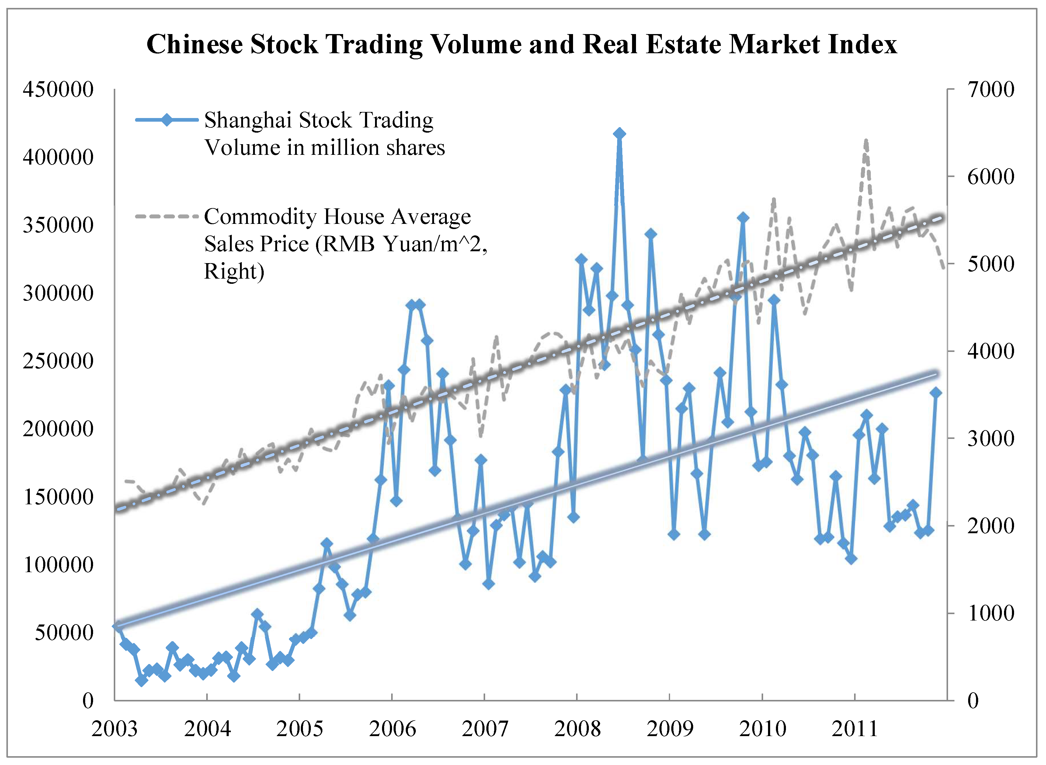
This paper explores the possible mechanisms by which housing affects household stock investment in China, a transitional economy that experienced both housing privatization reform and financial market construction in the past 30 years. Prior to the economic reforms, housing in urban China was provided to households based on their work units (employers). The housing privatization reform initiated in 1994 transformed the housing market in China from planned economy orientated into commercialized. The released housing demand from the urban population coupled with massive migration in the urbanization process in China resulted in excessive housing demand, relative to the limited housing supply. Additionally, because of the strong driving effects of the real estate industry on the steel, glass, cement, chemical, and many other industries, the Chinese government has been supporting the housing markets by means of monetary and fiscal stimuli. Consequently, the national average of housing prices has experienced one-way increases since the inception of house markets. In the period 2003–2009, overall the residential housing prices in 35 cities, as reported by the National Development and Reform Commission of China, approximately doubled. Parallel with the housing reform, the stock markets in China were established in 1991. Albeit full of bubbles and crashes, Chinese equity markets have been growing into one of the largest in capitalization around the world. The contemporaneous trending between the Chinese real estate market and the stock market is showed in Figure 1. It can be seen that the housing price index indicates a consistent increasing trend in the past decade. The stock market trading volume also shows an increasing trend although there are unpredictable ups and downs. The trend lines of the two series are shown in Figure 1 as well (monthly data, 2003–2011).

Studying how housing affects the homeowners’ stock investment in the context of China provides policy references for countries that undergo housing privatization reforms (where access to housing was disassociated from state employment and property rights were transferred from the state to individuals).

We investigate the mechanism by which housing affects household stock investment through a structure equation model (SEM). Previous studies usually applied conventional regression analysis, in which independent variables contain interlinked variables (e.g., house value, household wealth, and house-to-wealth ratio). The regression analysis offers a ceteris paribus causal relationship of housing variables on stock investment, but it cannot describe diverse paths by which housing-related variables simultaneously affect stock investments. SEM is advantageous in terms of dealing with relations involving multiple paths and interlinked variables. It is widely used in research on psychology, management, and marketing, but rarely on housing economics. An SEM approach enables us to examine the complex effects of housing on stock investment concurrently.

We reveal three channels through which housing significantly affects household stock investment. The first channel is through a “wealth effect”. When house value appreciates (depreciates), it sequentially increases (decreases) household wealth. The increased (decreased) wealth encourages (discourages) the households in stock investment. The second channel is through a “crowd-out effect”. When house value appreciates (depreciates), it simultaneously causes the house-to-wealth ratio to increase (decrease); the concentration of household wealth in housing brings greater background risk to the household. As a consequence, the household would reduce the equity investment so as to decrease the household’s overall risk level. The last channel is through a “direct effect” from housing to stock investment. The “direct effect” channel implies that there are other unobservable confounding variables that affect both housing and stock investment.

Applying the data from China Household Finance Survey (CHFS) in 2011, we confirm and quantify the contemporaneous “wealth effect” and “crowd-out effect” of housing on household equity investment. In addition, we also find a positive direct effect of housing on stock investment. Overall, house appreciation generates combined positive effect on stock investment among urban households in China. Given a house value appreciation of ¥10,000 on average, we find that predicted stock market participation probability increases 2.8% and that stock share in the household financial portfolio increases 12.8%.

The remainder of the paper is organized as follows. Section 2 introduces methods, sets up the structure equation model (SEM) and describes data and variables. Section 3 presents SEM results. Section 4 discusses results in the context of the housing market in China. Section 5 concludes.

2. Model, Data, and Variables

2.1. Structural Equation Model

In contrast to previous literature, we employed the SEM approach to explore the underlying mechanisms by which housing affects homeowners’ stock investments. SEM is a multivariate statistical analysis technique that is used to analyze structural relationships. This technique is the combination of factor analysis and multiple regression analysis, and it is used to analyze the structural relationship between measured variables and latent constructs. The SEM method was preferred by the researcher because it could estimate the multiple and interrelated dependences in a single analysis (Anderson and Gerbing 1988). Initiated by Wright (1934) and synthesized by Jöreskog (1970, 1973), the SEM method has been widely applied in many fields, such as psychology (MacCallum and Austin 2000), management (Shah and Goldstein 2006), and behavioral science (Spirtes et al. 1998). Nonetheless, few researchers have applied the SEM method in household finance studies.

Relative to the conventional regression approach, which only offers the ceteris paribus causal relationships between dependent and independent variables, the SEM approach is advantageous in terms of establishing complex causal relationship among variables, which enables it to conduct multiple path analysis and measure separate effects of interlinked variables on the response variable. By combining the respective effects from interlinked housing variables (e.g., house value, household wealth, and house-to-wealth ratio), the SEM approach is capable of finding the combined effects from interlinked housing variables on household equity investment.

Our SEM analysis focused on the analysis of the path through which housing-related variables simultaneously affect stock investment. As discussed in the previous section, many previous papers have reported either “wealth effect” or “crowding–out effect” of housing on stock investment. It is possible that there are other unknown channels through which housing affects stock investment besides “wealth effect” and “crowd-out effect”. To represent those unknown channels, we considered a direct effect, from house appreciation (depreciation) to stock investment directly. The effects of multiple housing-related variables on household stock investment and the cross relations among variables were represented through the equation system below1:

$$\begin{array}{cc}\hfill Stock\mathrm{In}v& ={\beta }_{1}HouseApp+{\beta }_{2}House2Wealth+{\beta }_{3}Wealth+{\Gamma }_{1}Controls+{\epsilon }_1\hfill \\ \hfill House2Wealth& ={\beta }_{4}HouseValue+{\beta }_{5}Wealth+{\epsilon }_2\hfill \\ \hfill Wealth& ={\beta }_{6}HouseValue+{\beta }_{7}StockInv+{\Gamma }_{2}Controls+{\epsilon }_3\hfill \\ \hfill HouseValue& ={\beta }_{8}HouseApp+{\Gamma }_{3}Controls+{\epsilon }_4\hfill \\ \hfill HouseApp& ={\Gamma }_{4}Controls+{\epsilon }_5\hfill \end{array}$$

(1)

The first equation shows that stock investment (StockInv) is dependent on house appreciation/depreciation (HouseApp), household wealth (Wealth), house to wealth ratio (House2Wealth), and control variables (Controls). Referring to the extant literature, our control variables included: Age, age squared, gender, education, marriage status, and risk attitude of the household head. At the household level, we also included family size, household aggregate loans, and the region where the household was located. The second equation indicates that the house-to-wealth ratio is determined by house value and household wealth. The third equation illustrates that household wealth depends on housing assets, stock investment, and control variables regarding the household. The fourth equation shows that current house value is related to house appreciation/depreciation and aforementioned control variables. The fifth equation presents the idea that house appreciation (depreciation) is independent of household wealth and household stock investment and influenced by control variables.

Corresponding to the above equation system, the path diagram reflecting the effects of housing on stock investment is shown in Figure 2. House appreciation/depreciation (HouseApp) was considered as an independent variable; wealth (Wealth) and house-to-wealth ratio (House2Wealth) were treated as mediator variables. Stock investment was the ultimate response variable measured by stock ownership (StockOwnership) and stock share (StockShare).

Two things are worthy of explanation in the diagram. One is that HouseApp affects stock investment, but not vice versa. This reflects the fact that house prices are mainly influenced by government policies other than households’ investment choices in China. Although the housing reform allows supply and demand to determine house prices, governments still have a full control on house supply and administrative measures to affect demand such as tax rates, mortgage loan rates, and a quota system determining how many house units a household can purchase at maximum. The governments’ policies and regulations on housing are beyond the control of any individual households. Rather, each household is affected by the abovementioned policies and regulations differently, based on the household demographic characteristics such as region, household head age, education, risk attitude, etc. Therefore, we filtered out these household’s characteristic variables in the diagram.

The other—is that Wealth is the summation of housing assets and non-housing assets net of all household debt. Therefore the value of the house (HouseValue) affects household Wealth through the coefficient of β₆ in the diagram; the value of stock investment (StockInv) affects household Wealth through the coefficient of β₇ in the diagram. The bidirectional relations between household Wealth and its StockInv are reflected in the coefficients of β₇ and β₃.

2.2. Data and Variables

The empirical estimation of SEM is based on the data from the China Household Finance Survey (CHFS), which is modeled on the Federal Reserve’s Survey of Consumer Finances in the US. The CHFS is conducted by the Southwestern University of Finance and Economics and covers 8438 households, consisting of 29,463 individuals in 80 counties in China, excluding Tibet, Xinjiang, Inner Mongolia, Hong Kong, and Macau. The survey uses method of three stages probability proportionate to size sampling (PPS) to ensure covering enough developed areas (coastal zones), urban households, and rich families. The CHFS survey is the first nationally representative household finance survey in China (Gan et al. 2013). Since China’s housing systems in rural and urban areas are quite different, we focused our analysis on urban households with a valid sample size of 3887.

We extracted three groups of variables from the CHFS data. The first group gives the details of household equity investments. Equity investment is the sum of direct stock investment and stock-type mutual funds. The second group variables are related to housing measures, such as house appreciation, the aggregate house value, and calculated house-to-wealth ratio. The third group variables contain socioeconomic information about households and household heads, including age, gender, marital status, educational level and risk attitude of the household head, the family size, household wealth, and household income, household loans, and the region in which the household is located. The summary statistics regarding these variables are reported in

Table 1. Variable definition and summary statistics.

	Definition of Variables	Mean	St. Dev.
Stock investments
StockOwnership	Households invest in stocks = 1, otherwise = 0	0.181	0.385
StockShare	The percentage of stock and stock-type mutual fund investment over total financial assets (%)	9.596	24.064
Housing variables
HouseApp	House appreciation calculated from community unit price and CPI adjusted house purchasing value (¥1000)	464.161	841.378
HouseValue	The aggregate house value calculated from average unit price in the community and the living area owned by the household (¥1000)	566.424	853.198
House2Wealth	House value over total household wealth	0.754	0.337
Demographic and household variables
Age	Age of household head	49.824	14.671
Sex	Gender of household head (male = 1, female = 0)	0.348	0.476
EduYr	Schooling years of household head	11.293	3.846
Marry	Marriage status of household head (married = 1, otherwise = 0)	0.835	0.371
RiskAtd	Self-reported attitude towards risk, higher value implies greater risk aversion. 1 (5.617%); 2 (8.412%); 3 (26.161%); 4 (17.902%); 5 (40.472%).
Wealth	Household wealth (¥1000)	666.172	986.932
FamilySize	Numbers of household members	3.053	1.258
HHInc	Household income (¥1000)	61.921	168.932
HHLoan	Household loan amounts (¥1000)	1.805	29.471
Region	East region = 1 (54.912%); Midlands = 2 (23.596%); West region = 3 (21.082%)

Notes: The statistics are calculated based on 3887 urban household observations from the China Household Finance Survey (CHFS) data in 2011. CPI—consumer price indexes.

.

Stock investment was firstly measured with StockOwnership, which represents the household’s stock market participation. It was equal to one if the household was involved in investment in either stock or stock-type mutual funds, zero otherwise. Another stock investment variable, StockShare, measures the degree of stock market participation. It was calculated as the percentage of stock investments over total financial assets. In our sample, there were 18.1% urban households having stock-type assets in their portfolio. The average of stock share was 9.60%.

HouseApp is the difference between current house value and house purchasing price adjusted by consumer price indexes (CPI). It is worth mentioning that, to avoid the possible measurement error from self-reported house value, the current household value was calculated from community unit house prices (excluding the studied household) where the household was located, multiplied by housing area of the household (we also re-estimated the SEM with self-reported house value, the results were similar). Relative to the current house value of ¥566.424, the average house appreciation was ¥464,161 per household, implying that, on average, about 82% of current house value resulted from house appreciation in our sample.

House2Wealth is the house-to-wealth ratio, measured by current total house value over household net wealth. The average of House2Wealth was 0.754. Predictably, the house was a dominant component of wealth for urban households.

3. Results

The estimation results from SEM are reported in

Table 2. Structural parameter estimates and goodness-of-fit indices.

	StockOwnership		StockShare
Coefficients	Estimate	t-Value	Estimate	t-Value
${\beta }_1$	−0.009	0.46	0.019 ***	2.50
${\beta }_2$	−0.046 ***	2.63	−0.045 ***	2.61
${\beta }_3$	0.063 ***	2.88	0.213 ***	7.28
${\beta }_4$	1.048 ***	21.29	1.033 ***	20.84
${\beta }_5$	−0.773 ***	15.70	−0.756 ***	15.25
${\beta }_6$	0.952 ***	192.1	0.946 ***	190.9
${\beta }_7$	0.002	0.36	0.042 ***	7.44
${\beta }_8$	0.583 ***	44.15	0.583 ***	44.15
${\Gamma }_1, {\Gamma }_2, {\Gamma }_3, {\Gamma }_4$	Omitted		Omitted
The goodness of fit indices	GFI = 0.9939, CFI = 0.9950, ECVI = 0.0225, RMSEA = 0.0867, NFI = 0.9948		GFI = 0.9943 CFI = 0.9954, ECVI = 0.0214, RMSEA = 0.0837, NFI = 0.9952

Note. We do not report the control variables’ coefficients for saving space (“omitted”). *** Coefficients are significant at the 0.01 level; ** Coefficients are significant at the 0.05 level; * Coefficients are significant at the 0.1 level.

. The goodness of fit statistics at the bottom of Table 2 show that the model structure is a good fit. All GFI, NFI, CFI indices were in the neighborhood of 0.99; ECVI was less than 0.05; and RMSEA was less than 0.10.

Corresponding to the estimated structure equations, the underlying paths that highlight the effects of housing on stock investment (StockOwnership and StockShare) are depicted in Figure 3 (StockOwnership) and Figure 4 (StockShare), respectively.

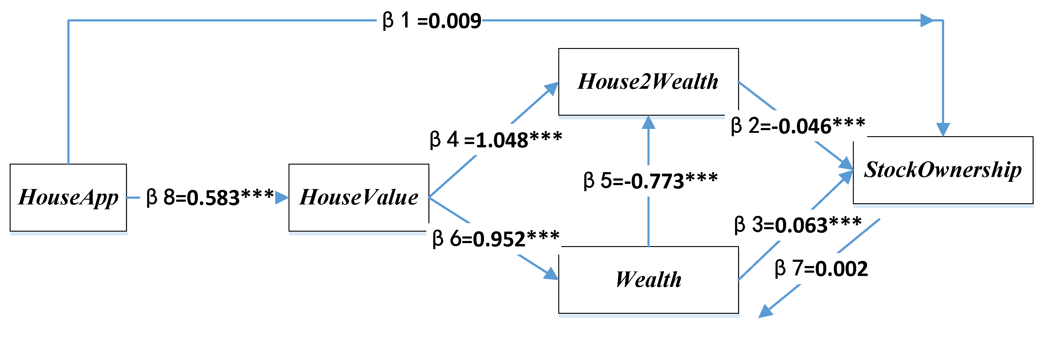
StockOwnership is a dummy variable. We transferred it into the predicted probability of a household participating in stock market before SEM estimation by applying the logistic regression method using control variables. When the stock investment was measured with stock ownership (StockOwnership), Figure 3 indicates all but two paths are significant. The path of the direct effect of house appreciation on stock ownership (β₁) and the path representing the effects of stock ownership on wealth (β₇) are statistically insignificant.

Based on the estimated path coefficients, we calculated the impact of housing-related variables on household stock ownership along diverse paths. It is clear to see that HouseApp positively affects HouseValue (β₈ = 0.583). The increased house value impacts household stock ownership through two mediator variables, wealth (Wealth) and house-to-wealth ratio (House2Wealth). Through the channel of “wealth”, the increased house value (HouseValue) significantly increased the household wealth (β₆ = 0.952). The “wealth effect” encouraged the households to participate in the stock market (β₃ = 0.063). When “House2Wealth” was treated as a mediator variable, HouseValue affected House2Wealth through two ways. One was that increased HouseValue directly extended House2Wealth (β₄ = 1.048) within the household. Another was that the changed wealth level resulting from HouseValue (β₅ = 0.952) reduced the value of House2Wealth (β₅ = −0.773). As a result, the combined effects of HouseValue on House2Wealth is 0.312 (=β₄ + β₆ × β₅ = 1.048 + 0.952 × (−0.773)). Consequently, House2Wealth negatively affected stock ownership through “crowd-out effects” (β₂ = −0.046). Overall, the comprehensive effect of housing on stock ownership was 0.028 (= ${\beta }_8\times \left({\beta }_6\times {\beta }_3+0.312\times {\beta }_2\right)$ = 0.583 × (0.952 × 0.063 − 0.312 × 0.046)). The combined positive coefficient implies that the predicted probability of stock market participation increased 2.8% when a household’s house appreciation increased by ¥10,000.

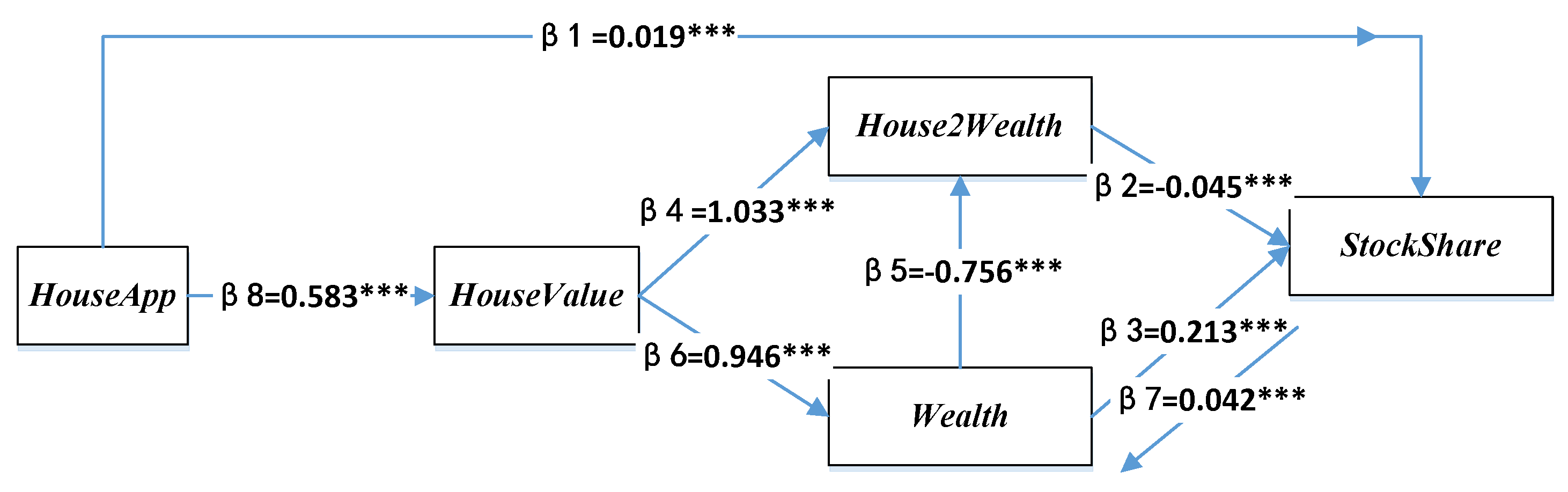
When household stock investment was measured with shares of stock in household financial portfolio (StockShare), we found three significant channels by which housing affected household stock investment simultaneously. First of all, HouseApp directly affected StockShare in a positive significant way (β₁ = 0.019). Similarly, the increased HouseValue resulting from house appreciation (HouseApp) impacted the StockShare through two mediator variables of Wealth and House2Wealth. Through the chain of Wealth (β₆ = 0.946), the “wealth effect” of housing on StockShare was positive (β₃ = 0.213). Through the chain of House2Wealth (0.318 = ${\beta }_4+{\beta }_6\times {\beta }_5$ = 1.033 + 0.946 × (−0.756)), the “crowd-out effect” from House2Wealth indicated a significant negative sign (β₂ = −0.045). Finally, the combined effect of housing on StockShare was 0.128 (=${\beta }_1+{\beta }_8\times \left({\beta }_6\times {\beta }_3+0.318\times {\beta }_2\right)$ = 0.019 + 0.583 × (0.946 × 0.213 − 0.318 × 0.045)). This coefficient implies that the shares of stock in household financial portfolio increased 12.8% if the house values appreciated by ¥10,000 in the household.

4. Discussions

Unlike extant literature which reports a single effect (either positive or negative) of housing on stock investment with the households, our analysis discloses the contemporaneous positive and negative effects of housing on stock investment and reconciles the controversial findings among the previous studies. Our findings of simultaneous positive and negative effects contribute to the current literature by providing new evidence of the relationships between housing and household financial asset allocation. Housing, as the dominant asset within the household, could affect household financing asset allocation through multiple ways. Emphasizing one key variable in the conventional regression analysis may ignore other underlying mechanisms by which housing affects equity investment. The application of SEM helps to figure out more reasonable channels that explain the effects of housing on stock investment. Examining the complicated relationships between housing and household stock investment in the context of China (a transitional economy that experienced both house privatization reform and the stock market construction in the past 20 years), could provide policy references for other transitional economies. In the process of transiting from planned economy to market economy, untying housing access from state jobs and releasing property right to private households may result in large house value appreciation, which as a consequence, generates the “wealth effect” and induces stock investment in the capital market. The booming property market could, to a certain degree, promote the prosperity of the capital market. However, this effect could be offset though the “crowd-out effect” as the house-to-wealth ratio increases. It is necessary to realize that homeowners are also rational investors; when the concentration of housing asset becomes larger within the household, the household could intentionally reduce its equity shares in the stock market. Therefore, a booming real estate market does not necessarily accelerate the development of the capital market.

In our SEM results analyses, the wealth effect of housing was represented by the coefficient of β₃, which is positive for both StockOwnership and StockShare. However we shall interpret the actual wealth effect to be greater than β₃. The reason is that our sample data covers a period of house price increase only. Kahneman and Tversky (1979) point out that the human brain treats losses (or potential losses) as more important than gains (or potential gains). Therefore, for a period of house price decrease, we would expect to see a much greater wealth effect.

In addition, we detected a direct effect from house appreciation on the shares of stock in the household financial asset. This effect is caused by something that is not considered by “wealth effect” and “crowd-out effect”. Due to the limited information of our survey data, we are unable to illustrate the detailed mechanism of this direct effect. It is possible that macroeconomic variables can address this positive “direct effect”. For example, interest rate dropping may bring prosperity to both the real estate market and stock market so that we observe a positive relation between house appreciation and stock value increase. In addition, investment behaviors could also be one of the reasons. Shiller (2005) indicates that “irrational exuberance” exists in housing bubbles and stock market booms.2 Further research could explore the possible channels behind the direct effect of housing on stock investment.

5. Conclusions

The extant literature regarding the effects of housing on household stock investment shows either positive or negative effects. This paper adopts an SEM approach to conduct a path analysis about how housing affects stock investments within the households. Applying the CHFS data in urban China, we find that the housing generates positive effect on households’ stock investment through a “wealth effect”. Concurrently, house-to-wealth ratio imposes a negative effect on household stock investment through a “crowd-out effect”. In addition, there are also other unknown channels through which housing affects stock investment. The combined effect of house appreciation on stock investment is positive.

Our findings open the black box of the effects of housing on stock investments. Not only do we reveal the coexistence of positive and negative effects of housing on stock investment, we also calculate the combined effects of housing on stock market participation and stock shares, respectively. In the context of urban China where housing prices have indicated a one-way increasing trend, the predicted probability of stock market participation increases 2.8% and the stock share in the household financial portfolio increases 12.8%, given the house value of homeowners appreciates by ¥10,000.

Our study provides policy references for the housing market and capital market in transition economies. At the same time, the conclusions drawn from this study are also meaningful for mature housing and investment markets, such as the US or European countries. On the one hand, the SEM analysis framework can be used to explore those market mechanisms. On the other hand, the combined positive effect of house appreciation on stock investment can be re-examined in those countries. Since the rapid housing price appreciation leads to an increased participation in the stock market, does this help to explain that a slump in real estate prices will cause stock investors to exit the stock market, as shown in the 2008–2012 global financial crisis? Future research could apply the SEM approach to investigate such issues and reveal multiple potential paths.

References

- Anderson, James C., and David W. Gerbing. 1988. Structural equation modeling in practice: A review and recommended two-step approach. Psychological Bulletin 1033: 411–23. [Google Scholar] [CrossRef]
- Briggs, Joseph S., David Cesarini, Erik Lindqvist, and Robert Östling. 2015. Windfall Gains and Stock Market Participation. Cambridge: National Bureau of Economic Research. [Google Scholar]
- Campbell, John Y., and Joao F. Cocco. 2003. Household risk management and optimal mortgage choice. The Quarterly Journal of Economics 118: 1449–94. [Google Scholar] [CrossRef]
- Campbell, John Y., and Joao F. Cocco. 2007. How do house prices affect consumption? Evidence from micro data. Journal of Monetary Economics 54: 591–621. [Google Scholar] [CrossRef]
- Cardak, Buly A., and Roger Wilkins. 2009. The determinants of household risky asset holdings: Australian evidence on background risk and other factors. Journal of Banking & Finance 33: 850–60. [Google Scholar]
- Chetty, Raj, and Adam Szeidl. 2015. The Effect of Housing on Portfolio Choice. Cambridge: National Bureau of Economic Research. [Google Scholar]
- Cocco, Joao F. 2004. Portfolio choice in the presence of housing. Review of Financial Studies 18: 535–67. [Google Scholar] [CrossRef]
- Flavin, Marjorie, and Takashi Yamashita. 2002. Owner-occupied housing and the composition of the household portfolio. The American Economic Review 92: 345–62. [Google Scholar] [CrossRef]
- Fougère, Denis, and Poulhes Mathilde. 2012. The Effect of Housing on Portfolio Choice: A Reappraisal Using French Data. Centre for Economic Policy Research (CEPR) Discussion Paper No. DP9213. Available online: http://ssrn.com/abstract=2210182 (accessed on 15 February 2013).
- Fratantoni, Michael C. 2001. Homeownership, committed expenditure risk, and the stockholding puzzle. Oxford Economic Papers 53: 241–59. [Google Scholar] [CrossRef]
- Li, Gan, Lu Zheng, Zhichao Yin, Nan Jia, and Shu Xu. 2013. Data You Need to Know about China: Research Report of China Household Finance Survey 2012. Berlin: Springer. [Google Scholar]
- Grossman, Sanford J., and Guy Laroque. 1990. Asset Pricing and Optimal Portfolio Choice in the Presence of Illiquid durable consumption goods. Econometrica 58: 25–51. [Google Scholar] [CrossRef]
- Jöreskog, Karl G. 1970. A general method for analysis of covariance structures with applications part ii: Applications. Biometrika 252: 239–51. [Google Scholar] [CrossRef]
- Jöreskog, Karl G. 1973. A General Method for Estimating a Linear Structural Equation System. In Structural Equation Models in the Social Sciences. New York: Seminar, pp. 85–112. [Google Scholar]
- Kahneman, Daniel, and Amos Tversky. 1979. Prospect theory: An analysis of decision under risk. Econometrica 472: 263–91. [Google Scholar] [CrossRef]
- MacCallum, Robert C., and James T. Austin. 2000. Applications of structural equation modeling in psychological research. Annual Review of Psychology 51: 201–26. [Google Scholar] [CrossRef] [PubMed]
- Meyer, Richard, and Kenneth Wieand. 1996. Risk and return to housing, tenure choice and the value of housing in an asset pricing context. Real Estate Economics 24: 113–31. [Google Scholar] [CrossRef]
- Michielsen, Thomas, Remco Mocking, and Sander Veldhuizen. 2016. Home Ownership and Household Portfolio Choice. New York: Social Science Electronic Publishing. [Google Scholar]
- Saarimaa, Tuuka. 2008. Owner-occupied housing and demand for risky financial assets: Some Finnish evidence. Finnish Economic Papers 21: 22–38. [Google Scholar]
- Shah, Rachna, and Susan Meyer Goldstein. 2006. Use of structural equation modeling in operations management research: Looking back and forward. Journal of Operations Management 24: 148–69. [Google Scholar] [CrossRef]
- Shiller, Robert. 2005. Irrational Exuberance: (Second Edition). Princeton and Oxford: Princeton University Press. [Google Scholar]
- Spirtes, Peter, Thomas Richardson, Christopher Meek, Richard Scheines, Richard Scheines, and Clark Glymour. 1998. Using path diagrams as a structural equation modeling tool. Sociological Methods & Research 272: 182–25. [Google Scholar]
- Turner, Tracy M., and Heather Luea. 2009. Homeownership, wealth accumulation and income status. Journal of Housing Economics 18: 104–14. [Google Scholar] [CrossRef]
- Wachter, Jessica A., and Motohiro Yogo. 2010. Why do household portfolio shares rise in wealth? Review of Financial Studies 23: 3929–65. [Google Scholar] [CrossRef]
- Wright, Sewall. 1934. The method of path coefficients. Annals of Mathematical Statistics 53: 161–215. [Google Scholar] [CrossRef]
- Yamashita, Takashi. 2003. Owner-occupied housing and investment in stocks: An empirical test. Journal of Urban Economics 53: 220–37. [Google Scholar] [CrossRef]