
Financial Deepening and Economic Growth Nexus in Nigeria: Supply-Leading or Demand-Following?


Abstract
:1. Introduction
2. Literature Review
2.1. Theoretical Framework
2.2. Empirical Literature
2.3. Limitations of Previous Studies
3. Methodology
3.1. Data and Sources
3.2. Model Specification
3.3. Description of Variables
3.4. Estimation Technique
4. Results and Discussion
5. Conclusions and Recommendations
5.1. Conclusions
5.2. Recommendations
Author Contributions
Conflicts of Interest
Appendix A
| VAR Granger Causality/Block Exogeneity Wald Tests | |||
| Date: 14 October 2015; Time: 13:32 Sample: 1970–2013 Included observations: 42 | |||
| Dependent variable: BA | |||
| Excluded | Chi-square | Degree of freedom | Probability |
| CR | 0.414173 | 2 | 0.8129 |
| GR | 0.365922 | 2 | 0.8328 |
| LR | 0.236432 | 2 | 0.8885 |
| MR | 0.578120 | 2 | 0.7490 |
| TR | 2.820104 | 2 | 0.2441 |
| All | 5.154918 | 10 | 0.8806 |
| Dependent variable: CR | |||
| Excluded | Chi-square | Degree of freedom | Probability |
| BA | 0.798868 | 2 | 0.6707 |
| GR | 2.270515 | 2 | 0.3213 |
| LR | 4.072561 | 2 | 0.1305 |
| MR | 3.126561 | 2 | 0.2094 |
| TR | 8.506981 | 2 | 0.0142 |
| All | 17.05607 | 10 | 0.0731 |
| Dependent variable: GR | |||
| Excluded | Chi-square | Degree of freedom | Probability |
| BA | 2.091518 | 2 | 0.3514 |
| CR | 2.467952 | 2 | 0.2911 |
| LR | 8.359085 | 2 | 0.0153 |
| MR | 3.733386 | 2 | 0.1546 |
| TR | 11.78489 | 2 | 0.0028 |
| All | 19.19907 | 10 | 0.0378 |
| Dependent variable: LR | |||
| Excluded | Chi-square | Degree of freedom | Probability |
| BA | 2.642556 | 2 | 0.2668 |
| CR | 0.759500 | 2 | 0.6840 |
| GR | 1.256911 | 2 | 0.5334 |
| MR | 0.255097 | 2 | 0.8803 |
| TR | 2.917831 | 2 | 0.2325 |
| All | 11.03855 | 10 | 0.3545 |
| Dependent variable: MR | |||
| Excluded | Chi-square | Degree of freedom | Probability |
| BA | 0.594002 | 2 | 0.7430 |
| CR | 0.123098 | 2 | 0.9403 |
| GR | 0.373803 | 2 | 0.8295 |
| LR | 9.406109 | 2 | 0.0091 |
| TR | 4.127024 | 2 | 0.1270 |
| All | 14.74395 | 10 | 0.1417 |
| Dependent variable: TR | |||
| Excluded | Chi-square | Degree of freedom | Probability |
| BA | 3.140361 | 2 | 0.2080 |
| CR | 5.028108 | 2 | 0.0809 |
| GR | 4.495025 | 2 | 0.1057 |
| LR | 3.062545 | 2 | 0.2163 |
| MR | 3.382383 | 2 | 0.1843 |
| All | 11.18014 | 10 | 0.3437 |
References
- Central Bank of Nigeria (CBN). Annual Report and Statement of Account. Abuja, Nigeria: Central Bank of Nigeria, 2003. [Google Scholar]
- World DataBank. “Explore. Create. Share: Development Data.” Available online: http://databank.worldbank.org/data/home.aspx (accessed on 24 July 2015).
- C.C. Soludo. The Global Financial Meltdown: Briefing of the Senate. Federal Capital Territory, Abuja: The Senate Chambers, 2008, pp. 1–15. [Google Scholar]
- International Monetary Fund (2014). “IMF Financial Access Survey.” Available online: http://fas.imf.org (accessed on 18 April 2016).
- A.E. Akinlo, and O. Akinlo. “Financial development, money, public expenditure and national income in Nigeria.” J. Soc. Econ. Dev. 1 (2007): 21–30. [Google Scholar]
- C.C. Agu, and J.O. Chukwu. “Multivariate causality between financial depth and economic growth in Nigeria.” Afr. Rev. Money Financ. Bank. 7 (2008): 7–21. [Google Scholar]
- O.J. Adelakun. “Financial sector development and economic growth in Nigeria.” Int. J. Econ. Dev. Res. Investig. 1 (2010): 25–41. [Google Scholar]
- S.O. Odeniran, and E.A. Udeaja. “Financial sector development and economic growth: Empirical evidence from Nigeria.” Cent. Bank Niger. Econ. Financ. Rev. 48 (2010): 92–124. [Google Scholar]
- Central Bank of Nigeria (CBN). Annual Report and Statement of Account. Abuja, Nigeria: Central Bank of Nigeria, 2014. [Google Scholar]
- J.A. Schumpeter. The Theory of Economic Development. Cambridge, MA, USA: Harvard University Press, 1911. [Google Scholar]
- C. Calderon, and L. Liu. “The direction of causality between financial development and economic growth.” J. Dev. Econ. 72 (2003): 371–394. [Google Scholar] [CrossRef]
- J. Gurley, and E. Shaw. “Financial structure and economic development.” Econ. Dev. Cult. Chang. 15 (1967): 333–346. [Google Scholar] [CrossRef]
- R.G. King, and R. Levine. “Finance and growth: Schumpeter might be right.” Q. J. Econ. 108 (1993): 717–737. [Google Scholar] [CrossRef]
- R. McKinnon. Money and Capital in Economic Development. Washington, DC, USA: Brookings Institution, 1973. [Google Scholar]
- J. Robinson. “The Generalization of the General Theory.” In Rate of Interest and Other Essays. London, UK: Macmillan, 1952. [Google Scholar]
- R.W. Goldsmith. Financial Structure and Development. New Haven, CT, USA: Yale University Press, 1969. [Google Scholar]
- W.S. Jung. “Financial development and economic growth: International evidence.” Econ. Dev. Cult. Chang. 34 (1986): 333–346. [Google Scholar] [CrossRef]
- M. Kar, and E.J. Pentecost. Financial Development and Economic Growth in Turkey: Further Evidence on the Causality Issue. Economic Research Paper No. 00/27; Loughborough, UK: Loughborough University, 2000. [Google Scholar]
- R.E. Lucas. “On the mechanics of economics development.” J. Monet. Econ. 22 (1988): 3–42. [Google Scholar] [CrossRef]
- G. Ndlovu. “Financial sector development and economic growth: Evidence from Zimbabwe.” Int. J. Econ. Financ. Issues 3 (2013): 435–446. [Google Scholar]
- D. Omotor. “Financial development and economic growth: Empirical evidence from Nigeria.” Niger. J. Econ. Soc. Stud. 49 (2007): 209–234. [Google Scholar]
- H. Apergis, and R. Levine. “Financial development and economic growth: A panel data analysis of emerging countries.” Int. Res. J. Financ. Econ. 8 (2007): 225–238. [Google Scholar]
- H.T. Patrick. “Financial development and economic growth in underdeveloped countries.” Econ. Dev. Cult. Chang. 14 (1966): 174–189. [Google Scholar] [CrossRef]
- T.M. Ibrahim, and M.I. Shuaibu. “Financial development: A fillip or impediment to Nigeria’s economic growth.” Int. J. Econ. Financ. Issues 3 (2013): 305–318. [Google Scholar]
- G.K. Sanni. “Foreign capital inflows, financial deepening and economic growth in Nigeria.” Niger. J. Econ. Soc. Stud. 54 (2012): 111–135. [Google Scholar]
- S.M. Nzotta. Money, Banking and Finance: Theory and Practice. Owerri, Nigeria: Hudson Jude Publishers, 2004. [Google Scholar]
- J.E. Ndebbio. Financial Deepening, Economic Growth and Development: Evidence from Selected Sub-Saharan African Countries. Nairobi, Kenya: African Economic Research Consortium, 2004. [Google Scholar]
- A.T. Johannes, A.M. Njong, and N. Cletus. “Financial development and economic growth in Cameroon, 1970–2005.” J. Econ. Int. Financ. 3 (2011): 367–375. [Google Scholar]
- M.A. Khan. “Financial development and economic growth in Pakistan evidence based on Autoregressive Distributed Lag (ARDL) Approach.” South Asia Econ. J. 9 (2008): 375–391. [Google Scholar] [CrossRef]
- S. Sahoo. “Financial Intermediation and Growth: Bank-Based versus Market-Based Systems.” Margin J. Appl. Econ. Res. 8 (2014): 93–114. [Google Scholar] [CrossRef]
- N.P. Audu, and T.P. Okumoko. “Financial development and economic growth in Nigeria.” Eur. J. Bus. Manag. 5 (2013): 69–81. [Google Scholar]
- C.C. Osuji, and E.E. Chigbu. “An evaluation of financial development and economic growth of Nigeria: A causality test.” Kuwait Chapter Arab. J. Bus. Manag. Rev. 1 (2012): 27–44. [Google Scholar]
- M.S. Nzotta, and J.E. Okereke. “Financial deepening and economic development of Nigeria: An empirical investigation.” Afr. J. Account. Econ. Financ. Bank. Res. 5 (2009): 52–66. [Google Scholar]
- E. Nkoro, and A.K. Uko. “Financial sector development-economic growth nexus: Empirical evidence from Nigeria.” Am. Int. J. Contemp. Res. 3 (2013): 87–94. [Google Scholar]
- S.O. Olofin, and U.J. Afangideh. “Financial structure and economic growth in Nigeria: A macro econometric approach.” Niger. J. Secur. Financ. 13 (2009): 1–27. [Google Scholar]
- J.A. Adams. “Financial intermediation and economic growth: Evidence from Nigeria.” J. Econ. Manag. 5 (1998): 27–40. [Google Scholar]
- M. Azege. The Impact of Financial Intermediation on Economic Growth: The Nigerian Perspective. Research Conference Paper for the Lagos State University; Lagos, Nigeria: Lagos State University, 2004. [Google Scholar]
- S. Johansen. “Statistical analysis of cointegrating vectors.” J. Econ. Dyn. Control 12 (1988): 231–254. [Google Scholar] [CrossRef]
- S. Johansen, and K. Juselius. “Maximum likelihood estimation and inference on cointegration with applications to the demand for money.” Bull. Econ. Stat. 52 (1990): 169–210. [Google Scholar] [CrossRef]
- C. Waqabaca. Financial Development and Economic Growth in Fiji. Working Papers, No. 03; Suva, Fiji: Economics Department, Reserve Bank of Fiji, 2004. [Google Scholar]
- A. Michael. “Financial development and economic growth: Is Schumpeter right? ” Br. J. Econ. Manag. Trade 2 (2012): 265–278. [Google Scholar]
- S.E. Mohammed, and M. Sidiropoulos. “Finance-Growth Nexus in Sudan: Empirical Assessment Based on an Application of the ARDL Model.” In Third International Student Conference Proceeding “Empirical Models in Social Sciences” (p. 47). 2006. Available online: Economics.soc.uoc.gr/macro/11conf/docs/sufian%205+final.doc (accessed on 15 April 2016).
- M.H. Pesaran, and Y. Shin. “The Ragner Frisch Contennial Symposium.” In An Autoregressive Distributed Lag Modelling Approach to Cointegration Analysis: Econometrics and Economic Theory in 20th Century. Edited by S. Storm. Cambridge, NY, USA: Cambridge University Press, 1999, pp. 354–391. [Google Scholar]
- G.S. Frank, and M.N. Eric. “Financial sector deepening and economic growth in Ghana.” J. Econ. Sustain. Dev. 3 (2012): 433–448. [Google Scholar]
- J. Thornton. “Financial deepening and economic growth: Evidence from Asian economies.” Sav. Dev. 18 (1994): 41–51. [Google Scholar]
- H.Y. Toda, and T. Yamamoto. “Statistical inferences in vector autoregressions with possibly integrated processes.” J. Econ. 66 (1995): 225–250. [Google Scholar] [CrossRef]
- R. Levine, N. Loayza, and T. Beck. “Financial intermediation and growth: Causality and causes.” J. Monet. Econ. 46 (2000): 18–41. [Google Scholar] [CrossRef]
- R. Levine, and S. Zervos. “Stock market development and long-run growth.” World Bank Econ. Rev. 10 (1996): 323–339. [Google Scholar] [CrossRef]
- J. Clarke, and S.A. Mirza. “Comparison of some common methods of detecting Granger non-causality.” J. Stat. Comput. Simul. 76 (2006): 207–231. [Google Scholar] [CrossRef]
- P.C.B. Phillips, and H.Y. Toda. “Vector autoregression and causality: A theorectical overview and simulation study.” Econ. Rev. 13 (1994): 259–285. [Google Scholar]
- R.F. Engle, and W.J.C. Granger. “Co-integration and error correction: Representation, estimation, and testing.” Econometrica 55 (1987): 251–276. [Google Scholar] [CrossRef]
- A.N. Rambaldi, and H.E. Doran. Testing for Granger Non-Causality in Cointegrated Systems Made Easy. Working Paper in Econometrics and Applied Statistics No. 88; Biddeford, ME, USA: University of New England, 1996. [Google Scholar]
- G.M. Caporale, and N. Pittis. “Efficient estimation of cointegrating vectors and testing for causality in vector autoregressions.” J. Econ. Surv. 13 (1999): 3–35. [Google Scholar]
- R. Levine. “Financial development and economic growth: Views and agenda.” J. Econ. Lit. 35 (1997): 688–726. [Google Scholar]

| Statistic | CR | BA | GR | LR | MR | TR |
|---|---|---|---|---|---|---|
| Mean | 13.08425 | 35.42234 | 4.402923 | 14.95818 | 17.33415 | 5.585111 |
| Median | 12.70369 | 32.90723 | 4.649226 | 16.75500 | 10.96388 | 5.403249 |
| Maximum | 38.34855 | 70.67310 | 33.73578 | 29.80000 | 73.75343 | 17.55881 |
| Minimum | 3.862077 | 14.93431 | −13.12788 | 6.000000 | 5.122039 | 0.148551 |
| Std. Dev. | 6.563540 | 13.24457 | 8.080945 | 6.406191 | 14.16887 | 3.500716 |
| Skewness | 1.930973 | 0.653420 | 0.963436 | 0.142541 | 2.376585 | 0.881809 |
| Kurtosis | 8.141648 | 2.867451 | 6.407793 | 2.151042 | 9.170601 | 4.436761 |
| Jarque–Bera | 75.81047 | 3.163231 | 28.09746 | 1.470337 | 111.2264 | 9.486820 |
| Probability | 0.000000 | 0.205643 | 0.000001 | 0.479425 | 0.000000 | 0.008709 |
| Sum | 575.7068 | 1558.583 | 193.7286 | 658.1600 | 762.7026 | 245.7449 |
| Sum Sq. Dev. | 1852.442 | 7543.001 | 2807.972 | 1764.689 | 8632.543 | 526.9655 |
| Observations | 44 | 44 | 44 | 44 | 44 | 44 |
| CR | BA | GR | LR | MR | TR | |
|---|---|---|---|---|---|---|
| CR | 1.000000 | 0.790731 | −0.339515 | −0.435276 | 0.351332 | 0.438212 |
| BA | 0.790731 | 1.000000 | −0.296440 | −0.361842 | 0.346332 | 0.420567 |
| GR | −0.339515 | −0.296440 | 1.000000 | 0.095854 | −0.345424 | 0.013725 |
| LR | −0.435276 | −0.361842 | 0.095854 | 1.000000 | −0.143523 | −0.159583 |
| MR | 0.351332 | 0.346332 | −0.345424 | −0.143523 | 1.000000 | 0.001028 |
| TR | 0.438212 | 0.420567 | 0.013725 | −0.159583 | 0.001028 | 1.000000 |
| Variable | ADF—Statistics | Adj. PP—Statistics | ||||
|---|---|---|---|---|---|---|
| Level | 1st Difference | 1st Difference Probability | Level | 1st Difference | Difference Probability | |
| GR | −5.738307 ** | −8.695053 ** | 0.0000 | −5.746942 ** | −13.98251 ** | 0.0000 |
| BA | −3.112282 ** | −5.727581 ** | 0.0000 | −2.105332 | −5.762296 ** | 0.0000 |
| CR | −3.152003 ** | −5.877677 ** | 0.0000 | −2.504949 | −9.433591 ** | 0.0000 |
| MR | −4.613153 ** | −9.848226 ** | 0.0000 | −4.709791 ** | −19.43562 ** | 0.0001 |
| TR | −2.460042 | −8.538936 ** | 0.0000 | −2.289743 | −9.596494 ** | 0.0000 |
| LR | −1.581782 | −10.27717 ** | 0.0000 | −2.034354 | −10.36160 ** | 0.0000 |
| (a) Trace statistic co-integration result | |||
| Hypothesized No. of CE(s) | Eigenvalue | Trace Statistic | 5% Critical Value |
| None * | 0.641836 | 129.1621 | 94.15 |
| At most 1 * | 0.582497 | 87.06481 | 68.52 |
| At most 2 * | 0.477041 | 51.25285 | 47.21 |
| At most 3 | 0.304575 | 24.67448 | 29.68 |
| At most 4 | 0.174228 | 9.781959 | 15.41 |
| At most 5 | 0.046053 | 1.933035 | 3.76 |
| (b) Maximum eigenvalues co-integration result | |||
| Hypothesized No. of CE(s) | Eigenvalue | Max–Eigen Statistic | 5% Critical Value |
| None † | 0.641836 | 42.09731 | 39.37 |
| At most 1 † | 0.582497 | 35.81197 | 33.46 |
| At most 2 | 0.477041 | 26.57836 | 27.07 |
| At most 3 | 0.304575 | 14.89252 | 20.97 |
| At most 4 | 0.174228 | 7.848924 | 14.07 |
| At most 5 | 0.046053 | 1.933035 | 3.76 |
| Dependent Variable: GR | |||
|---|---|---|---|
| Excluded | Chi-square | Degree of freedom | Probability |
| BA | 2.091518 | 2 | 0.3514 |
| CR | 2.467952 | 2 | 0.2911 |
| LR | 8.359085 | 2 | 0.0153 |
| MR | 3.733386 | 2 | 0.1546 |
| TR | 11.78489 | 2 | 0.0028 |
| All | 19.19907 | 10 | 0.0378 |
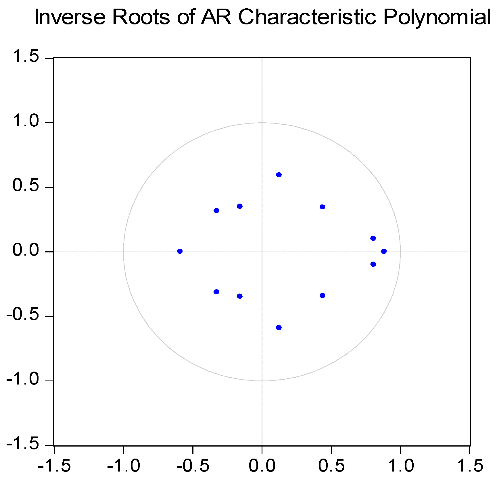
| Root | Modulus |
|---|---|
| 0.884875 | 0.884875 |
| 0.807974 − 0.099972i | 0.814135 |
| 0.807974 + 0.099972i | 0.814135 |
| 0.126250 − 0.591362i | 0.604688 |
| 0.126250 + 0.591362i | 0.604688 |
| −0.587398 | 0.587398 |
| 0.442022 − 0.342579i | 0.559235 |
| 0.442022 + 0.342579i | 0.559235 |
| −0.323339 − 0.315568i | 0.451808 |
| −0.323339 + 0.315568i | 0.451808 |
| −0.155795 − 0.348988i | 0.382184 |
| −0.155795 + 0.348988i | 0.382184 |
© 2017 by the authors. Licensee MDPI, Basel, Switzerland. This article is an open access article distributed under the terms and conditions of the Creative Commons Attribution (CC BY) license ( http://creativecommons.org/licenses/by/4.0/).
Share and Cite
Karimo, T.M.; Ogbonna, O.E. Financial Deepening and Economic Growth Nexus in Nigeria: Supply-Leading or Demand-Following? Economies 2017, 5, 4. https://doi.org/10.3390/economies5010004
Karimo TM, Ogbonna OE. Financial Deepening and Economic Growth Nexus in Nigeria: Supply-Leading or Demand-Following? Economies. 2017; 5(1):4. https://doi.org/10.3390/economies5010004
Chicago/Turabian StyleKarimo, Tari Moses, and Oliver Ejike Ogbonna. 2017. "Financial Deepening and Economic Growth Nexus in Nigeria: Supply-Leading or Demand-Following?" Economies 5, no. 1: 4. https://doi.org/10.3390/economies5010004