
The Determinants of Carbon Intensities of Different Sources of Carbon Emissions in Saudi Arabia: The Asymmetric Role of Natural Resource Rent

Department of Finance, College of Business Administration, Prince Sattam bin Abdulaziz University, 173, Alkharj 11942, Saudi Arabia
Economies 2023, 11(11), 276; https://doi.org/10.3390/economies11110276
Submission received: 8 October 2023
/
Revised: 26 October 2023
/
Accepted: 1 November 2023
/
Published: 7 November 2023
Abstract
:Natural resource rent (NRR) can be a blessing for the economic growth of resource-rich economies but may cause environmental problems. The present research explores the effects of NRR, economic growth, trade openness (TO), and foreign direct investment (FDI) on the carbon intensities of different sources of carbon emissions in Saudi Arabia from 1968 to 2021. The environmental Kuznets curve (EKC) is substantiated in the relationship between economic growth and the carbon intensities of gas emissions and cement emissions in the long run. The EKC is also validated in models of the carbon intensities of oil emissions, gas flaring emissions, and aggregated CO2 emissions in the short run. TO reduces the carbon intensities of oil emissions, gas emissions, and cement emissions in the long run. FDI mitigates the carbon intensity of gas flaring emissions but increases the carbon intensity of cement emissions. NRR increases the carbon intensities of all investigated sources of emissions in a linear analysis. In a nonlinear analysis, increasing NRR increases and decreasing NRR reduces the carbon intensities of all sources of emissions except aggregated CO2 emissions. In the short-run results, TO decreases the carbon intensity of gas flaring emissions and increases the carbon intensities of gas emissions and cement emissions. FDI decreases the carbon intensities of all sources of emissions. In a linear analysis, NRR reduces the carbon intensities of oil emissions and cement emissions and increases the carbon intensities of gas emissions and gas flaring emissions. In a nonlinear analysis, increasing NRR reduces the carbon intensity of cement emissions and increases the carbon intensities of gas emissions and gas flaring emissions. Moreover, decreasing NRR reduces the carbon intensities of gas emissions, gas flaring emissions, and aggregated CO2 emissions and increases the carbon intensities of oil emissions and cement emissions. The effect of NRR is asymmetrical in models of the carbon intensities of aggregated CO2 emissions, oil emissions, and gas flaring emissions and symmetrical in models of the carbon intensities of gas emissions and cement emissions.
1. Introduction
The Saudi economy is excessively dependent on the oil sector and stands in 2023 in the second position in the world with 297.5 billion barrels in oil reserves and more than 17% of global oil reserves (World Population Review 2023). Similarly, this economy holds the fifth position in terms of natural gas reserves and possesses more than 4% of global gas reserves (Worldometer 2023). In 2021, natural resource rent (NRR) from the gas and oil sectors accounted for 25% of income (World Bank 2023). On the consumption side, the Saudi economy ranks sixth in the world in fossil fuel consumption (Worldometer 2023). Both the production and consumption of fossil fuels are highly polluting, and the Saudi economy stood in the ninth position in the year 2021 in terms of CO2 emissions per capita (World Bank 2023). This intensive pollution is responsible for the Saudi Arabian economy’s high carbon intensity (CI), which is primarily due to its dependence on natural resources.
After this discussion of the environmental situation of Saudi Arabia, the role of international agencies in mitigating pollution emissions to reduce global warming is discussed. For instance, the Paris Agreement and the Sustainable Development Goals aim to decrease pollution emissions. To meet their target, one solution is very simple: reduce overall energy consumption, which could obstruct economic growth. However, no economy would agree to sacrifice economic growth to meet a target of reducing emissions. Thus, economies should focus on reducing their emissions per unit of Gross Domestic Product (GDP), which is termed carbon intensity (carbon emissions/GDP). Hence, economies should aim to reduce carbon intensity instead of reducing absolute emissions (Okorie and Wesseh 2023). In the case of the Saudi economy, one quarter of the country’s GDP depends on NRR, and NRR might affect the environment or the carbon intensity directly and indirectly. Directly, NRR stems from oil and gas production in Saudi Arabia, and pollution emissions both upstream and downstream of these sectors must be reduced. However, NRR might increase or decrease emissions indirectly. For instance, NRR supports the income of the country, which can be used for the development of renewable energy or energy-efficient technologies for non-resource sectors. Moreover, NRR can be used for the development of less-polluting sectors of the economy, with the intention of economic transformation. Thus, NRR can reduce carbon emissions and intensity through technique and composition effects. However, income from NRR can also increase emissions via a scale effect because of the increasing demand for energy-intensive products.
Trade openness (TO) may also determine carbon intensity. The balance of trade is a component of the GDP, and Saudi Arabia experienced a surplus in most of the sample period. Therefore, trade affects the GDP, the denominator of carbon intensity. Moreover, trade can also affect carbon emissions, the numerator of carbon intensity. For example, trade may increase economic activities and energy demand. Thus, trade can increase emissions through a scale effect (Grossman and Krueger 1991). Foreign direct investment (FDI) may serve the purpose of filling the gap between saving and investment in an economy and may also increase economic activities and energy demand. Moreover, FDI in Saudi Arabia mostly flows into the mineral sector (OECD 2020), which is pollution-oriented. Thus, FDI can increase both the GDP and carbon emissions. Conversely, FDI and TO may produce knowledge spillovers in the recipient country (Grossman and Helpman 1991), which may generate technique effects in the economy and reduce carbon emissions. In addition, TO and FDI may transform dirty industries into clean industries (Arrow et al. 1995; Vukina et al. 1999), which promotes the composition effect in an economy. Therefore, both the technique and composition effects of FDI and TO might mitigate carbon emissions and intensity (Letchumanan and Kodama 2000; Komen et al. 1997). Moreover, Grossman and Krueger (1991) suggested a nonlinear relationship between economic growth and emissions, which is known as the environmental Kuznets curve (EKC). In the EKC, economic growth initially harms the environment via a scale effect. However, environmental problems can be reduced at a later stage by achieving technique and composition effects.
The Saudi literature has probed the roles of income, energy variables, renewable energy consumption (REC), innovation, FDI, urbanization, and industrialization on carbon intensity (Aziz and Khan 2022; Kahia et al. 2023; Ali et al. 2023). Kahia et al. (2023) found an insignificant effect of FDI on aggregated CI in Saudi Arabia, and Ali et al. (2023) reported a negative effect of FDI on aggregated CI. Thus, the effect of FDI on aggregated CI is inconclusive in the Saudi literature. Moreover, the effect of NRR on CI has not been explored in the natural-resource-rich economy of Saudi Arabia. Furthermore, the effect of natural resources on aggregated carbon intensity has been examined in most of the global literature (Özkan et al. 2023; Thombs 2022; Abraham 2021). Therefore, the present study contributes to the literature by probing the effect of NRR on the CIs of different sources of emissions, i.e., natural gas flaring (NGF) emissions, oil emissions, natural gas emissions, and cement emissions. Thombs (2022) suggested performing an asymmetrical analysis of the relationship between CI and natural resources. Increasing NRR and decreasing NRR do not necessarily have the same signs and/or magnitudes in terms of their effect on CI. Thus, using nonlinear Autoregressive Distributive Lag (ARDL), the present research examines the asymmetrical effects of NRR on the aggregated and disaggregated CI variables in Saudi Arabia using the maximum range of available data from 1968 to 2021. Moreover, the literature has suggested investigating the nonlinear relationship between economic growth and CI to test the EKC (Lu et al. 2021; Li et al. 2019). Therefore, the present study hypothesizes a nonlinear relationship between economic growth and CI to investigate the EKC in Saudi Arabia.
2. Literature Review
The recent literature has changed its trend by investigating carbon intensity instead of carbon emissions. Several studies have examined the role of NRR in determining CI. For instance, Özkan et al. (2023) examined India from 1970 to 2020 and found that REC and natural resources helped to reduce carbon emissions and intensity. However, energy intensity and economic growth increased carbon emissions and intensity. Focusing on fossil fuels instead of aggregated natural resources, Thombs (2022) examined the asymmetrical effect of fossil fuels on CI in the United States (US) from 1999 to 2017 and found that increasing fossil fuels’ dependence on exports, consumption, and income increased carbon intensity. However, reducing fossil fuels’ dependence on exports and consumption did not affect carbon intensity. Nevertheless, the decreasing share of fossil fuels in income reduced CI. On the production side of fossil fuels, Abraham (2021) explored the US using state-level data and found that coal, oil, and gas production increased carbon intensity due to extractive emissions, lower energy efficiency, and subsidizing fuel. Similarly, Jing et al. (2020) claimed that oil refineries were a big source of increased carbon intensity.
Ren et al. (2020) suggested focusing on green finance to reduce fossil fuel dependency and CI. The authors examined China from 2000 to 2018 and found that green finance increased non-fossil fuel consumption and reduced CI. However, increasing the carbon intensity reduced green investment and non-fossil fuel consumption. Huang et al. (2023) introduced the role of green financial efficiency in combating CI in Chinese provinces from 2000 to 2019 and substantiated that green finance and green financial efficiency helped to reduce CI. In particular, green financial efficiency played a significant role in combating carbon intensity. Du (2023) introduced quantile regression analyses to the CI model and investigated 10 Asian economies. The author found that green finance and REC helped to reduce carbon intensity in all quartiles of regression. Yun (2023) contributed to the literature using monthly data from 2010 to 2020 in China and found that the GDP per capita increased natural resource consumption. Moreover, population density also increased natural resource consumption, which might increase carbon intensity.
The literature has also explored the effect of trade on carbon intensity. For example, Shi et al. (2022) examined China from 2000 to 2014 and found that the carbon intensity of exports increased from 2002 to 2014 and decreased after 2014. Industrial productivity helped to reduce carbon intensity, and energy intensity increased CI. In another country-specific study, Wang and Song (2022) explored the US and found that trade helped to reduce carbon intensity. Using provincial-level data, Chu et al. (2021) analyzed 30 Chinese provinces and corroborated that trade policy to reduce energy intensity helped to reduce carbon intensity. Moreover, the energy quota trading policy helped to reduce carbon intensity. Some studies analyzed a panel of economies instead of conducting a country-specific analysis. For instance, Wang et al. (2023b) examined the effect of trade on CI and substantiated that trade raised CI in 59% of investigated countries and reduced CI in the other 41% of countries. In particular, trade reduced CI in high-income countries and increased CI in low-income economies. Zhang et al. (2022) gave a new dimension to the carbon intensity literature by exploring the top ten emitters from 1990 to 2016 and found that REC reduced carbon intensity. However, exports, the stock market, and income inequality increased carbon intensity.
Zhong et al. (2022) augmented the role of environmental policies in a CI model of 43 economies from 2000 to 2014 and found that the export openness policy reduced the carbon intensity of exports. Moreover, the tight environmental policy also reduced CI. In a single-year analysis of 2014, Yang and Su (2019) analyzed 44 regions and found that exports increased carbon intensity at the global level. A country-level analysis also showed the same results. However, exports reduced carbon intensity in some sectors. Shao (2017) introduced the role of FDI to the relationship between trade and carbon intensity in 188 countries from 1990 to 2013 by developing panels of countries for different income groups. The results showed that FDI reduced carbon intensity in all investigated countries. Moreover, trade openness, fossil fuels, and industrial intensity also played their roles in this relationship. In a new dimension of research, Wang et al. (2023a) explored the effect of a single country’s FDI on the CI in 56 Belt and Road Initiative (BRI) economies from 2005 to 2018. The authors found that Chinese FDI in BRI countries helped to reduce carbon intensity in BRI economies. The levels of development, industrialization, and energy consumption in BRI economies also played their roles in this relationship.
Cheng and Yao (2021) added the impact of innovation to the CI model of 30 Chinese provinces from 2000 to 2015 and found that innovation in REC reduced carbon intensity. Xin and Wang (2022) proposed the role of institutional quality in the nexus between innovation and carbon intensity. The institutional quality in high-income countries helped to improve green scale effects, technical progress, and the composition of industries in BRI economies, which reduced carbon intensity. Zhang et al. (2023) introduced the role of environmental taxes to the relationship between innovation and CI in China and substantiated that environmental taxes increased environmental innovations. These innovations helped to reduce carbon emissions and intensity. Using a different approach, Okorie and Wesseh (2023) investigated the effect of the Paris Agreement on carbon intensity and found that this agreement helped to reduce carbon intensity and global emissions by 4.1%.
In a methodological development, Dai et al. (2022) explored China using a spatial analysis and found that local carbon emission trading helped to reduce carbon intensity in nearby areas. Moreover, technological progress played a mediating role in this spatial relationship. Guo and Tu (2023) introduced digital finance to a spatial CI model of 284 Chinese cities and substantiated that digital finance helped to reduce carbon intensity after a threshold point. Thus, the EKC was corroborated between these variables. Moreover, digital finance showed spillovers in neighboring cities as well. Ji et al. (2023) augmented digitalization in a spatial CI model of Chinese provinces from 2012 to 2019 and substantiated that digitalization reduced CI. Moreover, a decline in local CI had spillovers, which reduced CI in neighboring provinces.
In another methodological contribution, Wang and Wang (2021) introduced an asymmetrical analysis to examine the relationship among FDI, TO, and CI in 104 countries from 2000 to 2014 using a threshold model and substantiated that TO and FDI had an asymmetrical impact on carbon intensity. TO and FDI reduced CI in high-income nations and increased CI in upper-middle-income economies. In a larger sample of economies, Greiner and McGee (2020) analyzed the asymmetrical impact of economic progress on CI in 153 economies from 1960 to 2013 and found that falling economic activities reduced carbon intensity in developed nations. However, both rising and falling economic activities increased carbon intensity effectively in developing nations. In the relationship between economic growth and carbon intensity, Li et al. (2019) introduced the nonlinear effect of economic growth on CI to test the EKC in Chinese provinces and substantiated an inverted N-shaped relationship. Lu et al. (2021) advanced this idea by testing the EKC in the eight zones of China from 1997 to 2015 and found the N-shaped EKC between economic progress and CI in most of the investigated zones. Moreover, ecological policies and technologies mitigated carbon intensity. Mahmood et al. (2023a) advocated that the possibility of the existence of the EKC might increase if technology and REC reduced emissions in any economy.
A few studies have investigated the topic of carbon intensity in the Saudi literature. For instance, Aziz and Khan (2022) investigated Saudi Arabia from 1990 to 2019 and found that the GDP increased carbon intensity. However, REC and innovation reduced CI. Ali et al. (2023) contributed to the Saudi literature by testing the effect of urbanization on CI from 1991 to 2020 and substantiated that urbanization and energy consumption increased CI. However, FDI reduced carbon intensity. Kahia et al. (2023) tested the effect of REC on CI in Saudi Arabia from 1990 to 2018 and found that urbanization increased CI. However, FDI did not affect CI and REC mitigated CI. Moreover, the GDP, urbanization, and FDI raised CO2 emissions. However, innovation and REC reduced CO2 emissions. Sweidan (2018) investigated 13 MENA economies, including Saudi Arabia, from 1995 to 2013 and found that economic progress increased CI and that health spending reduced CI. Some studies on the MENA region investigated carbon emissions instead of carbon intensity. For instance, Belaïd and Massié (2023) examined Saudi Arabia from 1971 to 2020 and found that energy efficiency mitigated CO2 emissions. In a panel study, Mahmood et al. (2023b) investigated 17 MENA economies from 2000 to 2019 and validated the EKC. Moreover, oil rents increased CO2 emissions. However, FDI, innovation, and industrialization decreased CO2 emissions.
The literature has signified the importance of natural resources, trade, and FDI in determining carbon intensity. However, the role of NRR in determining CI is missing in the literature of the natural-resource-rich Saudi economy. Moreover, the literature suggested an asymmetrical analysis while investigating the factors of carbon intensity (Wang and Wang 2021; Greiner and McGee 2020). In particular, Thombs (2022) substantiated the asymmetrical effects of fossil fuel dependence on CI. Similarly, increasing and decreasing NRR could have different signs and/or magnitudes of effect on carbon intensity, which could be captured through an asymmetrical analysis. For instance, increasing NRR may increase the energy demand and CI if energy is sourced from fossil fuels. However, decreasing NRR may not decrease the energy demand and CI due to the ratchet effect or may not decrease the energy demand and CI with the same elasticity parameter as increasing NRR. Thus, the present research explores the asymmetrical impact of NRR on the CIs of oil emissions, natural gas emissions, NGF emissions, and cement emissions in Saudi Arabia from 1968 to 2021.
3. Methodology
Grossman and Krueger (1991) suggested a nonlinear relationship between economic growth and pollution emissions. Most of the carbon intensity literature has ignored this nonlinear relationship and has probed the linear impact of economic growth on carbon intensity (Aziz and Khan 2022; Yun 2023; Özkan et al. 2023). However, some recent studies suggested a nonlinear relationship between income and CI (Lu et al. 2021; Li et al. 2019). The present study also assumes a nonlinear relationship between economic growth and carbon intensity to scrutinize the EKC hypothesis. Moreover, FDI and trade may also affect carbon intensity through the channels of the GDP and carbon emissions. Both variables may increase the GDP by increasing the production level in an economy. Moreover, FDI and trade may accelerate carbon emissions via the scale effect of growth. Alternatively, both variables may also help to reduce carbon emissions via technique and composition effects. The technique effect might be achieved due to knowledge spillovers in the recipient country (Grossman and Helpman 1991). The composition effect would also be attained by shifting dirty industries into clean industries (Arrow et al. 1995; Vukina et al. 1999). Thus, FDI and trade may determine carbon intensity. NRR in a resource-rich country could have an impact on the GDP and emissions. NRR is a direct source of income and may enhance the GDP of the economy. Moreover, natural resource extraction may also pollute the environment. Thus, NRR can determine CI. In addition, NRR and CI could have endogeneity, as an economy with higher carbon intensity tends to improve its NRR. To address the endogeneity issue, the ARDL framework is utilized for estimation. ARDL solves the endogeneity problem via the autoregressive process and provides efficient results (Pesaran et al. 2001). The model of the study is as follows:
CIt is the carbon intensity variable, which is measured in aggregated (CO2Et) and disaggregated (OEt, GFEt, GEt, and CEt) forms. CO2Et is the natural logarithm of aggregate CO2 emissions per unit of GDP. In the same way, OEt, GFEt, GEt, and CEt are the natural logarithms of oil, natural gas flaring, natural gas, and cement emissions per unit of GDP, respectively. Thus, all proxies show the aggregated and disaggregated forms of carbon intensity. GDPCt is a proxy for economic growth and is the natural logarithm of GDP per capita. GDPCt2 is the square of GDPCt. TOt is the total trade percentage of GDP, and FDIt is the net FDI inflow percentage of GDP. NRRt is the total natural resource rent percentage of GDP. TOt, NRRt, and FDIt are not taken as logarithms, as these variables are percentages. Table 1 shows the data sources and expected signs of the coefficients of the variables.
To test the unit root, we use the MZa statistics of Ng and Perron (2001) with a null hypothesis of non-stationarity in the following way:
If the null hypothesis is rejected with the estimated MZa statistics, then the series is stationary. After confirming the unit root, we may find the long-run relationships and coefficients using the ARDL of Pesaran et al. (2001). The ARDL cointegration technique is efficient and provides robust results in the presence of a mixed order of integration. Furthermore, the ARDL technique also removes the effect of endogeneity in the model via the autoregressive process (Pesaran et al. 2001). The ARDL framework for Equation (1) is as follows:
Equation (3) is used to examine the cointegration via the bound test for each proxy of carbon intensity. Kripfganz and Schneider’s (2020) critical values are used for the bound test, which are efficient for small sample sizes. Later, long-run effects are captured by normalizing the coefficients (). Moreover, the short-run effects are estimated by replacing the lagged-level variables with the Error Correction Term (ECTt−1) in the following way:
A negative and significant can ensure the presence of the short-run relationships in Equation (4). Moreover, the short-run effects are captured by. This study supposes that NRRt could have an asymmetrical effect on carbon intensity. Therefore, the series NRRt is divided into two series according to Shin et al. (2014) in the following way:
Equation (5) develops NRRPt by taking the partial sum of the positive deviations in NRRt. Equation (6) develops NRRNt by taking the partial sum of the negative deviations in NRRt. Now, NRRPt and NRRNt are replaced with NRRt in Equation (3) to capture the long-run results from the nonlinear ARDL in the following way:
The Wald test is applied to the coefficients of NRRPt and NRRNt in Equation (7) to test the asymmetry in the relationship between NRR and carbon intensity. The lagged-level variables in Equation (7) are replaced with ECTt−1 for the short-run analysis in the following way:
All procedures of estimation for the ARDL in Equations (3) and (4) can be repeated for the nonlinear ARDL in Equations (7) and (8).
4. Data Analysis
Table 2 shows that the descriptive statistics and mean values of CO2Et, OEt, GDPCt, GDPCt2, TOt, and NRRt are greater than the Standard Deviations (SDs). Therefore, these variables are under-dispersed. However, the rest of the variables are over-dispersed. Moreover, the unit root test is applied to test the stationarity of all variables in Table 3.
Table 3 shows the unit root results. The estimated MZa statistics show that the null hypothesis of non-stationarity is rejected for TOt and NRRt at their levels with intercept specification at the 10% and 5% levels of significance, respectively. Thus, TOt and NRRt are stationary at their levels. Similarly, FDIt is also stationary at the 1% and 5% levels of significance with different specifications. However, the null hypothesis of non-stationarity cannot be rejected for the rest of the series, and the rest of the variables are non-stationary at their levels. The null hypothesis of non-stationarity is rejected for all variables at their first differences, and all variables are stationary. Thus, the integration level is mixed, as some independent variables are stationary at their levels. Therefore, the ARDL technique is applied, which provides robust results in the presence of a mixed order of integration.
Table 4 and Table 5 show the long and short results of the ARDL models after the selection of the optimal lag length using the Schwarz Information Criterion (SIC). The lag lengths are shown in the second column as per the models in the first column. The cointegration is not substantiated in the model of the carbon intensity of aggregate CO2 emissions. However, the cointegration is proven in this model by the negative and significant coefficient of ECTt−1, as shown in Table 6 (Pesaran et al. 2001). Moreover, the cointegration is substantiated in the models of the carbon intensities of oil emissions, gas emissions, gas flaring emissions, and cement emissions at the 10%, 1%, 5%, and 1% levels of significance, respectively. The validity of the cointegration is consistent in the case of both linear and nonlinear ARDL techniques. Therefore, the cointegration is substantiated in all linear and nonlinear ARDL models. In addition, diagnostic tests are performed to test heteroscedasticity using the Breusch–Pagan–Godfrey test (Breusch and Pagan 1979), serial correlation using the Breusch–Godfrey test (Breusch 1978; Godfrey 1978), the normality of the error term using the Jarque–Bera test (Jarque and Bera 1987), and functional form using the Ramsey RESET test (Ramsey 1969). The p-values of all diagnostic tests are greater than 0.1 and indicate that the models do not have any econometric problems.
The long-run results are estimated and presented in Table 5. The coefficients of GDPCt and GDPCt2 are positive and negative, respectively, in the linear and nonlinear models of the carbon intensities of gas emissions and cement emissions. Thus, the EKC is substantiated in the models of the carbon intensities of gas emissions and cement emissions. Increasing economic growth raises the carbon intensities of gas emissions and cement emissions initially and reduces the carbon intensities afterward. Similarly, Lu et al. (2021) and Li et al. (2019) also substantiated the EKC in China in symmetrical analyses. However, the present study hypothesizes a more dynamic model by incorporating the asymmetrical effect of NRR in the EKC model. Moreover, the literature did not investigate the EKC in the carbon intensity model of Saudi Arabia but reported a positive linear impact of economic growth on carbon intensity (Aziz and Khan 2022; Kahia et al. 2023). The EKC cannot be validated for the carbon intensities of oil emissions, gas flaring emissions, and aggregate CO2 emissions. The linear and nonlinear ARDL models reach the same conclusions, and each model confirms the robustness of the other model.
Trade openness has a negative effect on the CIs of oil emissions, gas emissions, and cement emissions. Thus, trade openness is found to be helpful in reducing the carbon intensities of oil emissions, gas emissions, and cement emissions. This effect can be explained from two sides. Firstly, trade openness may increase the GDP of Saudi Arabia as the balance of trade is surplus in most sample years. Secondly, trade openness encourages clean technologies in production and could reduce CO2 emissions. Similarly, the literature has substantiated the negative impact of trade on CI in high-income nations using an asymmetrical analysis (Wang and Wang 2021) and symmetrical analyses (Wang et al. 2023b; Wang and Song 2022). However, these studies did not analyze the disaggregated carbon intensities of different sectors and did not specifically analyze the oil-rich economy of Saudi Arabia. Thus, the present research exploits this opportunity and finds a negative impact of trade openness on the CIs of the oil, gas, and cement sectors in the oil-rich and high-income economy of Saudi Arabia. However, TOt has no effect on the carbon intensities of gas flaring emissions and aggregate CO2 emissions. The results of the linear ARDL are consistent with the nonlinear ARDL, which confirms the robustness of the results in all the aggregated and disaggregated CI models.
The results of the present study show that FDI has no impact on the aggregated CI in Saudi Arabia. Similarly, Kahia et al. (2023) found an insignificant effect of FDI on the aggregated carbon intensity in Saudi Arabia. However, Ali et al. (2023) found a negative effect of FDI on CI. Both studies used symmetrical analyses. However, by conducting an asymmetrical analysis and using disaggregated proxies of carbon intensity, the present study solves this inconclusive debate on the relationship between FDI and carbon intensity. For instance, FDI reduces the carbon intensity of gas flaring emissions in the present study. Thus, FDI helps to increase the GDP of Saudi Arabia and/or decrease emissions from gas flaring. In the non-Saudi literature and aggregated carbon intensity analyses, some studies also validated the negative influence of FDI on carbon intensity (Wang and Wang 2021; Shao 2017; Wang et al. 2023a). Alternatively, FDI raises the CI of cement emissions in the present research. This result is natural, as the cement sector is highly polluted and is responsible for a higher carbon intensity. Moreover, the cement sector is highly dependent on coal, which is the largest source of emissions. Wang and Wang (2021) also reported a positive effect of FDI on CI in upper-middle-income economies. The effect of FDI on CI is consistent in the results of both the linear and nonlinear ARDL models, which substantiates the robustness of the results.
In the results of the linear ARDL, NRR raises the carbon intensities of oil emissions, gas emissions, cement emissions, gas flaring emissions, and aggregate CO2 emissions. NRR always contributes to the GDP of the resource-rich economy of Saudi Arabia. However, this result shows that NRR has contributed to emissions to a greater extent than the GDP. Thus, NRR is an environmental concern for this economy. Similarly, Mahmood et al. (2023b) found that oil rents increased aggregated CO2 emissions in symmetrical analyses of the MENA region. In contrast, Özkan et al. (2023) found that NRR reduced carbon intensity in an aggregated and symmetrical analysis of India. However, in the asymmetrical and disaggregated analyses, the present study substantiates that increasing NRR raises the carbon intensities of oil emissions, gas emissions, gas flaring emissions, and cement emissions. Similarly, decreasing NRR has a positive effect on the CIs of oil emissions, gas emissions, gas flaring emissions, and cement emissions. Thus, increasing NRR increases the carbon intensities of oil emissions, gas emissions, gas flaring emissions, and cement emissions, and decreasing NRR decreases the carbon intensities of these sources of emissions. Nevertheless, the effect of NRR on the CIs of oil emissions, aggregated CO2 emissions, and gas flaring emissions is asymmetrical in terms of magnitude. However, the effect of NRR on the CIs of gas emissions and cement emissions is symmetrical. The signs of the effects of NRR on CI are the same for all disaggregated proxies of carbon intensity. Therefore, the results are consistent and substantiate the robustness of the estimates from the linear and nonlinear ARDL.
Table 6 shows the short-run results. The coefficients of ECTt−1 are negative in the models of the carbon intensities of all sources of emissions. Thus, the short-run relationships are substantiated in both the linear and nonlinear ARDL models. The coefficients of ECTt−1 in the nonlinear ARDL models are greater than those in the linear ARDL models. This may be because the linear models ignore the possibility of nonlinear relationships between the variables. However, the nonlinear models care about the possibility of nonlinear relationships between the variables. Thus, the nonlinear models estimate more dynamic and stable relationships (Anderl and Caporale 2022). The EKC is substantiated in a model of the carbon intensity of the aggregated CO2 emissions in both the linear and nonlinear ARDL estimations. The EKC is also validated in the linear ARDL model of the carbon intensity of oil emissions and the nonlinear ARDL model of the carbon intensity of oil emissions with a one-year lag in economic growth. However, a U-shaped association is found in the relationship between economic growth with a one-year lag and the CI of gas emissions in the linear and nonlinear models. The EKC is substantiated in the nonlinear ARDL model of the carbon intensity of gas flaring emissions and the linear ARDL model of the carbon intensity of gas flaring emissions with a one-year lag in economic growth. In the cement emissions model, the EKC is substantiated, and a U-shaped relationship is found with a one-year lag in economic growth.
In the short run, ΔTOt−1 has a positive effect on the carbon intensities of gas emissions and cement emissions. However, trade openness has a negative effect on the CI of gas flaring emissions. Moreover, FDI reduces the CIs of oil emissions, gas emissions, gas flaring emissions, and aggregated CO2 emissions. In addition, FDI with a one-year lag mitigates the carbon intensity of cement emissions. NRR raises the carbon intensities of gas emissions and gas flaring emissions. However, NRR mitigates the carbon intensity of cement emissions. Moreover, NRR with a one-year lag reduces the CI of oil emissions. In the asymmetrical analysis, increasing NRR raises the carbon intensities of gas and gas flaring emissions and mitigates the carbon intensity of cement emissions. Decreasing NRR mitigates the carbon intensities of gas flaring emissions and aggregated CO2 emissions. However, it has a negative effect on the carbon intensities of oil emissions and cement emissions. In addition, decreasing NRR with a one-year lag mitigates the carbon intensity of gas emissions. After the discussion of the long- and short-run results, Cumulative Sum (CUSUM) and CUSUM square (CUSUMsq) tests are performed to test the stability of the parameters from the ARDL and nonlinear ARDL models. The results are presented in Table 7. All graphs substantiate that the estimated CUSUM and CUSUMsq values are within the critical bound lines, which reflects the stability of the estimated parameters from the linear and nonlinear models.
The results of this study suggest that NRR increases the carbon intensities of most sources of emissions in the long-run estimates of the linear and nonlinear models. Therefore, NRR is a source of CO2 emissions that is increasing carbon intensity. A quarter of Saudi income and about 90% of exports and government spending are sourced from natural resource revenues. Therefore, Saudi Arabia should reduce its dependence on natural resources in terms of income, exports, and government spending to avoid the environmental problems stemming from NRR. The revenues from NRR can be utilized for the economic transition to shift the economy from the natural resource sector to some environmentally friendly sectors (Mahmood 2022). Furthermore, the Saudi economy should invest NRR in the development of renewable energy infrastructure, which would reduce CI. Moreover, TO and FDI help to reduce the CIs of most sources of emissions. Therefore, Saudi Arabia should liberalize the economy to enhance trade and attract more foreign investments. This effort can support a clean environment by reducing the CI in the investigated sectors and the entire economy. However, the results show that FDI raises CI in the cement sector. Thus, FDI in the cement sector should only be welcomed with clean energy technologies. Otherwise, the government should design tight environmental policies for this sector to ensure environmental sustainability.
5. Conclusions
NRR plays a role in determining income and emissions in the resource-rich economy of Saudi Arabia. Thus, the present research explores the asymmetrical effect of NRR on the CIs of different sources of CO2 emissions using data from 1968 to 2021. In the long run, the EKC is substantiated in the models of the carbon intensities of gas emissions and cement emissions. However, the EKC is not substantiated in the models of the carbon intensities of aggregated CO2 emissions, gas flaring emissions, and oil emissions. In the short run, the EKC is validated in the models of the carbon intensities of oil emissions, gas flaring emissions, and aggregated CO2 emissions. Nevertheless, a U-shaped association is substantiated in the models of the carbon intensities of gas emissions and cement emissions. Trade openness reduces the carbon intensities of oil emissions, gas emissions, and cement emissions in the long run. However, trade openness cannot affect the carbon intensities of aggregated CO2 emissions and gas flaring emissions. Moreover, FDI reduces the carbon intensity of gas flaring emissions but increases the carbon intensity of cement emissions. However, FDI has a statistically insignificant effect on the carbon intensities of aggregated CO2 emissions, oil emissions, and gas emissions. In the linear analysis, NRR increases the carbon intensities of all investigated sources of emissions. In the nonlinear analysis, increasing NRR increases CI, and decreasing NRR reduces the CIs of all sources of emissions except aggregated CO2 emissions. The effect of NRR is asymmetrical in the models of the carbon intensities of aggregated CO2 emissions, oil emissions, and gas flaring emissions. However, it is symmetrical in the models of the carbon intensities of gas emissions and cement emissions. In the short run, trade openness increases the carbon intensities of gas emissions and cement emissions. However, trade openness decreases the carbon intensity of gas flaring emissions. Nevertheless, trade openness has a statistically insignificant effect on the CIs of oil emissions and aggregated CO2 emissions. In addition, FDI decreases the carbon intensities of all sources of emissions. In the short-run linear analysis, NRR increases the carbon intensities of gas emissions and gas flaring emissions. However, NRR reduces the carbon intensities of oil emissions and cement emissions. Nevertheless, NRR cannot determine the carbon intensities of aggregated CO2 emissions and cement emissions. In the short-run nonlinear analysis, increasing NRR increases the carbon intensities of gas emissions and gas flaring emissions and reduces the carbon intensity of cement emissions. Nevertheless, NRR has a statistically insignificant effect on the CIs of oil emissions and aggregated CO2 emissions. Decreasing NRR increases the carbon intensities of oil emissions and cement emissions and reduces the carbon intensities of gas emissions, gas flaring emissions, and aggregated CO2 emissions.
Based on these findings, NRR increases the carbon intensities of most sources of emissions. Thus, Saudi Arabia should diversify its economy from natural resource dependence to decrease the environmental problems of NRR. For this purpose, the revenues of NRR should be utilized for a diversification policy to change the composition of the industry in favor of a clean environment. Moreover, the revenues from NRR should be utilized to develop renewable energy production capacity, which would reduce CI and environmental problems. The results suggest that trade openness reduces the CIs of most sources of emissions. Therefore, Saudi Arabia should liberalize the economy for foreign trade to reap further environmental benefits of trade openness. FDI increases the carbon intensity of cement emissions. Thus, the government of Saudi Arabia should impose strict environmental regulations in the cement industry to reduce the negative environmental consequences of foreign investments in this sector.
The present study analyzes proxies of carbon intensity from limited sources of emissions. However, future research may increase the scope of this research by finding data on emissions from other economic sectors as well. Moreover, a future panel study covering the maximum range of resource-rich economies could enhance the generalization power of the results for a large set of economies.
Funding
The authors extend their appreciation to Prince Sattam bin Abdulaziz University for funding this research work through project number PSAU/2023/02/25066.
Informed Consent Statement
Not applicable.
Data Availability Statement
Data can be provided upon receiving a suitable request.
Conflicts of Interest
The author declares no conflict of interest.
References
- Abraham, Benjamin M. 2021. A subnational carbon curse? Fossil fuel richness and carbon intensity among US states. The Extractive Industries and Society 8: 100859. [Google Scholar] [CrossRef]
- Ali, Uzair, Qingbin Guo, Zhanar Nurgazina, Arshian Sharif, Mustafa Tevfik Kartal, Serpil Kılıç Depren, and Aftab Khan. 2023. Heterogeneous impact of industrialization, foreign direct investments, and technological innovation on carbon emissions intensity: Evidence from Kingdom of Saudi Arabia. Applied Energy 336: 120804. [Google Scholar] [CrossRef]
- Anderl, Christina, and Guglielmo Maria Caporale. 2022. Nonlinearities and asymmetric adjustment to PPP in an exchange rate model with inflation expectations. Journal of Economic Studies 49: 937–59. [Google Scholar] [CrossRef]
- Arrow, Kenneth, Bert Bolin, Robert Costanza, Partha Dasgupta, Carl Folke, Crawford S. Holling, Bengt-Owe Jansson Simon Levin, Karl-Göran Mäler, Charles Perrings, and David Pimentel. 1995. Economic growth, carrying capacity, and the environment. Ecological Economics 15: 91–95. [Google Scholar] [CrossRef]
- Aziz, Ghazala, and Mohd Saeed Khan. 2022. Empirical relationship between creativity and carbon intensity: A case of Saudi Arabia. Frontiers in Environmental Science 10: 145. [Google Scholar] [CrossRef]
- Belaïd, Fateh, and Camille Massié. 2023. The viability of energy efficiency in facilitating Saudi Arabia’s journey toward net-zero emissions. Energy Economics 124: 106765. [Google Scholar] [CrossRef]
- Breusch, Trevor S. 1978. Testing for autocorrelation in dynamic linear models. Australian Economic Papers 17: 334–55. [Google Scholar] [CrossRef]
- Breusch, Trevor S., and Adrian R. Pagan. 1979. A simple test for heteroscedasticity and random coefficient variation. Econometrica 47: 1287–94. [Google Scholar] [CrossRef]
- Cheng, Yuanyuan, and Xin Yao. 2021. Carbon intensity reduction assessment of renewable energy technology innovation in China: A panel data model with cross-section dependence and slope heterogeneity. Renewable and Sustainable Energy Reviews 135: 110157. [Google Scholar] [CrossRef]
- Chu, Xiaoxiao, Gang Du, Hong Geng, and Xiao Liu. 2021. Can energy quota trading reduce carbon intensity in China? A study using a DEA and decomposition approach. Sustainable Production and Consumption 28: 1275–85. [Google Scholar] [CrossRef]
- Dai, Shufen, Yawen Qian, Weijun He, Chen Wang, and Tianyu Shi. 2022. The spatial spillover effect of China’s carbon emissions trading policy on industrial carbon intensity: Evidence from a spatial difference-in-difference method. Structural Change and Economic Dynamics 63: 139–49. [Google Scholar] [CrossRef]
- Du, Gang. 2023. Nexus between green finance, renewable energy, and carbon intensity in selected Asian countries. Journal of Cleaner Production 405: 136822. [Google Scholar] [CrossRef]
- Global Carbon Atlas. 2023. Global Carbon Atlas. Available online: http://www.globalcarbonatlas.org/en/CO2-emissions (accessed on 15 January 2023).
- Godfrey, Leslie G. 1978. Testing against general autoregressive and moving average error models when the regressors include lagged dependent variables. Econometrica 46: 1293–301. [Google Scholar] [CrossRef]
- Greiner, Patrick Trent, and Julius Alexander McGee. 2020. The asymmetry of economic growth and the carbon intensity of well-being. Environmental Sociology 6: 95–106. [Google Scholar] [CrossRef]
- Grossman, Gene M., and Elhanan Helpman. 1991. Trade, knowledge spillovers, and growth. European Economic Review 35: 517–26. [Google Scholar] [CrossRef]
- Grossman, Gene M., and Alan B. Krueger. 1991. Environmental Impacts of the North American Free Trade Agreement. Cambridge: NBER, Working paper 3914. [Google Scholar]
- Guo, Xiaohong, and Yongqian Tu. 2023. How digital finance affects carbon intensity–The moderating role of financial supervision. Finance Research Letters 55: 103862. [Google Scholar] [CrossRef]
- Huang, Junbing, Lufeng An, Weihui Peng, and Lili Guo. 2023. Identifying the role of green financial development played in carbon intensity: Evidence from China. Journal of Cleaner Production 408: 136943. [Google Scholar] [CrossRef]
- Jarque, Carlos M., and Anil K. Bera. 1987. A test for normality of observations and regression residuals. International Statistical Review 55: 163–72. [Google Scholar] [CrossRef]
- Ji, Zhengsen, Tian Gao, Wanying Li, Dongxiao Niu, Gengqi Wu, Luyao Peng, and Yankai Zhu. 2023. The critical role of digital technology in sustainable development goals: A two-stage analysis of the spatial spillover effect of carbon intensity. Journal of Renewable and Sustainable Energy 15: 35903. [Google Scholar] [CrossRef]
- Jing, Liang, Hassan M. El-Houjeiri, Jean-Christophe Monfort, Adam R. Brandt, Mohammad S. Masnadi, Deborah Gordon, and Joule A. Bergerson. 2020. Carbon intensity of global crude oil refining and mitigation potential. Nature Climate Change 10: 526–32. [Google Scholar] [CrossRef]
- Kahia, Montassar, Bilel Jarraya, Bassem Kahouli, and Anis Omri. 2023. Do Environmental Innovation and Green Energy Matter for Environmental Sustainability? Evidence from Saudi Arabia (1990–2018). Energies 16: 1376. [Google Scholar] [CrossRef]
- Komen, Marinus HC, Shelby Gerking, and Henk Folmer. 1997. Income and environmental R&D: Empirical evidence from OECD countries. Environment and Development Economics 2: 505–15. [Google Scholar]
- Kripfganz, Sebastian, and Daniel C. Schneider. 2020. Response surface regressions for critical value bounds and approximate p-values in equilibrium correction models 1. Oxford Bulletin of Economics and Statistics 82: 1456–81. [Google Scholar] [CrossRef]
- Letchumanan, Raman, and Fumio Kodama. 2000. Reconciling the conflict between the pollution-haven hypothesis and an emerging trajectory of international technology transfer. Research Policy 29: 59–79. [Google Scholar] [CrossRef]
- Li, Jing, Ying Luo, and Shengyun Wang. 2019. Spatial effects of economic performance on the carbon intensity of human well-being: The environmental Kuznets curve in Chinese provinces. Journal of Cleaner Production 233: 681–94. [Google Scholar] [CrossRef]
- Lu, Chenxi, Sergey Venevsky, Xiaoliang Shi, Lingyu Wang, Jonathon S. Wright, and Chao Wu. 2021. Econometrics of the environmental Kuznets curve: Testing advancement to carbon intensity-oriented sustainability for eight economic zones in China. Journal of Cleaner Production 283: 124561. [Google Scholar] [CrossRef]
- Mahmood, Haider. 2022. Nuclear energy transition and CO2 emissions nexus in 28 nuclear electricity-producing countries with different income levels. PeerJ 10: e13780. [Google Scholar] [CrossRef]
- Mahmood, Haider, Muhammad Shahid Hassan, Soumen Rej, and Maham Furqan. 2023a. The Environmental Kuznets Curve and Renewable Energy Consumption: A Review. International Journal of Energy Economics and Policy 13: 279–91. [Google Scholar] [CrossRef]
- Mahmood, Haider, Najia Saqib, Anass Hamadelneel Adow, and Muzaffar Abbas. 2023b. Oil and natural gas rents and CO2 emissions nexus in MENA: Spatial analysis. PeerJ 11: e15708. [Google Scholar] [CrossRef]
- Ng, Serena, and Pierre Perron. 2001. Lag length selection and the construction of unit root tests with good size and power. Econometrica 69: 1519–54. [Google Scholar] [CrossRef]
- OECD. 2020. Investment in the MENA Region in the Time of COVID-19. Available online: https://www.oecd.org/coronavirus/policy-responses/investment-in-the-mena-region-in-the-time-of-covid-19-da23e4c9/ (accessed on 15 July 2023).
- Okorie, David Iheke, and Presley K. Wesseh Jr. 2023. Climate agreements and carbon intensity: Towards increased production efficiency and technical progress? Structural Change and Economic Dynamics 66: 300–13. [Google Scholar] [CrossRef]
- Özkan, Oktay, Hephzibah Onyeje Obekpa, and Andrew Adewale Alola. 2023. Examining the nexus of energy intensity, renewables, natural resources, and carbon intensity in India. Energy and Environment. Online First. [Google Scholar] [CrossRef]
- Pesaran, M. Hashem, Yongcheol Shin, and Richard J. Smith. 2001. Structural analysis of vector error correction models with exogenous I (1) variables. Journal of Econometrics 97: 293–343. [Google Scholar] [CrossRef]
- Ramsey, James Bernard. 1969. Tests for specification errors in classical linear least-squares regression analysis. Journal of the Royal Statistical Society Series B Statistical Methodology 31: 350–71. [Google Scholar] [CrossRef]
- Ren, Xuedi, Qinglong Shao, and Ruoyu Zhong. 2020. Nexus between green finance, non-fossil energy use, and carbon intensity: Empirical evidence from China based on a vector error correction model. Journal of Cleaner Production 277: 122844. [Google Scholar] [CrossRef]
- Shao, Yanmin. 2017. Does FDI affect carbon intensity? New evidence from dynamic panel analysis. International Journal of Climate Change Strategies and Management 10: 27–42. [Google Scholar] [CrossRef]
- Shi, Qiaoling, Yuhuan Zhao, and Chao Zhong. 2022. What drives the export-related carbon intensity changes in China? Empirical analyses from temporal–spatial–industrial perspectives. Environmental Science and Pollution Research 29: 13396–416. [Google Scholar] [CrossRef]
- Shin, Yongcheol, Byungchul Yu, and Matthew Greenwood-Nimmo. 2014. Modelling asymmetric cointegration and dynamic multipliers in a nonlinear ARDL framework. In Festschrift in Honor of Peter Schmidt: Econometric Methods and Applications. Edited by Robin C. Sickles and William C. Horrace. New York: Springer Science and Business Media, pp. 281–314. [Google Scholar]
- Sweidan, Osama D. 2018. Economic performance and carbon intensity of human well-being: Empirical evidence from the MENA region. Journal of Environmental Planning and Management 61: 699–723. [Google Scholar] [CrossRef]
- Thombs, Ryan P. 2022. The asymmetric effects of fossil fuel dependency on the carbon intensity of well-being: A US state-level analysis, 1999–2017. Global Environmental Change 77: 102605. [Google Scholar] [CrossRef]
- Vukina, Tomislav, John C. Beghin, and Ebru G. Solakoglu. 1999. Transition to markets and the environment: Effects of the change in the composition of manufacturing output. Environment and Development Economics 4: 582–98. [Google Scholar] [CrossRef]
- Wang, Qiang, and Lili Wang. 2021. How does trade openness impact carbon intensity? Journal of Cleaner Production 295: 126370. [Google Scholar] [CrossRef]
- Wang, Qiang, and Xiaoxin Song. 2022. Quantified impacts of international trade on the United States’ carbon intensity. Environmental Science and Pollution Research 29: 33075–94. [Google Scholar] [CrossRef] [PubMed]
- Wang, Mengjiao, Jianxu Liu, Sanzidur Rahman, Xiaoqi Sun, and Songsak Sriboonchitta. 2023a. The effect of China’s outward foreign direct investment on carbon intensity of Belt and Road Initiative countries: A double-edged sword. Economic Analysis and Policy 77: 792–808. [Google Scholar] [CrossRef]
- Wang, Shaojian, Jieyu Wang, Xiangjie Chen, Chuanglin Fang, Klaus Hubacek, Xiaoping Liu, Chunshan Zhou, Kuishuang Feng, and Zhu Liu. 2023b. Impact of International Trade on the Carbon Intensity of Human Well-Being. Environmental Science and Technology 57: 6898–909. [Google Scholar] [CrossRef] [PubMed]
- World Bank. 2023. World Development Indicators. Washington, DC: World Bank. Available online: https://databank.worldbank.org/reports.aspx?source=world-developmentindicators (accessed on 21 January 2023).
- World Population Review. 2023. Oil Reserves by Country 2023. Available online: https://worldpopulationreview.com/country-rankings/oil-reserves-by-country (accessed on 21 January 2023).
- Worldometer. 2023. Natural Gas Reserves by Country. Available online: https://www.worldometers.info/gas/gas-reserves-by-country/ (accessed on 21 January 2023).
- Xin, Li, and Yimin Wang. 2022. Towards a green world: The impact of the Belt and Road Initiative on the carbon intensity reduction of countries along the route. Environmental Science and Pollution Research 29: 28510–26. [Google Scholar] [CrossRef]
- Yang, Xue, and Bin Su. 2019. Impacts of international export on global and regional carbon intensity. Applied Energy 253: 113552. [Google Scholar] [CrossRef]
- Yun, Na. 2023. Nexus among carbon intensity and natural resources utilization on economic development: Econometric analysis from China. Resources Policy 83: 103600. [Google Scholar] [CrossRef]
- Zhang, Rui, Rajesh Sharma, Zhixiong Tan, and Pradeep Kautish. 2022. Do export diversification and stock market development drive carbon intensity? The role of renewable energy solutions in top carbon emitter countries. Renewable Energy 185: 1318–28. [Google Scholar] [CrossRef]
- Zhang, Qian, Saba Anwer, Muhammad Hafeez, Atif Khan Jadoon, and Zahoor Ahmed. 2023. Effect of environmental taxes on environmental innovation and carbon intensity in China: An empirical investigation. Environmental Science and Pollution Research 30: 57129–41. [Google Scholar] [CrossRef]
- Zhong, Sheng, Tian Goh, and Bin Su. 2022. Patterns and drivers of embodied carbon intensity in international exports: The role of trade and environmental policies. Energy Economics 114: 106313. [Google Scholar] [CrossRef]

Table 1.
Description of variables.
| Variable | Notation | Unit of Measurement | Source | Expected Sign |
|---|---|---|---|---|
| The natural logarithm of CI from aggregated emissions | CO2Et | Aggregated national emissions in kgCO2/GDP | Global Carbon Atlas (2023) | |
| The natural logarithm of CI from oil emissions | OEt | Oil emissions in kgCO2/GDP | Global Carbon Atlas (2023) | |
| The natural logarithm of CI from gas emissions | GEt | Gas emissions in kgCO2/GDP | Global Carbon Atlas (2023) | |
| The natural logarithm of CI from gas flaring emissions | GFEt | Gas flaring emissions in kgCO2/GDP | Global Carbon Atlas (2023) | |
| The natural logarithm of CI from cement emissions | CEt | Cement emissions in kgCO2/GDP | Global Carbon Atlas (2023) | |
| The natural logarithm of GDP per capita | GDPCt | GDP per capita in constant Saudi Riyals | World Bank (2023) | + |
| The square term of GDPCt | GDPCt2 | The square of GDPCt | − | |
| Trade openness | TOt | Total trade (% of GDP) | World Bank (2023) | +/− |
| Foreign direct investment | FDIt | FDI net inflows (% of GDP) | World Bank (2023) | +/− |
| Natural resource rent | NRRt | Total NRR (% of GDP) | World Bank (2023) | +/− |
Table 2.
Descriptive statistics.
| Variable | Mean | Maximum | Minimum | SD |
|---|---|---|---|---|
| CO2Et | 2.6474 | 3.0315 | 1.6464 | 0.2789 |
| OEt | 2.0101 | 2.5397 | −0.0311 | 0.5748 |
| GEt | 0.4413 | 2.0165 | −13.8155 | 2.6576 |
| GFEt | −2.5356 | 2.3331 | −18.4207 | 5.0710 |
| CEt | −1.1872 | −0.0733 | −3.1069 | 0.9094 |
| GDPCt | 11.2707 | 11.8379 | 10.8470 | 0.2562 |
| GDPCt2 | 127.0921 | 140.1367 | 117.6576 | 5.8429 |
| TOt | 75.4066 | 120.6195 | 49.7135 | 13.2828 |
| FDIt | 1.0867 | 8.4964 | −8.2188 | 2.8071 |
| NRRt | 38.0351 | 87.2846 | 17.3184 | 13.7214 |
Table 3.
Unit root results.
| Variable | C | C and T |
|---|---|---|
| CO2Et | −0.4461 | −5.2044 |
| OEt | −0.0853 | −2.6650 |
| GEt | −0.9788 | −6.5828 |
| GFEt | −7.7336 | −11.7737 |
| CEt | 0.3522 | −4.9985 |
| GDPCt | −2.4686 | −3.5051 |
| GDPCt2 | −2.4808 | −3.4916 |
| TOt | −6.7225 * | −8.0551 |
| FDIt | −18.0285 *** | −19.7532 ** |
| NRRt | −10.8961 ** | −12.5485 |
| NRRPt | 1.3118 | −8.1019 |
| NRRNt | 1.6520 | −5.8561 |
| ΔCO2Et | −23.4036 *** | −25.4507 *** |
| ΔOEt | −10.8000 ** | −25.1764 *** |
| ΔGEt | −24.9992 *** | −24.9979 *** |
| ΔGFEt | −109.6770 *** | −101.4200 *** |
| ΔCEt | −23.5505 *** | −24.7009 *** |
| ΔGDPCt | −23.7796 *** | −24.0066 *** |
| ΔGDPCt2 | −23.7275 *** | −23.9484 *** |
| ΔTOt | −21.8782 *** | −21.6770 ** |
| ΔFDIt | −24.3180 *** | −24.3616 *** |
| ΔNRRt | −25.6356 *** | −25.6402 *** |
| ΔNRRPt | −25.9477 *** | −25.9271 *** |
| ΔNRRNt | −25.0607 *** | −25.6019 *** |
Note: ***, **, and * show variable is stationary at 1%, 5%, and 10%, respectively. C is intercept, and T is trend.
Table 4.
Bound test.
| Model | Optimal Lag Lengths | F-Statistics | Heteroscedasticity | Serial Correlation | Normality | Functional Form |
|---|---|---|---|---|---|---|
| Linear ARDL | ||||||
| F(CO2Et/GDPCt, GDPCt2, TOt, FDIt, NRRt) | (1,0,1,1,1,1) | 1.7723 | 0.4437 (0.9158) | 0.4337 (0.6511) | 0.5351 (0.6928) | 0.0029 (0.9575) |
| F(OEt/GDPCt, GDPCt2, TOt, FDIt, NRRt)OEt | (1,1,1,1,2,2) | 3.4271 | 0.8220 (0.6349) | 0.2988 (0.7435) | 0.3117 (0.8557) | 2.5195 (0.1210) |
| F(GEt/GDPCt, GDPCt2, TOt, FDIt, NRRt) | (1,2,2,2,2,2) | 8.7704 | 1.1183 (0.3354) | 1.6718 (0.2026) | 0.1331 (0.9171) | 0.5170 (0.6136) |
| F(GFEt/GDPCt, GDPCt2, TOt, FDIt, NRRt) | (1,2,2,0,1,0) | 4.6267 | 1.6813 (0.1134) | 0.3908 (0.6792) | 0.6773 (0.6258) | 0.0974 (0.9809) |
| F(CEt/GDPCt, GDPCt2, TOt, FDIt, NRRt) | (1,2,2,2,2,2) | 7.9359 | 0.0739 (0.7869) | 0.4320 (0.6528) | 0.3578 (0.8362) | 0.4727 (0.6395) |
| Nonlinear ARDL | ||||||
| F(CO2Et/GDPCt, GDPCt2, TOt, FDIt, NRRPt, NRRNt) | (1,0,1,0,1,0,1) | 1.7521 | 0.4692 (0.9004) | 1.1993 (0.3210) | 1.5143 (0.4690) | 0.3341 (0.5664) |
| F(OEt/GDPCt, GDPCt2, TOt, FDIt, NRRPt, NRRNt) | (1,2,2,0,2,0,1) | 3.5608 | 0.4398 (0.9497) | 0.8055 (0.4550) | 1.1894 (0.5517) | 0.4539 (0.6587) |
| F(GEt/GDPCt, GDPCt2, TOt, FDIt, NRRPt, NRRNt) | (1,2,2,2,2,1,2) | 7.9431 | 1.1181 (0.3354) | 2.3233 (0.1138) | 0.1732 (0.8869) | 0.2980 (0.7429) |
| F(GFEt/GDPCt, GDPCt2, TOt, FDIt, NRRPt, NRRNt) | (1,2,2,0,1,1,2) | 4.3444 | 1.6562 (0.1122) | 0.6815 (0.5123) | 0.5466 (0.6789) | 2.0261 (0.1463) |
| F(CEt/GDPCt, GDPCt2, TOt, FDIt, NRRPt, NRRNt) | (1,2,2,2,2,2,2) | 8.7166 | 0.9008 (0.5856) | 0.5547 (0.5800) | 0.4334 (0.8052) | 0.0299 (0.8638) |
| Critical-Bound F-statistics | ||||||
| Linear ARDL | Nonlinear ARDL | |||||
| Lower Bound | Upper Bound | Lower Bound | Upper Bound | |||
| At 1% | 3.3828 | 4.6578 | 3.1213 | 4.4025 | ||
| At 5% | 2.6202 | 3.7704 | 2.4453 | 3.6071 | ||
| At 10% | 2.2599 | 3.3408 | 2.1240 | 3.2189 | ||
() contain p-values.
Table 5.
Long-run results.
| Response Variable | Regressors | Linear | Nonlinear |
|---|---|---|---|
| CO2Et | GDPCt | 30.4647 (0.4534) | 9.5301 (0.6667) |
| GDPCt2 | −1.3352 (0.4555) | −0.4106 (0.6736) | |
| TOt | −1.3333 (0.3307) | 0.7374 (0.1833) | |
| FDIt | 1.8014 (0.7195) | −2.1480 (0.3627) | |
| NRRt | 2.2596 (0.0874) | ||
| NRRPt | 0.2278 (0.6436) | ||
| NRRNt | −0.1510 (0.7806) | ||
| Wald test | 4.2848 (0.0449) | ||
| OEt | GDPCt | 34.6609 (0.4751) | 101.6111 (0.1325) |
| GDPCt2 | −1.5571 (0.4661) | −4.4537 (0.1343) | |
| TOt | −2.2444 (0.0777) | −1.3167 (0.0168) | |
| FDIt | 3.2351 (0.5387) | 0.1050 (0.9798) | |
| NRRt | 0.4037 (0.0059) | ||
| NRRPt | 0.3566 (0.0705) | ||
| NRRNt | 1.0733 (0.0320) | ||
| Wald test | 8.2385 (0.0067) | ||
| GEt | GDPCt | 743.1641 (0.0000) | 520.6722 (0.0197) |
| GDPCt2 | −32.8096 (0.0000) | −23.0184 (0.0191) | |
| TOt | −1.6017 (0.0001) | −1.10822 (0.0214) | |
| FDIt | −0.4138 (0.7674) | −0.1509 (0.9048) | |
| NRRt | 0.2282 (0.0000) | ||
| NRRPt | 0.1443 (0.0021) | ||
| NRRNt | 0.1358 (0.0086) | ||
| Wald test | 0.0010 (0.9744) | ||
| GFEt | GDPCt | 130.5744 (0.7531) | 480.0467 (0.3494) |
| GDPCt2 | −5.3122 (0.7705) | −20.7299 (0.3579) | |
| TOt | 0.9551 (0.2333) | 1.8851 (0.8410) | |
| FDIt | −1.9396 (0.0000) | −1.9035 (0.0001) | |
| NRRt | 0.1507 (0.0486) | ||
| NRRPt | 0.2823 (0.0791) | ||
| NRRNt | 0.1076 (0.0925) | ||
| Wald test | 3.8221 (0.0506) | ||
| CEt | GDPCt | 210.4811 (0.0030) | 106.4833 (0.0143) |
| GDPCt2 | −9.2902 (0.0003) | −4.7326 (0.0134) | |
| TOt | −0.7729 (0.0007) | −1.9733 (0.0178) | |
| FDIt | 1.2622 (0.0000) | 1.4844 (0.0713) | |
| NRRt | 0.1026 (0.0000) | ||
| NRRPt | 0.4112 (0.0070) | ||
| NRRNt | 0.3348 (0.0440) | ||
| Wald test | 0.3209 (0.5711) |
Table 6.
Short-run estimates.
| Response Variable | Regressors | Linear | Nonlinear |
|---|---|---|---|
| CO2Et | ΔGDPCt | 4.8181 (0.0161) | 2.8991 (0.0674) |
| ΔGDPCt2 | −0.1906 (0.0022) | −0.1079 (0.0032) | |
| ΔTOt | 0.0520 (0.6708) | 0.0224 (0.6808) | |
| ΔFDIt | −1.8033 (0.0006) | −1.9322 (0.0001) | |
| ΔNRRt | −0.0211 (0.8761) | ||
| ΔNRRPt | 0.0667 (0.6477) | ||
| ΔNRRNt | 0.0568 (0.0002) | ||
| ECTt−1 | −0.1582 (0.0005) | −0.3042 (0.0000) | |
| OEt | ΔGDPCt | 32.7942 (0.0011) | 5.6705 (0.5774) |
| ΔGDPCt−1 | 31.2704 (0.0019) | ||
| ΔGDPCt2 | −14,551 (0.0011) | −0.2560 (0.5687) | |
| ΔGDPCt−12 | −1.3901 (0.0019) | ||
| ΔTOt | −0.0966 (0.6142) | 0.0418 (0.1484) | |
| ΔFDIt | −2.9655 (0.0026) | −2.1767 (0.0141) | |
| ΔFDIt−1 | −2.2003 (0.0238) | −2.5667 (0.0049) | |
| ΔNRRt | 0.2020 (0.3600) | ||
| ΔNRRt−1 | −0.0060 (0.0102) | ||
| ΔNRRPt | −0.1133 (0.6952) | ||
| ΔNRRNt | −0.9899 (0.0013) | ||
| ECTt−1 | −0.2781 (0.0000) | −0.3170 (0.0000) | |
| GEt | ΔGDPCt | −77.1841 (0.3680) | −140.9580 (0.0888) |
| ΔGDPCt−1 | −420.0267 (0.0000) | −399.1333 (0.0000) | |
| ΔGDPCt2 | 2.6914 (0.4365) | 5.7669 (0.1164) | |
| ΔGDPCt−12 | 18.5073 (0.0000) | 17.5614 (0.0000) | |
| ΔTOt | −0.2822 (0.1061) | −0.6667 (0.6934) | |
| ΔTOt−1 | 0.4053 (0.0498) | 0.4733 (0.0236) | |
| ΔFDIt | −0.2965 (0.0284) | −0.2176 (0.0737) | |
| ΔFDIt−1 | −0.2003 (0.0451) | −0.2556 (0.0164) | |
| ΔNRRt | 0.6293 (0.0014) | ||
| ΔNRRt−1 | 0.6081 (0.0039) | ||
| ΔNRRPt | 0.7036 (0.0020) | ||
| ΔNRRNt | 0.0847 (0.7567) | ||
| ΔNRRNt−1 | 0.8825 (0.0052) | ||
| ECTt−1 | −0.7822 (0.0000) | −0.8601 (0.0000) | |
| GFEt | ΔGDPCt | 193.7941 (0.2558) | 308.2290 (0.0761) |
| ΔGDPCt−1 | 437.2667 (0.0092) | 371.727 (0.0186) | |
| ΔGDPCt2 | −8.5563 (0.2582) | −13.6044 (0.0778) | |
| ΔGDPCt−12 | −19.6765 (0.0085) | −16.8082 (0.0169) | |
| ΔTOt | −0.1253 (0.0769) | −0.0931 (0.0084) | |
| ΔFDIt | −0.5543 (0.0027) | −0.6189 (0.0009) | |
| ΔNRRt | 0.1785 (0.0000) | ||
| ΔNRRPt | 0.1325 (0.0049) | ||
| ΔNRRNt | 0.8471 (0.8608) | ||
| ΔNRRNt−1 | 0.8825 (0.0336) | ||
| ECTt−1 | −0.5928 (0.0000) | −0.6104 (0.0000) | |
| CEt | ΔGDPCt | 33.5527 (0.0000) | 33.0092 (0.0000) |
| ΔGDPCt−1 | −20.6776 (0.0035) | −20.3756 (0.0033) | |
| ΔGDPCt2 | −1.4964 (0.0000) | −1.4833 (0.0000) | |
| ΔGDPCt−12 | 0.9126 (0.0035) | 0.8979 (0.0035) | |
| ΔTOt | −0.2010 (0.1779) | 0.0544 (0.7038) | |
| ΔTOt−1 | 0.7855 (0.0000) | 0.7155 (0.0000) | |
| ΔFDIt | −0.0555 (0.9292) | −0.7222 (0.2496) | |
| ΔFDIt−1 | −0.2061 (0.0037) | −0.2106 (0.0018) | |
| ΔNRRt | −0.3511 (0.0350) | ||
| ΔNRRt−1 | −0.9333 (0.0000) | ||
| ΔNRRPt | −0.5711 (0.0033) | ||
| ΔNRRPt−1 | −0.8222 (0.0009) | ||
| ΔNRRNt | −0.3633 (0.1737) | ||
| ΔNRRNt−1 | −1.2567 (0.0000) | ||
| ECTt−1 | −0.1445 (0.0000) | −0.3348 (0.0000) |
Table 7.
Stability test.
| Response Variable | Test | Linear | Nonlinear |
|---|---|---|---|
| CO2Et | CUSUM |  |  |
| CO2Et | CUSUMsq |  | 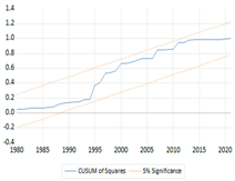 |
| OEt | CUSUM | 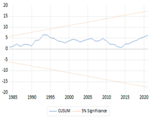 | 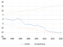 |
| OEt | CUSUMsq | 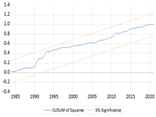 | 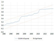 |
| GEt | CUSUM | 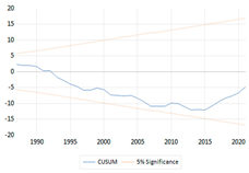 | 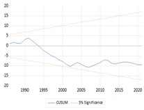 |
| GEt | CUSUMsq |  |  |
| GFEt | CUSUM |  | 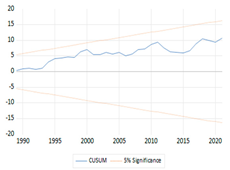 |
| GFEt | CUSUMsq | 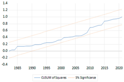 | 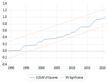 |
| CEt | CUSUM | 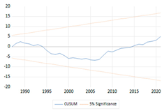 |  |
| CEt | CUSUMsq | 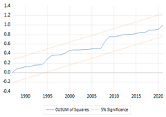 | 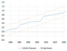 |
Disclaimer/Publisher’s Note: The statements, opinions and data contained in all publications are solely those of the individual author(s) and contributor(s) and not of MDPI and/or the editor(s). MDPI and/or the editor(s) disclaim responsibility for any injury to people or property resulting from any ideas, methods, instructions or products referred to in the content. |
© 2023 by the author. Licensee MDPI, Basel, Switzerland. This article is an open access article distributed under the terms and conditions of the Creative Commons Attribution (CC BY) license (https://creativecommons.org/licenses/by/4.0/).
Share and Cite
MDPI and ACS Style
Mahmood, H. The Determinants of Carbon Intensities of Different Sources of Carbon Emissions in Saudi Arabia: The Asymmetric Role of Natural Resource Rent. Economies 2023, 11, 276. https://doi.org/10.3390/economies11110276
AMA Style
Mahmood H. The Determinants of Carbon Intensities of Different Sources of Carbon Emissions in Saudi Arabia: The Asymmetric Role of Natural Resource Rent. Economies. 2023; 11(11):276. https://doi.org/10.3390/economies11110276
Chicago/Turabian StyleMahmood, Haider. 2023. "The Determinants of Carbon Intensities of Different Sources of Carbon Emissions in Saudi Arabia: The Asymmetric Role of Natural Resource Rent" Economies 11, no. 11: 276. https://doi.org/10.3390/economies11110276
Note that from the first issue of 2016, this journal uses article numbers instead of page numbers. See further details here.