Testing the Sustainability of Fiscal Policy during the Portuguese First Republic Using Stationary and Cointegration Tests

Abstract

The Portuguese First Republic (1910–1926) was marked by significant instability at the most diverse levels. With a special focus on the financial dimension of this period, the objective of this paper is to test the sustainability of the Portuguese fiscal policy, also referred to as the sustainability of public finances itself. The methodology involves testing the stationarity of public debt and budget balance and also the cointegration between state revenue and expenditure. The results obtained shows that the state’s intertemporal budgetary constraint was violated during the First Republic regime, which denotes unsustainability. This conclusion is justified by the existence of a non-stationary budget balance and the absence of cointegration between state revenue and expenditure. These results are manifestly different from those that have already been obtained for other Portuguese regimes, namely for the Estado Novo (1933–1974) and democracy (1974–present), where sustainability existed. This paper is yet another demonstration of how important it is to maintain control of state’s accounts. We hope that this paper can be useful to stimulate new research on Portuguese public finances and also on the important issue of fiscal policy sustainability.

1. Introduction

With the end of the monarchy, a new political regime emerged on 5 October 1910, in which the population placed enormous expectations. The First Republic (1910–1926), which emerged in a Europe characterised by monarchies, with the exception of France and Switzerland, presented alternative political and social principles that included the complete separation of church and state, widespread access to education, universal suffrage, a democracy without censorship, and no limitation to the free organisation and expression of opinion. However, many of these principles ended up not even being implemented (Telo 2010), and on the contrary, this regime failed to bring about the desired change. A state of permanent chaos lasted for 16 years, marked by enormous instability at the most diverse levels, not only political—with a total of 45 governments—but also social, economic, and financial. The First Portuguese Republic ended up falling early on—even though it already felt old—when a coup d’état was carried out by the military on 28 May 1926 (for more details on this regime, see also Oliveira Marques 1978, 2010; Rosas and Rollo 2009; Telo 2011; Martins and Duarte 2014).

With a special focus on the financial dimension, the objective of this paper is to test the sustainability of the fiscal policy in this specific period of Portugal’s history. It is important to clarify that, according to the literature, a sustainable fiscal policy implies that the ratio of debt converges to its initial level (Blanchard et al. 1990). This implies that the government needs to produce sufficient primary surpluses in the medium/long term to finance the accumulated debt (Chalk and Hemming 2000; European Central Bank 2011); this fiscal sustainability is synonymous of the ability of a government to sustain its policies in the long run without threatening the state’s solvency (European Commission 2017).

Therefore, we seek to answer the following fundamental questions: Can we consider that the political decision makers of this regime conducted the country’s fiscal policy responsibly? That is to say, was Portuguese fiscal policy sustainable in this specific period of 1910–1926? When compared with other periods (e.g., Estado Novo [New State], 1933–1974, and Democracy, 1974–present), what conclusions can we draw?1 To answer these questions, a set of important indicators relating to Portuguese public finances will be analysed, and econometric techniques usually used for this purpose will be carried out, namely stationarity and cointegration tests. This work could thus be of interest for all those who are not only dedicated to the study of Portuguese public finances but also for those who investigate the important issue of fiscal policy sustainability.

This paper is structured in five sections. After this introduction, Section 2 performs an analysis of the evolution of a set of relevant macroeconomic indicators. Section 3 presents the econometric methodology for testing the sustainability of fiscal policy. Section 4 discusses the results of the econometric tests, and, finally, Section 5 presents the main conclusions.

2. Brief Framework: The Portuguese Public Finances during the First Republic

At the beginning of the 20th century, Portugal was a shadow of its former power, having been humiliated by the British Ultimatum of 1890 and by a partial bankruptcy in 1892, both events which contributed to affect the credibility of the Portuguese monarchy (Ferraz 2023). It also had one of the most backward economies in Europe, characterised by low levels of economic development, as can be seen in

Table 1. GDP per capita in a set of European Countries 1901 and 1910.

	Real GDP per Capita (Constant 2011 International $), Year 1901	Real GDP per Capita (Constant 2011 International $), Year 1910
Austria	4565	5244
Belgium	5928	6478
Bulgaria	1722 *	1812
Denmark	4948	5906
Finland	2608	3038
France	4505	4726
Germany	4576	5337
Greece	1890	2592
Hungary	2681 **	3188
Italy	3317	3829
Netherlands	5483	6030
Norway	3271	3826
Poland	2700	2694
Portugal	2075	1957
Romania	641	784
Spain	2885	2823
Sweden	3406	4053
Switzerland	6399	8048
United Kingdom	7516	7718

Source: See Table A1 in Appendix A. * Data are missing for the year 1901, so this value reports to 1905. ** Data are missing for the year 1901, so this value reports to 1900.

.

Indeed, out of the 19 European nations considered in this table, only Bulgaria and Romania had a per capita GDP lower than that of Portugal in 1901. This was also a reality in 1910, the year that marked the end of the monarchy and the beginning of the Portuguese First Republic (1910–1926). In fact, it is possible to observe that Portuguese GDP per capita even shrank, in real terms, from 1901 to 1910.

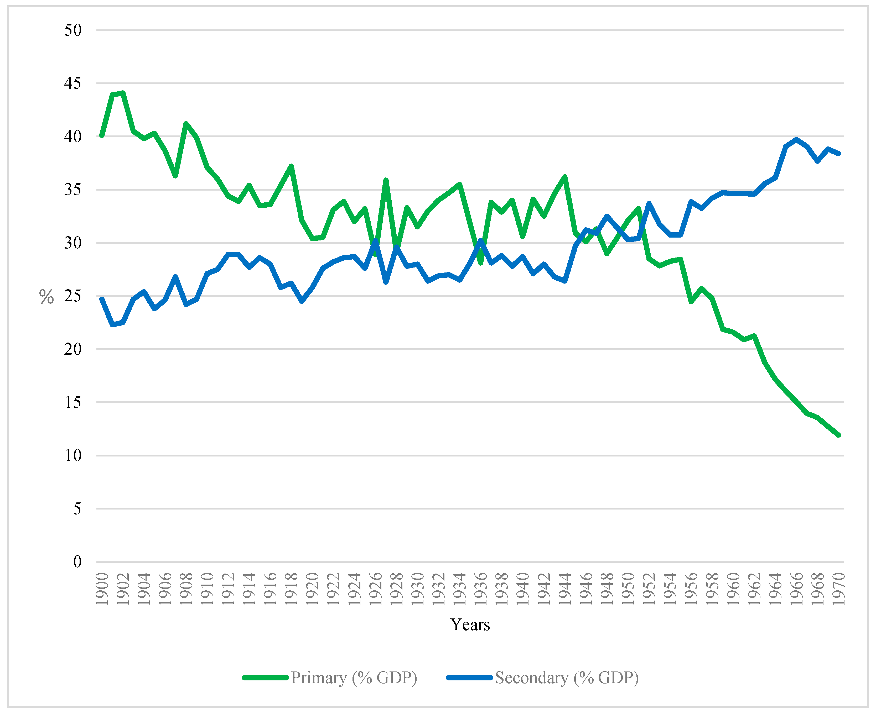
At that time, the primary sector had an extraordinarily high weight in the Portuguese economy, as can be seen in Figure 1. In fact, the secondary sector in Portugal would only surpass the weight of the primary sector decades later, during the Estado Novo regime—a time when Portugal underwent a strong industrialisation process.2

During the same period, Portugal was mostly an illiterate nation that was excessively dependent on foreign trade in terms of food supplies and energy (Pires 2011). It was in this context that Portugal entered the First World War (1914–1918) in 1916, after Germany’s declaration of war (Ferraz 2020b). Portugal’s desire to become an official belligerent existed right from the start of the First World War and was motivated by the following reasons: (1) defending its interests in Africa; (2) recovering the country’s external credibility; and (3) giving prestige to the young Republican regime whose legitimacy was still under question (Mata 2009; Serra 2009; Telo 2010; Ferraz 2023).

In this sense, the war could not have had worse repercussions for Portugal from the most diverse perspectives. From a financial point of view, and as can be seen in Figure 2, the conflict resulted in a sharp rise in Portuguese military spending, which attained 8% of GDP in the last year of the war, having been only 2% before the conflict.

The increase in military spending corresponded to an increase in budget deficits, which attained 8% of GDP, with the highest level occurring during the short period of the Portuguese First Republic. This was due to the fact that state revenues did not keep up with the sharp growth in expenses, which led to the derailment of public accounts, as can be seen in Figure 3.

In fact, Portugal experienced enormous difficulties in obtaining finance to pay for the increase in military spending. Due to the declaration of partial bankruptcy in 1892, and with the exception of a few small floating loans, the country was excluded from the international financial markets until after the Second World War (Mata and Valério 1998). Therefore, a large proportion of the deficits was financed through loans obtained from the Banco de Portugal [Bank of Portugal]—which at the time was the most relevant commercial bank in Portugal, with the exclusive right to issue currency—which increased the money supply.

As a result, inflation soared, with the escudo devaluing significantly against the British pound.3 The scarcity of essential goods on which Portugal, at the time, was heavily depended—such as wheat and also coal—also contributed to this inflationary process (Ferraz 2023). The prices of imports increased during the war, leading to hunger and the paralysis of important sectors in Portugal, which contributed to the aggravation of the Portuguese trade balance deficit, which can also be explained by the fall in the re-export trade of colonial products from Africa (Telo 2011).

In fact, the war resulted in a profound social and economic crisis for Portugal (Rosas 2009; Lains 2003; Mata and Valério 2003), with inflation remaining a problem for several years after this conflict ended. It is therefore relatively consensual that the First World War contributed decisively to the fall of the First Portuguese Republic.

It is worth noting that the First World War also resulted in a strong reduction in public debt as a percentage of GDP, despite the fact that the stock of public debt increased very significantly during that same period, as can be seen in Figure 4.

This reduction in public debt as a percentage of GDP was due to the strong nominal GDP growth, which was explained by the context of the high level of inflation. Indeed, while nominal GDP grew, on average, by 22% during the period of the First Republic, real GDP at 1914 prices (see Valério 2008, data) contracted on average by 0.1% per year during the same period.4 The literature on the relationship between inflation and debt is vast. For example, taking into account a sample of 19 advanced economies, Fukanaga et al. (2019) conclude that a 1 percentage point (pp) shock to inflation rate reduces the debt-to-GDP ratio by about 0.5 to 1 pp.

However, despite the sharp drop in the debt ratio, can we consider that the fiscal policies adopted were sustainable during this regime, and how should they be evaluated empirically?

3. Literature Review: Empirical Strategy

Whether budgetary policies are sustainable or not is a central question for macroeconomic analysis (Canofari et al. 2020b). For example, fiscal policy has the potential to influence economic growth and therefore the development of a country (Nguyen and Nguyen 2023; Shahini and Grabova 2023).5 In turn, fiscal policy sustainability—which is also referred to as public finances sustainability (European Commission 2017)—is a concept that is associated with solvency. A state is solvent if its intertemporal budget constraint is respected, that is to say, if the present value of its primary budget balances are sufficient to pay the public debt (Horne 1991; Chalk and Hemming 2000; Croce and Juan-Ramón 2003; European Central Bank 2011).

According to the literature, state budget constraint is the starting point for assessing the sustainability of budgetary policy which can be presented, in real terms, as follows:6

$$B_t-B_{t-1}=r_t·B_{t-1}+G_t-R_t,$$

(1)

where:

• G is primary expenses;
• R is state revenues;
• r is the real interest rate;
• B is the public debt stock.

Equation (1) means that the variation in the debt stock depends on the difference between expenses and revenues (for simplicity, we assume that other factors, in addition to these, are equal to zero). The previous equation can also be expressed as follows:

$$B_t=(1+r_t)·B_{t-1}+G_t-R_t$$

(2)

Assuming that the real interest rate is stationary—a hypothesis which is assumed in the literature—and considering $E_t$ as the primary expenditure plus real interest, with interest rates around r, we can obtain:

$$E_t+(1+r)·B_{t-1}=R_t+B_t,$$

(3)

from this last equation, an alternative formulation can be obtained:

$$B_{t-1}=\frac{1}{1+r}·(R_t-E_t)+\frac{B_t}{1+r},$$

(4)

using successive recursive substitutions, we obtain the following alternative formulation for the intertemporal budget constraint for an indefinite number of periods:

$$B_{t-1}={\sum }_{S=0}^{\infty }\frac{1}{(1+r{)}^{S+1}}·(R_{t+S}-E_{t+S})+\underset{S\to \infty }{\mathit{lim}} \frac{B_{t+S}}{(1+r{)}^{S+1}}.$$

(5)

Therefore, a sustainable fiscal policy needs to ensure that the public debt will have to tend towards zero in limit, as shown in the following equation:

$$\underset{s\to \infty }{\mathit{lim}} \frac{B_{t+S}}{(1+r{)}^{S+1}}=0$$

(6)

Public debt stock cannot increase indefinitely at a growth rate higher than the real interest rate. This implies that the state has to guarantee sufficient primary surpluses in the medium/long term to finance the accumulated debt:

$$B_{t-1}={\sum }_{S=0}^{\infty }\frac{1}{(1+r{)}^{S+1}}·(R_{t+S}-E_{t+S})$$

(7)

This algebraic development can also be carried out with the variables as a percentage of GDP. In this case, a sustainable fiscal policy implies that the debt-to-GDP ratio will have to tend towards zero in limit, thus converging to its initial level, while at the same time primary surpluses as a percentage of GDP will at least equal the value of the debt ratio at that initial moment (Blanchard et al. 1990; European Central Bank 2007).

Several econometric procedures, that have been widely used to test the sustainability of fiscal policy in various countries at different moments of time, all of which are based on the original work of Hamilton and Flavin (1986).7 Following Trehan and Walsh (1991) closely, we can consider that if the debt series is stationary, or at least I(1), then the condition expressed in Equation (6) will be respected. This procedure is conceptually equivalent to testing the order of integration of the budget balance series, which, in turn, must be I(0). Accordingly, the authors considered that in a context when the expected real interest rate is constant, the stationarity of the budget balance turns out to be a “necessary and sufficient” condition for the existence of a sustainable fiscal policy in a context where public debt will have to be at least I(1).

In turn, Hakkio and Rush (1991) proposed a complementary procedure that involves testing state revenues and expenses. This implies starting by rewriting Equation (7) in first differences:

$$∆B_t={\sum }_{S=0}^{\infty }\frac{1}{(1+r{)}^{S-1}}({∆R}_{t+S}-∆E_{t+S}),$$

(8)

Considering now, $S_t$ = $G_t$ + $r_t·B_{t-1}$, and assuming that ∆$B_t$ = $S_t$ − $R_t$, then we will have:

$$S_t-R_t={\sum }_{S=0}^{\infty }\frac{1}{(1+r{)}^{S-1}}({∆R}_{t+S}-∆E_{t+S})$$

(9)

Admitting that R and E are non-stationary series, although their first differences are, this means that also those S and R that are not stationary series need to be I(1) and must present a long-term equilibrium relation. Therefore, and after checking the order of integration of revenues and expenses (which must be the same), this procedure involves testing the following regression:

$$R_t=\mu +\beta S_t+u_t$$

(10)

There are two possibilities to take into account: (1) the null hypothesis in which R and S are not cointegrated; (2) the alternative hypothesis in which both I(1) have to be cointegrated. The procedure therefore involves testing the orders of integration of R and S, estimating a regression, and also testing the order of $\widehat{u}$, which must be I(0). In short, for a fiscal policy to be sustainable, it needs a stationary public debt in levels, I(0), or in its first differences, I(1), as well as a budget balance that also must be I(0), which is conceptually equivalent to the existence of cointegration between state revenues and expenses (where $\widehat{\beta }$ should be as close to 1 as possible).8

4. Results: Sustainability or Unsustainability?

We start by performing the necessary and usual unit root tests for the period of 1910–1926. We choose the ADF (Dickey and Fuller 1979) and PP (Phillips and Perron 1988) tests and, additionally, a unit root test with structural breaks (Eviews 2022 following Perron 1989). As suggested by Hakkio and Rush (1991), and as is usually described in the literature, we express all the variables as a percentage of GDP. Accordingly, p and s represent state revenues and expenses as a percentage of GDP, b is the public debt/GDP ratio, and d is the budget balance as a percentage of GDP in the financial years from 1910 to 1911 to 1925 to 1926. However, using a small sample, such as the one used in this study, means that the level of uncertainty that is always present in econometric tests increases (Gavilales 2019; Ferraz 2023).

The results of these tests are presented in

Table 2. Results of the unit root tests.

Variable	ADF	PP	Unit Root Tests with Structural Breaks	Global Conclusion
$p_t$	I(1)	I(1)	Neither I(0) nor I(1)	I(1) or above
$s_t$	I(1)	I(1)	I(1)	I(1)
$b_t$	I(1)	I(1)	I(1)	I(1)
$d_t$	I(1)	I(1)	I(1)	I(1)

Source: See Table A1 in Appendix A. Note: To consult the results of each of the tests, see Table A2, Table A3 and Table A4 in Appendix A.

, where it is possible to observe that s, b, and d are stationary series in their first differences I(1), with p also possibly being an I(1) series (only the unit root test with structural breaks presented a different conclusion).

From the outset, the non-stationarity of the budget balance ratio (d) is clearly an unfavourable result for the sustainability of fiscal policy/public finances. However, as the debt ratio (b) presented the result of I(1), we decided to continue to progress to the cointegration tests of revenues and expenses expressed as a percentage of GDP. We thus start by performing the two-step cointegration test, known as the Engle–Granger test (Engle and Granger 1987), which is in line with both the procedure proposed by Hakkio and Rush (1991) and our Equations (9) and (10).

The results are expressed in

Table 3. Results of the Engle–Granger cointegration test.

Step 1: Estimation of Cointegration Regression by the OLS Method
Result of Step 1: $\widehat{\beta }$ = 0.22 (0.27)
Step 2: Unit Root Tests for $\widehat{\mathit{u}}$
Tests	Result of Step 2
ADF	Non-stationary
PP	Non-stationary
Unit root tests with structural breaks	Non-stationary

Source: See Table A1 in Appendix A. Note 1: *, **, and *** represent the statistical significance of the regressor at the 10%, 5%, and 1% levels, respectively. The figures shown in brackets are standard errors. Note 2: For more details on the unit root tests, see Table A5 in Appendix A.

:

As can be seen, the estimated coefficient of β predicted in Equation (10) did not present statistical significance in the regression, and therefore should the first step fail, it is normal that the second also failed, that is that the estimated residuals ($\widehat{u}$) are not stationary. Therefore, according to this test, we found no cointegration between revenues and expenses.

In order to obtain a more robust conclusion, we also decided to perform the Johansen cointegration tests (Johansen 1988, 1991; Johansen and Juselius 1990). These new results are reported in

Table 4. Results of the Johansen cointegration tests.

Lags	Rank	Trace Test			Maximum Eigenvalue Test
		${\mathit{h}}_0$	${\mathit{h}}_1$	p-Value	${\mathit{h}}_0$	${\mathit{h}}_1$	p-Value
1	0	r = 0	r > 0	0.38	r = 0	r = 1	0.45
	1	r ≤ 1	r > 1	0.45	r = 1	r = 2	0.45

Source: See Table A1 in Appendix A. Note 1: r is the number of cointegration vectors. Note 2: *, **, and *** represent the rejection of the null hypothesis at the 10%, 5%, and 1% levels. The p-values were automatically computed by Gretl (2021). Note 3: The tests were performed with constant and no trend. The actual lag was chosen in order to optimise the Akaike Information Criterion (AIC), the Bayesian Information Criterion (BIC), and the Hannan–Quinn Information Criterion (HQC).

.

The results of these Johansen tests indicate that no cointegrating vectors were found, which confirms the results of the Engle–Granger test. In this sense, we can effectively conclude, with relative comfort, that there was no cointegration between the revenues and expenses during the period in question.

By analysing the set of results obtained, in the context of the literature, it is possible to conclude that despite the public debt ratio having decreased, due to the strong inflationary period, and that this variable is stationary in its first differences, the results relating to the budget balance (absence of stationarity) and revenue and expenditure (absence of cointegration) violates the state’s intertemporal budget constraint, which is synonymous of an unsustainable fiscal policy (or unsustainable public finances) during the Portuguese First Republic (1910–1926). This conclusion is quite different from those already obtained for other periods for which it was possible to conclude that there was sustainability, such as during the period between the Second World War (1939–1945) and the beginning of the 1970s (see Martins 2015), and also for Estado Novo, 1933–1974 (see Ferraz 2017), and Democracy, 1974–present (see Ferraz et al., forthcoming), regimes.

5. Conclusions

The First Republic (1910–1926) was a Portuguese political regime which was marked by enormous instability at the most diverse levels. It is relatively consensual that entry into the First World War (1914–1918) as a combatant during the first years of this regime had harsh and relatively prolonged consequences for Portugal, and that this was one of the main factors for its relatively short life.

From a financial point of view, budget deficits predominated, which were higher during the war owing to the increase in military expenditure. Given the enormous difficulties in obtaining finance, a large proportion of these deficits were financed through loans obtained from the Banco de Portugal, which increased the money supply. As a result, inflation soared, with the escudo devaluing significantly against the pound. The scarcity of essential goods on which Portugal was heavily dependent also contributed to this inflationary process. The prices of imports increased during the war, which, in turn, led to hunger and paralysis of important sectors. Indeed, inflation continued to be a problem after the war ended, which contributed to weakening the regime. However, this problem resulted in a sharp reduction in the public debt/GDP ratio, which was explained by the growth of nominal GDP, given that the debt stock grew at high rates.

By testing the sustainability of fiscal policy—which is also referred to in the literature as sustainability of public finances—during this troubled period, and by using econometric techniques which are usually used for this purpose, it was possible to conclude that the state’s intertemporal budgetary constraint was violated during the First Republic regime, which equates to unsustainability. This conclusion is justified by both the existence of a non-stationary budget balance and the absence of cointegration between state revenues and expenditures, despite the existence of the stationarity of the public debt/GDP ratio in its first differences in a context where the reduction in this ratio during most of the period in question was due to nominal GDP growth rates, which can be explained by considerable inflationary problems. However, a limitation must be recognised as, in effect, the use of a small sample (with only 16 observations) means that the level of uncertainty which is always present in this kind of applied exercise increases. As is understandable, this is justified by the short duration of the regime itself.

These results are different from those that have already been obtained for other Portuguese regimes, namely for the Estado Novo (1933–1974) and democracy (1974–present). Although the existing literature on the First Republic has already recognised the fact that during this regime, there was instability at the most diverse levels, this paper proves, for the first time and from an applied point of view, that in budgetary terms, there really was unsustainability regarding the conduct of budgetary policy by political decision makers, which enables us to conclude that Portuguese public finances were unsustainable at that time when evaluating this period as a whole (1910–1926).

This paper represents yet another demonstration of how important it is to maintain control of the state’s accounts. In fact, political decision makers must always conduct responsible policies and avoid running high deficits, while leaving public finances in a situation of unsustainability that would significantly aggravate the population. We also hope that this work can be useful for all those who research Portugal’s public finances, as well as the important issue of fiscal policy sustainability, and that it will thus stimulate the carrying out of new and interesting research.

References

- Afonso, Antonio. 2005. Fiscal Sustainability: The Unpleasant European Case. FinanzArchiv 61: 19–44. [Google Scholar] [CrossRef]
- Afonso, António, Emanuel Reis Leão, Dilson Tiny, and Diptes C. P. Bhimjee. 2022. Sustentabilidade fiscal nas economias PALOP. Notas Económicas 55: 55–70. [Google Scholar] [CrossRef] [PubMed]
- Blanchard, Olivier J., Jean-Claude Chouraqui, Robert Hagemann, and Nicola Sartor. 1990. The Sustainability of Fiscal Policy: New Answers to an Old Question. OECD Economic Studies 15: 7–36. [Google Scholar]
- Canofari, Paolo, Alessandro Piergallini, and Giovanni Piersanti. 2020a. Assessing sovereign debt sustainability using a wealth-based fiscal indicator. Economics Bulletin 40: 2677–88. [Google Scholar]
- Canofari, Paolo, Giancarlo Marini, and Alessandro Piergallini. 2020b. Financial Crisis and Sustainability of US Fiscal Deficit: Indicators or Tests? Journal of Policy Modeling 42: 192–04. [Google Scholar] [CrossRef]
- Chalk, Nigel, and Richard Hemming. 2000. Assessing Fiscal Sustainability in Theory and Practice. IMF Working Paper 00/81. Washington, DC: IMF. [Google Scholar]
- Croce, Enzo, and V. Hugo Juan-Ramón. 2003. Assessing Fiscal Sustainability: A Cross-Country Comparison. IMF Working Paper, 03/145. Washington, DC: IMF. [Google Scholar]
- Dickey, David, and Wayne Fuller. 1979. Distribution of the Estimators for Time Series Regressions with a Unit Root. Journal of the American Statistical Association 74: 427–31. [Google Scholar]
- Engle, Robert, and Clive Granger. 1987. Co-Integration and error correction: Representation, estimation, and testing. Econometrica 55: 251–76. [Google Scholar] [CrossRef]
- European Central Bank. 2007. Assessing Fiscal Soundness—Theory and Practice. Occasional Paper Series, 56; Frankfurt: European Central Bank. [Google Scholar]
- European Central Bank. 2011. Ensuring Fiscal Sustainability in the Euro Area. European Central Bank, Monthly Bulletin. Frankfurt: European Central Bank, pp. 61–77. [Google Scholar]
- European Commission. 2017. European Semester Thematic Factsheet—Sustainability of Public Finances. Available online: https://commission.europa.eu/system/files/2020-06/european-semester_thematic-factsheet_public-finance-sustainability_en_0.pdf (accessed on 23 September 2023).
- Eviews. 2022. Eviews Version 12 for Econometric Analysis. Available online: https://www.eviews.com/home.html (accessed on 5 December 2022).
- Ferraz, Ricardo. 2017. The Sustainability of Portuguese Fiscal Policy in the Period of the Estado Novo, 1933–1974. The Journal of European Economic History 46: 37–68. [Google Scholar]
- Ferraz, Ricardo. 2018. Have Public Finances in the OECD Are Been Sustainable? Economics and Business 32: 36–50. [Google Scholar] [CrossRef]
- Ferraz, Ricardo. 2020a. The Portuguese Development Plans in the Postwar Period: How Much Was Spent and Where? Investigaciones de Historia Económica—Economic History Research 16: 45–55. [Google Scholar]
- Ferraz, Ricardo. 2020b. Grande Guerra e Guerra Colonial—Custos para os Cofres Portugueses. Lisboa: Edições Sílabo. [Google Scholar]
- Ferraz, Ricardo. 2022a. The Financial Costs of the Portuguese Colonial War, 1961–1974: Analysis and Applied Study. Revista de Historia Economica—Journal of Iberian and Latin American Economic History 40: 243–72. [Google Scholar] [CrossRef]
- Ferraz, Ricardo. 2022b. Os Planos de Fomento do Estado Novo—Quantificação e Análise. Lisboa: Edições Sílabo. [Google Scholar]
- Ferraz, Ricardo. 2023. The Portuguese budgetary costs with First World War: A comparative perspective. European Review of Economic History 27: 278–301. [Google Scholar] [CrossRef]
- Ferraz, Ricardo, António Portugal Duarte, and Joaquim Miranda Sarmento. Forthcoming. The Sustainability of Portuguese Fiscal Policy in Democracy, 1974–2020. Paper Currently Submitted to an International Journal. Unpublished Paper.
- Fukanaga, Ichiro, Takuji Komatsuzaki, and Hideaki Matsuoka. 2019. Inflation and Public Debt Reversals in Advanced Economies. IMF Working Papers, 2019/297. Washington, DC: International Monetary Fund (IMF). [Google Scholar]
- Gavilales, John. 2019. Low sample size and regression: A Monte Carlo approach. Journal of Applied Sciences 1: 22–44. [Google Scholar]
- Gretl. 2021. Gnu Regression, Econometrics and Time-Series Library. Available online: http://gretl.sourceforge.net/ (accessed on 30 October 2021).
- Hakkio, Craig, and Mark Rush. 1991. Is the budget deficit “too large? Economic Inquiry 29: 429–45. [Google Scholar] [CrossRef]
- Hamilton, James, and Marjorie Flavin. 1986. On the limitations of government borrowing: A framework for empirical testing. American Economic Review 76: 808–19. [Google Scholar]
- Hasanov, Fakhri, Fuad Mammadov, and Nayef Al-Musehel. 2018. The effects of Fiscal Policy on Non-oil Economic Growth. Economies 6: 27. [Google Scholar] [CrossRef]
- Horne, Jocelyn. 1991. Indicators of Fiscal Sustainability. IMF Working Paper, 91/5. Washington, DC: International Monetary Fund (IMF). [Google Scholar]
- Instituto Nacional de Estatística and Banco de Portugal. 2021. Séries Longas para a Economia Portuguesa 2020 (SLEP 2020). National Statistics Institute and Bank of Portugal. Available online: https://www.ine.pt/xportal/xmain?xpid=INE&xpgid=ine_publicacoes&PUBLICACOESpub_boui=536285836&PUBLICACOESmodo=2 (accessed on 1 December 2022).
- Johansen, Søren. 1988. Statistical Analysis of Cointegragtion Vectors. Journal of Economic Dynamics and Control 12: 231–54. [Google Scholar] [CrossRef]
- Johansen, Søren. 1991. Estimation and Hypothesis Testing of Cointegration Vectors in Gaussian Vector Autoregressive Models. Econometrica 59: 1551–80. [Google Scholar] [CrossRef]
- Johansen, Søren, and Katarina Juselius. 1990. Maximum likelihood estimation and inference on cointegration with applications to the demand for money. Oxford Bulletin of Economics and Statistics 52: 169–210. [Google Scholar] [CrossRef]
- Kalyoncu, Huseyin. 2005. Fiscal policy sustainability: Test of intertemporal borrowing constraints. Applied Economics Letters 12: 957–62. [Google Scholar] [CrossRef]
- Lains, Pedro. 2003. Os Progressos do Atraso—Uma Nova História Económica de Portugal. Lisboa: ICS. [Google Scholar]
- Léonard, Yves. 1998. Salazarismo e Fascismo. Sintra: Inquérito Colecção. [Google Scholar]
- Malla, Manwar Hossein, and Pairote Pathranarakul. 2022. Fiscal Policy and Income Inequality: The Critical Role of Institutional Capacity. Economies 10: 115. [Google Scholar] [CrossRef]
- Martins, Nuno Ricardo Sampaio Veiga Ferraz. 2015. As Finanças Públicas Portuguesas no Período de Ouro de Crescimento da Economia Portuguesa, 1947–1974: Análise e Estudo Aplicado. Ph.D. dissertation, ISEG, Universidade de Lisboa, Lisboa, Portugal. [Google Scholar]
- Martins, Nuno Ferraz, and António Portugal Duarte. 2014. The Public Finances and the Economic Growth in the First Portuguese Republic. Economic Analysis 47: 59–75. [Google Scholar]
- Mata, Eugénia. 1993. As Finanças Públicas Portuguesas da Regeneração à Primeira Guerra Mundial. Lisboa: Banco de Portugal. [Google Scholar]
- Mata, Eugénia. 2009. A Política Financeira. In História da Primeira República Portuguesa. Edited by Fernando Rosas and Maria Rollo. Lisboa: Tinta-da-China, pp. 191–203. [Google Scholar]
- Mata, Eugénia, and Nuno Valério. 1998. Dívida pública externa e crescimento económico em Portugal (1830–1914). Notas Económicas 11: 120–30. [Google Scholar]
- Mata, Eugénia, and Nuno Valério. 2003. História Económica de Portugal—Uma Perspectiva Global. Lisbon: Editorial Presença. [Google Scholar]
- Mateus, Abel. 2013. Economia Portuguesa: Evolução no Contexto Internacional 1910–2013. Cascais: Principia. [Google Scholar]
- Nguyen, Dung Xuan, and Trung Dung Nguyen. 2023. The relationship of Fiscal Policy and Economic Cycle: Is Vietnam Different? Journal of Risk and Financial Management 16: 281. [Google Scholar] [CrossRef]
- Oliveira Marques, António Henrique de. 1978. História da Primeira República. Lisboa: Iniciativas Editoriais. [Google Scholar]
- Oliveira Marques, António Henrique de. 2010. A Primeira República Portuguesa. Lisboa: Texto. [Google Scholar]
- Pereira, Paulo Trigo, António Afonso, Manuela Arcanjo, and José Carlos Gomes Santos. 2005. Economia e Finanças Públicas. Lisboa: Escolar Editora. [Google Scholar]
- Perron, Pierre. 1989. The Great Crash, the Oil Price Shock, and the Unit Root Hypothesis. Econometrica 57: 1361–401. [Google Scholar] [CrossRef]
- Phillips, Peter, and Pierre Perron. 1988. Testing for a Unit Root in Time Series Regression. Biometrika 75: 335–46. [Google Scholar] [CrossRef]
- Phillips, Peter C. B., and Donggyu Sul. 2007. Transition Modeling and Econometric Convergence Tests. Econometrica 75: 1771–885. [Google Scholar] [CrossRef]
- Piergallini, Alessandro, and Michele Postigliola. 2020. Evaluating the sustainability of Italian public finances. The North American Journal of Economics and Finance 53: 101180. [Google Scholar] [CrossRef]
- Pires, Ana Paula. 2011. Portugal e a I Guerra Mundial—A República e a Economia de Guerra. Sintra: Caleidoscópio. [Google Scholar]
- Rosas, Fernando. 1994. O Estado Novo 1926–1974. In História de Portugal, 7. Edited by José Mattoso. Lisboa: Círculo de Leitores. [Google Scholar]
- Rosas, Fernando. 2001. O Salazarismo e o Homem Novo: Ensaio sobre o Estado Novo e a Questão do Totalitarismo. Análise Social 35: 1031–54. [Google Scholar]
- Rosas, Fernando. 2009. A República e a Grande Guerra. In História da Primeira República Portuguesa. Edited by F. Rosas and Maria Rollo. Lisbon: Tinta-da-China, pp. 247–48. [Google Scholar]
- Rosas, Fernando, and Maria Rollo. 2009. História da Primeira República. Lisboa: Tinta da China. [Google Scholar]
- Serra, João. 2009. A evolução política (1910–1917). In História da Primeira República Portuguesa. Edited by Fernando Rosas and Maria Rollo. Lisbon: Tinta-da-China, pp. 93–148. [Google Scholar]
- Shaheen, Rozina. 2019. Impact of Fiscal Policy on Consumption and Labor Supply under a Time-Varying Structural VAR Model. Economies 7: 57. [Google Scholar] [CrossRef]
- Shahini, Ledjon, and Perseta Grabova. 2023. Economic role of Government Budget Revision in the Presence of COVID-19. Economies 11: 118. [Google Scholar] [CrossRef]
- Telo, António José. 2010. Primeira República I—Do Sonho à Realidade. Lisboa: Editorial Presença. [Google Scholar]
- Telo, António José. 2011. Primeira República II—Como Cai um Regime. Lisboa: Editorial Presença. [Google Scholar]
- Tendengu, Simbarashe, Forget Mingiri Kapingura, and Asrat Tsegaye. 2022. Fiscal Policy and Economic Growth in South Africa. Economies 10: 204. [Google Scholar] [CrossRef]
- The Maddison Project. 2020. Maddison Project Database, Version 2020—Bolt J, Van Zanden J. Available online: https://www.rug.nl/ggdc/historicaldevelopment/maddison/releases/maddison-project-database-2020 (accessed on 8 August 2023).
- Torgal, Luís Reis. 2009. Estados Novos, Estado Novo. Coimbra: Universidade de Coimbra. [Google Scholar]
- Trehan, Bhrat, and Carl Walsh. 1991. Testing Intertemporal Budget Constraints: Theory and Applications to U.S. Federal Budget and Current Account Deficits. Journal of Money, Credit and Banking 23: 206–23. [Google Scholar] [CrossRef]
- Valério, Nuno. 1994. As Finanças Públicas Portuguesas Entre as Duas Guerras Mundiais. Lisboa: Edições Cosmos. [Google Scholar]
- Valério, Nuno. 2008. Avaliação do Produto Interno Bruto de Portugal. GHES Working Paper Study, 34. Lisboa: Centre of Research into Economic and Social History (GHES)—Lisbon School of Economics & Management (ISEG), Universidade de Lisboa. [Google Scholar]
Figure 1.
The primary and secondary sectors of Portugal as a percentage of GDP, 1900 to 1970. Source and notes: See Table A1 in Appendix A.
Figure 2.
Military expenditure and budget balance in Portugal (as a percentage of GDP), 1900–1901 to 1925–1926. Source and notes: See Table A1 in Appendix A.
Figure 3.
State revenue and expenditure as a percentage of GDP, 1900–1901 to 1925–1926. Source and notes: See Table A1 in Appendix A.
Figure 4.
Portuguese public debt, 1901 to 1926. Source: See Table A1 in Appendix A.