
Do Local Fiscal Expenditures Promote the Growth of Profit-Seeking Enterprise Numbers in Neighboring Areas?


1
Department of Public Finance and Taxation, National Kaohsiung University of Science and Technology, Kaohsiung 807, Taiwan
2
Business Intelligence School, National Kaohsiung University of Science and Technology, Kaohsiung 807, Taiwan
3
Graduate Institute of Tourism Management, National Kaohsiung University of Hospitality and Tourism, Kaohsiung 812, Taiwan
*
Author to whom correspondence should be addressed.
Economies 2022, 10(2), 34; https://doi.org/10.3390/economies10020034
Submission received: 6 November 2021
/
Revised: 14 December 2021
/
Accepted: 26 January 2022
/
Published: 28 January 2022
(This article belongs to the Special Issue Challenges in Environmental and Resource Economics)
Abstract
:In order to allocate resources and formulate policies effectively, governments and enterprises often need accurate geographical information on profit-seeking enterprises. This study explores the impact of local fiscal expenditure and environmental regulation on the number of profit-seeking enterprises in Taiwan’s counties and cities from the perspective of spatial econometrics, and analyzes data from 2001 to 2019. After comparing the explanatory power differences of various spatial econometric models, the spatial Durbin model, with spatial and time fixed effects, was used to explore the direct effect on the number of local profit-seeking enterprises, and the spillover effect of the number of local profit-seeking enterprises in different geographical locations on neighboring regions, especially the spatial spillover effect of local fiscal expenditure and labor and environmental regulations. This paper discusses the decision-making choices of local government regarding the competition strategy of environmental regulation, and finally provides the policy implications for the government as a reference.
1. Introduction
The establishment of a profit-seeking enterprise can affect the economic development of the place where the enterprise is located. To attract companies and manufacturers to invest and set up factories, local governments often introduce many preferential policies and investment promotion measures. Tiebout (1956) proposed the “vote by feet” theory, suggesting that, under normal circumstances, there would be more population inflow in places that can effectively provide public goods and services that meet their consumption preferences; on the contrary, places that cannot effectively provide these products and services would face population outflow. The “vote by feet” theory revises the traditional notion that public finance leads to market failure and introduces the spatial concept into the financial theory. In this view, population mobility is affected not only by public expenditure, but also by the burden of rents and taxes.
It is worth discussing whether enterprises will invest and set up factories in the right places to drive economic growth, as part of the migration described by the “vote by feet” theory. This study attempts to explore the growth in the number of profit-seeking enterprises in various regions from the perspective of the spatial effect of fiscal expenditure, which has been seldom discussed in past studies. First, the relationship between fiscal expenditure and economic growth has been the focus of many scholars (Barro 1990; Easterly and Rebelo 1993; Helms 1985; Lin and Song 2002). For example, Arrow and Kurz (2011) discussed the relationship between fiscal expenditure and economic growth in the framework of neoclassical growth theory and, subsequently, this research topic attracted the attention of many scholars. Barro (1990) was the first to introduce fiscal expenditure into the production function. In this way, economic growth not only depends on the changes of production factors, such as capital accumulation and labor input, but also fiscal expenditure, which is regarded as an accumulative input of production factors. Boarnet (1998) suggested that the more complete a region’s infrastructure is, the more attractive it will be to neighboring regions’ capital, labor, and other factors of production. Through empirical analysis, Pereirã and Roca-Sagalés (2003) and Cohen and Morrison Paul (2004) found that public expenditure in a region, especially infrastructure construction, would have a positive spatial spillover effect on the economic growth of neighboring regions. Therefore, as a reflection of local fiscal capacity, local fiscal expenditure not only has a direct or indirect impact on the endowment and flow of production factors, such as labor, capital, technology, and information, but also has an important external effect on the operating environment of enterprises. This will naturally affect the growth in the number of profit-seeking enterprises.
Second, as far as the spatial dependence of the place of business of profit-seeking enterprises is concerned, the business or establishment behavior or phenomenon in the spatial geographical location does not exist independently, but has some spatial correlation with the phenomenon in the adjacent spatial geographical location. The distribution of profit-seeking enterprises has certain spatial rules, and the number of profit-seeking enterprises in different spatial geographical locations is affected by the local and neighborhood effect. Since the 1990s, spatial characteristics in the process of economic growth have been gradually examined by scholars. Bernat (1996) pointed out that there are spatial correlation and spatial spillover effects in the process of economic growth, and he was one of the early scholars who focused on spatial dependence in economic development. Rey and Montouri (1999) tested the spatial dependence, spatial heterogeneity and spatial convergence of economic development from the perspective of the neoclassical research, and found that ignoring the spatial effect of regional economic development would lead to the deviation of empirical results. This is because an important premise of traditional econometric models is to assume that the research objects are independent of each other, which is obviously inconsistent with reality. Traditional econometric models assume that spatial items are uncorrelated and homogenous, and model estimates are mostly made with the ordinary least squares (OLS) method. Ignoring spatial effects causes the biases commonly seen in these models. As a result, the estimations and inferences are not adequately robust, and hence fall short of the required explanatory power (LeSage and Pace 2009). The traditional econometric model has limitations in the analysis of spatial relations and numerical values; that is, it lacks the viewpoint of spatial effects, and it is difficult to reflect the distribution and change in the establishment of profit-seeking enterprises in different regions.
The spatial distribution pattern of the number of profit-seeking enterprises is the basis for studying the spatial structure of regional economic development, while the number of profit-seeking enterprises in different regions may have spatial autocorrelation. However, there are relatively few studies on spatial measurement on this topic. This study will bridge the gap between previous studies. The research objectives of this paper are as follows. (1) As Taiwan’s economy has grown steadily, the number of profit-seeking enterprises has been on a gradual rise. This study examined the spatial autocorrelation and distribution of profit-seeking enterprises in different the cities and counties of Taiwan, and the subsequent findings can serve as a reference for the establishment, operation, and investment of companies or manufacturers. (2) A comparison was performed on the explanatory power of multiple quantitative spatial econometric models, including the spatial autoregressive model (SAR), spatial error model (SEM), and spatial Durbin model (SDM). This study conducted its analysis by using the best model. (3) The fiscal spending factors that influence the number of profit-seeking enterprises include general government expenditures, economic development expenditures, expenditures on education, science, and culture, and expenditures on community development and environmental protection. The environmental condition factors that influence the number of profit-seeking enterprises include the net amount of tax collected, labor force participation rates, the number of lighting users, the proportion of employees with a junior college or higher education, and the percentage of employees aged from 25 to 44. This study examined the direct impact of the fiscal spending and environmental conditions in local cities and counties on the number of local profit-seeking enterprises. It also explored the spatial spillovers effects of the fiscal spending and environmental conditions in local cities and counties on the number of profit-seeking enterprises in adjacent cities and counties. (4) Different types of environmental conditions, as competitive strategies by local city/county governments, were also explored. The findings provide a reference for policymaking for local city/county governments.
2. Literature Review
Tobler (1970) proposed the First Law of Geography (Tobler’s First Law or Tobler’s First Law of Geography (TFL)): everything is related to everything else, but near things are more related than distant things. The First Law of Geography is concerned with the correlation of variables in different spatial geographies. This phenomenon is called spatial dependency or spatial autocorrelation.
Cliff and Ord (1973) mentioned the measurement of spatial autocorrelation, which mainly measures the values represented by adjacent spatial units (such as counties or states). If the values are similar, it means that there is spatial autocorrelation. Goodchild (1987) indicated that spatial autocorrelation quantifies the potential spatial dependence of geographical phenomena and describes the similarity between the phenomena in the region and other neighboring regions to identify the spatial aggregation. Sokal et al. (1988) proposed that spatial autocorrelation means to test the spatial differences between spatial unit variables and adjacent spatial variables. According to Anselin (1988), spatial autocorrelation refers to the potential spatial dependence of geographical phenomena, and it describes the spatial similarity between the region of a particular phenomenon and other neighboring regions by means of quantization, so as to identify the spatial aggregation characteristics. Therefore, the essence of spatial autocorrelation is to discuss the correlation between “local area” and “adjacent area”; that is, to discuss the influence degree of the “neighborhood effect”, and to explore the possible influence mechanism of producing a spatial neighborhood effect (Anselin 2003; Goodchild et al. 2000; Morenoff and Sampson 1997).
Phenomena in space are not independent. Due to the similarity of the economic conditions and the social and cultural conditions between neighboring regions, the economic radiation of population transfer, industrial development, resource accumulation, and factor flow leads to the obvious spatial agglomeration of neighboring regions. When the observed area has a high degree of similarity with its neighboring regions, it is likely to have a contagion or diffusion effect, which is called a spatial overflow effect. The development of regional economy is influenced by spatial factors, and spatial spillover is an important part of regional economic development.
Previous studies used the spatial econometric model for fiscal expenditure (Carruthers and Úlfarsson 2008; De Siano and D’Uva 2017; He et al. 2018; Jiang et al. 2020; Oyun 2017; Pan et al. 2020; Que et al. 2018; Tyrrell and Johnston 2009; Wang et al. 2021; Wu and Zhu 2021; Zhang et al. 2019). For example, Tyrrell and Johnston (2009) studied the impact of tourism growth on municipal income and expenditure in 21 cities under the jurisdiction of New London County, Connecticut, from 1993 to 2002. Oyun (2017) explored the interstate spillover effects of Medicaid expenditures in 50 states on home-and-community-based services (HCBS) from 2000 to 2010, and examined the relationship between fiscal decentralization and public expenditures. De Siano and D’Uva (2017) studied the spillover effect of fiscal decentralization and the public expenditure of local governments in Italy from 1996 to 2010. Que et al. (2018) discussed the spillover effect of fiscal decentralization on local public goods supply in 31 provinces of China from 1994 to 2013. He et al. (2018) used a spatial econometric model to study the determinants of company productivity and spatial spillover effects in China’s electric apparatus industry from 1999 to 2007, in which public expenditure was an important factor. In the past, the spatial econometric model was used to explore the theory of “vote by feet”. For example, Cheng and Pu (2017) studied the stable relationship between the effective tax rate and China’s economic growth from the perspective of spatial econometrics through the panel data of 31 Chinese provinces from 2007 to 2013. There are also studies on the factors influencing the employment growth of high-tech SMEs (Fingleton et al. 2004).
3. Methodology
3.1. Setting of the Spatial Econometric Model
The definitions and descriptions of dependent and independent variables in the empirical models are as follows:
Number of profit-seeking enterprises (NPSEi(j),t): This refers to the number of profit-seeking enterprises in the county (or city) i (j) in Taiwan in the t-th year. It is the number of companies registered for profit enterprise tax registration according to Article 28, Chapter 5 of the Value-added Tax and Non-value-added Tax Law.
General government expenditure (TWD million; New Taiwan Dollars) (GGEit): This refers to the general government expenditure of the ith county or city in Taiwan in the tth year. It is the expenditure of the county or city on the exercise of government power, administration, civil affairs, and finance (excluding police expenditure).
Economic development expenditure (TWD million) (EDEit): This refers to the economic development expenditure of the ith county or city in Taiwan in the tth year. It is the expenditure of the county or city on agriculture, industry, transportation, and other economic services.
Expenditure on education, science, and culture (TWD million) (EESCit): This refers to the education, science, and culture expenditure of the ith county or city in Taiwan in the tth year. It is the expenditure on education, science, and culture, and other undertakings and subsidies.
Expenditure on community development and environmental protection (TWD million) (ECDEPit): This refers to the expenditure for community development and environmental protection of the ith county or city in Taiwan in the tth year. It is the expenditure of a county or city for community development, environmental protection, and other undertakings and subsidies.
Net amount of tax collected (TWD thousand) (NATCit): This refers to the net amount of tax collected of the ith county or city in Taiwan in the tth year. The net amount of tax collected refers to the amount of tax collected in the current year minus the amount of tax refunds. The current year or previous years are included.
Number of lighting users (NLUit): This refers to the number of lighting users of the ith county or city in Taiwan in the tth year. It is the number of users of electricity for flat-rate lighting and metered lighting (including business and non-business users) of the Taiwan Power Company.
Labor force participation rate (%) (LFPRit): This refers to the percentage of the labor force of the ith county or city in Taiwan in the tth year in the population over 15 years old. Labor force refers to the working population over the age of 15, including the employed and the unemployed. The formula is (number of labor force/number of population over 15 years old) × 100.
Proportion of employees with a junior college or higher education (%) (PEEit): This refers to the percentage of the employees with a junior college or higher education of the ith county or city in Taiwan in the tth year in the total employment. The formula is (the number of the employees with a junior college or higher education/the total number of the employed people) × 100.
Percentage of employees aged 25 to 44 (%) (PEAit): This refers to the percentage of employees aged 25 to 44 in total employment in the first year of the ith county and city of Taiwan. The formula is (number of employees aged 25–44/total number of employees) × 100.
Panel data analysis can control the differences between cross-sectional individuals, reduce the collinearity among variables, adjust the autocorrelation of variables in time series analysis, and reduce the risk of bias derived from the measurement model. All kinds of economic activities are related in spatial geography, and with the development of the economy, they are more closely related in space. For simplification purposes, the intercept term is included in the matrix of independent variables, and the model in this study is written in matrix form. The empirical model in this study is as follows:
where denotes NPSEi(j),t, while is the spatial weighting matrix used to measure spatial correlation between geographical counties (cities), and is the vector of spatial lag coefficient and the spatial autocorrelation coefficient of the dependent variable. It reflects the direction and degree of the influence of the dependent variable () in the neighboring region on the dependent variable () of the region; that is, the influence of the dependent variable () of the region with spatial correlation on the dependent variable () of the region. By verifying the spatial lag coefficient (), we can further explore the spillover effect of the neighboring region on this region. When significantly differs from zero, this means that there is indeed a spatial relation with the neighboring region. The value of reflects the degree of interaction between regions, such as spatial diffusion or spatial spillover; is the spatial autocorrelation matrix of the dependent variable, which is an endogenous variable. It represents the influence of in region j adjacent to region i on in region i.
is the vector of coefficients to be estimated, which represents the original effect of the independent variable vector , which consists of GGEit, EDEit, EESCit, ECDEPit, NATCit, LFPRit, NLUit, PEEit, and PEAit. Therefore, our independent vector is .
reflects the original influence of each independent variable on , and is the coefficient vector to be estimated, which is the spatial autocorrelation coefficient of the independent variable. It reflects the influence of all the independent variables in the neighboring regions on in the region. A positive indicates that the neighborhood effect has a positive effect on the dependent variable , and that there is spillover effect between the neighboring regions, while a negative represents that there is a competition effect among the neighboring regions. is the matrix of the spatial autocorrelation terms of the independent variables, which represents the spatial effect of all independent variables and shows the influence of all independent variables in the neighboring areas on in region i. is the spatial (individual) effect, which is the individual effect of county (city) i, and is an independent and identically distributed random error term and a spatial autocorrelation error term.
In order to address the problem of inflation, this study takes the deflated consumer price index (CPI) as a real variable in each nominal variable of fiscal expenditures, excluding the impact of inflation on fiscal expenditure measurement. Among the variables, general government expenditure (GGEit), economic development expenditure (EDEit), expenditure on education, science, and culture (EESCit), expenditure on community development and environmental protection (ECDEPit), the net amount of tax collected (NATCit), and other nominal variables are deflated according to the CPI to remove the impact of inflation factors. For example: Nominal General Government Expenditure ÷ CPI × 100 = Real General Government Expenditure.
3.2. Data and Sample
This paper takes the data of 22 counties and cities in Taiwan for 19 years from 2001 to 2019 as samples. The codes and names of counties and cities in Taiwan are shown in Table 1. The data are mainly from the Key Statistical Index Inquiry System on Counties and Cities, under the National Statistics Website of the Republic of China.
3.3. Spatial Weight Matrix
The spatial weight matrix needs to be considered before constructing the spatial econometric model. The spatial weight matrix is the premise and foundation of spatial econometric analysis using exploratory spatial data analysis (ESDA). A binary symmetrical spatial weight matrix is usually defined to express the spatial neighborhood relation of n locations.
There are three methods to identify the adjacency of spatial units: rook contiguity, bishop contiguity, and queen contiguity. Rook contiguity refers to the contact between two spatial boundaries, bishop contiguity refers to the diagonal contiguity, and queen contiguity refers to contacts on the edge or diagonal (Sawada 2004). This research used the queen contiguity to define spatial adjacencies.
There are various rules for establishing a spatial weight matrix. Among them, a binary adjacency space weight matrix based on adjacency rules and distance rules is commonly used. This study used adjacency rules, which were defined as:
There are three island counties in Taiwan, and there is no adjacency relationship between these island counties and other counties; therefore, they exhibited a value of 0.
4. Results
4.1. Descriptive Statistics
4.2. Test of Spatial Autocorrelation
Before spatial econometric analysis, it is necessary to test whether the dependent variable has spatial autocorrelation. If the dependent variable has spatial autocorrelation, it is reasonable to add spatial geography factors. The detection of spatial autocorrelation can definitely analyze spatial relations (concentration, random, and dispersion). Spatial autocorrelation mainly includes global spatial autocorrelation and regional spatial autocorrelation. Among the various spatial autocorrelation indicators, Moran’s statistical power is the best (Walter 1992), thus making it the most widely used spatial autocorrelation indicator (Cliff and Ord 1973, 1981). The closer the value of Moran’s I approaches 1, the more it indicates that the positive spatial autocorrelation degree is stronger, and the closer the value approaches −1, the stronger the negative spatial autocorrelation degree is. According to Table 4, all the values of Moran’s I reach the significance level of 0.05, indicating that the number of profit-seeking enterprises in all counties and cities from 2001 to 2019 has a significant positive spatial autocorrelation. It is therefore suitable to use the spatial econometric model in this study. The trend chart of spatial autocorrelation is shown in Figure 1. Moran’s I in the past 19 years has roughly shown a decreasing trend year by year, indicating that the distribution of the number of profit-seeking enterprises in Taiwan’s counties and cities is less and less concentrated.
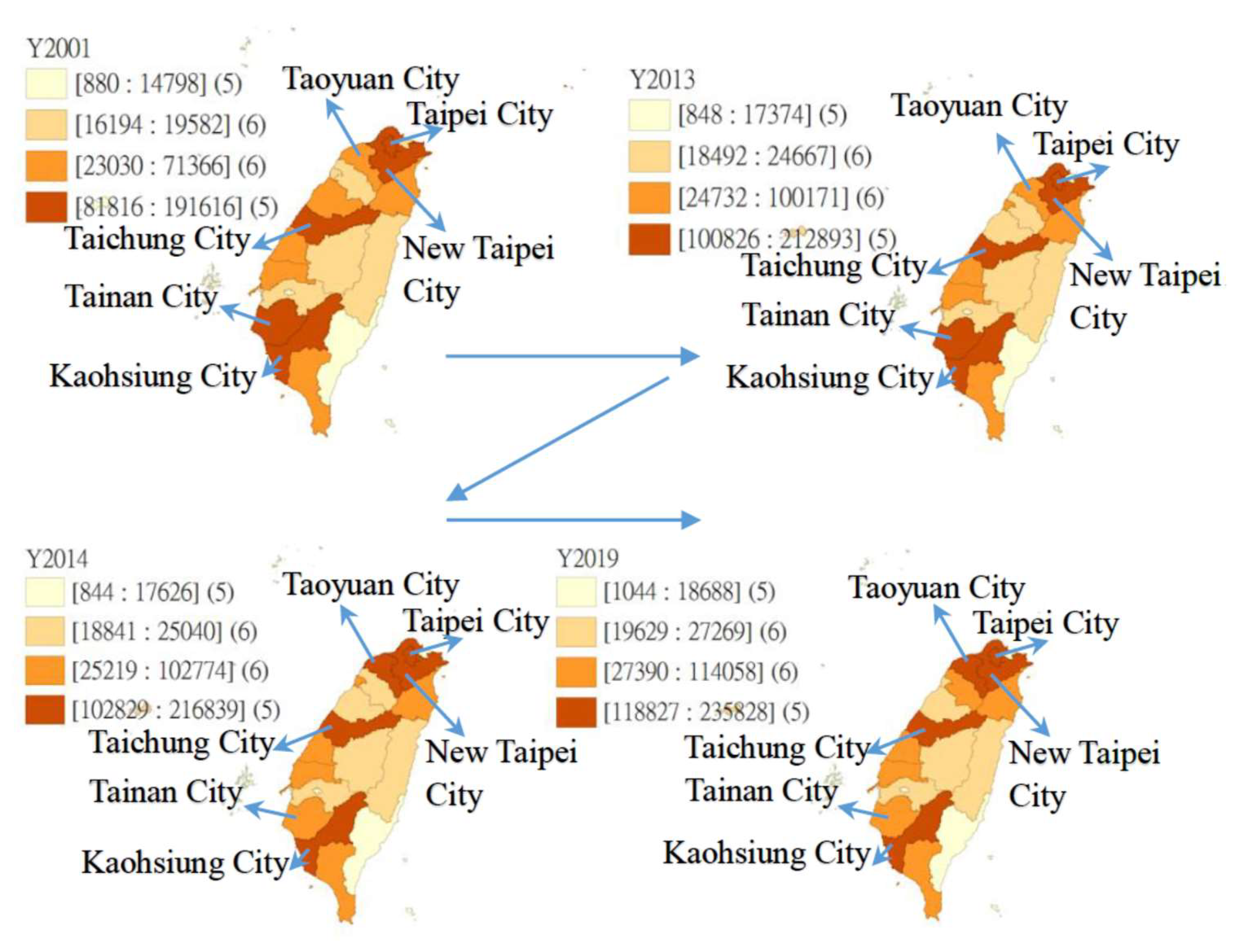
In this study, GeoDa, the spatial statistics software, was used to map the spatial distribution of the number of profit-seeking enterprises. Figure 2 shows the distribution of the number of profit-seeking enterprises in Taiwan’s counties and cities from 2001 to 2019. The darker the color, the higher the number of profit-seeking enterprises. The five municipalities, Taipei City, New Taipei City, Taichung City, Tainan City, and Kaohsiung City, maintained the highest number of profit-seeking enterprises at Level 1 from 2001 to 2013. From 2014, Taipei City, New Taipei City, Taoyuan City, Taichung City, and Kaohsiung City maintained the highest number of profit-seeking enterprises, among which Tainan City fell to Level 2 after 2014. In 2014, Taoyuan City was newly established as a municipality directly under the central government. The number of its profit-seeking enterprises rose to the first level, which shows the devotion and investment of Taoyuan City in investment promotion.
In terms of the distribution of profit-seeking enterprises in Taiwan, after Taoyuan City was upgraded to a municipality directly under the central government, the overall funds allocated by the central government to the local government and the tax revenue increased, resulting in an increase in the local fiscal expenditure budget. As a result, many profit-seeking enterprises have chosen to invest in Taoyuan City, as in Tiebout’s “vote by feet” model, where residents can choose a residential community based on their preference for public goods. During the same period, the number of profit-seeking enterprises in Tainan City continued to increase, but the increase in the number of profit-seeking enterprises in Taoyuan City was higher than that of Tainan City. This study suggests that the reason is not that the government of Tainan City performed inferiorly to Taoyuan City, but that Taoyuan City’s growth in attracting investment exceeds Tainan City.
4.3. Selection of the Spatial Econometric Model
Table 5 shows the results of the analysis and the comparison of three SAR models. The Hausman test, proposed by Hausman (1978), can be adopted to determine whether it is suitable to use the model of random effects or the model of fixed effects. Model 1 is the SAR with spatial fixed effects, Model 2 is the SAR with spatial and time fixed effects, and Model 3 is the SAR with random effects. Between Model 1 and Model 3, the Hausman test indicates x2 = 6.61, p > 0.05. The results of the Hausman test show that the null hypothesis (random effects model) is not rejected. Therefore, Model 3 is more suitable for analysis than Model 1. Between Model 2 and Model 3, the Hausman test indicates x2 = 483.42, p < 0.001. The results of the Hausman test show that the null hypothesis (random effects model) is rejected. Therefore, Model 2 is more suitable for analysis than Model 3.
Table 6 shows the results of the analysis and the comparison of the three SEM models. Model 4 is the SEM with spatial fixed effects, Model 5 is the SEN with spatial and time fixed effects, and Model 6 is SEM with random effects. Between Model 4 and Model 6, the Hausman test indicates x2 = 4.62, p > 0.05. The results of the Hausman test show that the null hypothesis (random effects model) is not rejected. Therefore, Model 6 is more suitable for analysis than Model 4. Between Model 5 and Model 6, the Hausman test indicates x2 = 379.02, p < 0.001. The results of the Hausman test show that the null hypothesis (random effects model) is rejected. Therefore, Model 5 is more suitable for analysis than Model 6.
As shown in the Hausman test results of the SAR and SEM models, the model with spatial and time fixed effects is more suitable for analysis. LeSage and Pace (2009) and Elhorst (2010, 2001) argue that the SDM can be simplified to the SAR or SEM. The model is thus selected by verifying the following hypotheses. H0: θ = 0, if the original hypothesis is rejected, then the SDM cannot be simplified to the SAR, and so it is more rational to select the SDM. H0: θ + ρβ = 0, if the original hypothesis is rejected, then the SDM cannot be simplified to the SEM, and so it is more rational to select the SDM. In Table 5, between the SAR with spatial fixed effects and the SDM with spatial fixed effects, the Wald test shows x2 = 179.78, p < 0.001, the likelihood-ratio test shows x2 = 146.18, p < 0.001, and so it is more rational to select the SDM with spatial fixed effects. Between the SAR with spatial and time fixed effects and the SDM with spatial and time fixed effects, the Wald test indicates x2 = 132.24, p < 0.001, the likelihood-ratio test indicates x2 = 128.14, p < 0.001, and so it is more reasonable to select the SDM with spatial and time fixed effects. Between the SAR with random effects and the SDM with random effects, the Wald test shows x2 = 159.79, p < 0.001, the likelihood-ratio test shows x2 = 131.78, p < 0.001, and so it is more rational to select SDM with random effects.
In Table 6, between the SEM with spatial fixed effects and the SDM with spatial fixed effects, the Wald test indicates x2 = 132.09, p < 0.001, the likelihood-ratio test indicates x2 = 128.19, p < 0.001, and so it is more reasonable to choose the SDM with spatial fixed effects. Between the SEM with spatial and time fixed effects and the SDM with spatial and time fixed effects, the Wald test shows x2 = 112.36, p < 0.001, the likelihood-ratio test shows x2 = 130.78, p < 0.001, and so it is more rational to select the SDM with spatial and time fixed effects. Between the SEM with random effects and the SDM with random effects, the Wald test shows x2 = 114.74, p < 0.001, the likelihood-ratio test shows x2 = 117.42, p < 0.001, and so it is more reasonable to choose the SDM with random effects.
The analysis results of the Wald test and likelihood-ratio test between the three models of SAR, SEM, and SDM show that the SDM is the most suitable for the analysis. As for which model of the SDMs is more suitable, we will analyze that in the next section.
4.4. Estimation Results of Various SDMs
Table 7 shows the comparison results of the SDM with spatial fixed effects and the SDM with random effects. Akaike (1973) proposed the Akaike Information Criterion (AIC) based on the Kullback–Leibler driver. Since the model with a minimum MSE (mean squared error) is selected as the adaptive model, it is more effective and sensitive. The method of AIC is to find the model that best interprets the data and contains the least free parameters. The smaller the estimated value is, the higher the goodness of fit is. Schwarz (1978) proposed the Schwartz Bayesian Information Criterion (SBC or BIC), whose lag length, corresponding to the minimum value, is the optimal lag length. This method is used to select an optimal lag term that can minimize the final prediction error. With a large number of observations, the number of parameters obtained by the BIC is less than that by the AIC. As with the AIC, when it is used for model selection, the smaller the value, the higher the model fit. The BIC is a consistent model selection method. When the sample size is large enough, the BIC selects the smallest correct model.
As far as the overall goodness of fit is concerned, the spatial econometric model uses the maximum likelihood estimation (MLE), so the maximum similar and nonlinear verification value can be obtained in the model and its coefficient can be maximized. Only the fitness test of Log-likelihood (LIK), AIC, and BIC based on the nonlinear principle can be used as the indicator of the goodness of fit. The model with the largest LIK value or the smallest AIC value and BIC value is the best model. When the AIC and BIC values are used to evaluate the goodness of fit of the model, the smaller the value, the higher the goodness of fit of the model.
Between Model 7 and Model 9, the Hausman test indicates x2 = 0.28, p > 0.05. The results of the Hausman test show that the null hypothesis (random effects model) is not rejected. Therefore, Model 9 is more suitable for analysis than Model 7. Between Model 8 and Model 9, the Hausman test indicates x2 = 39.67, p < 0.001. The results of the Hausman test show that the null hypothesis (random effects model) is rejected. Therefore, Model 8 is more suitable for analysis than Model 9. In addition, in terms of the values of Log-likelihood (LIK), AIC, and BIC for Model 8, the AIC and BIC values of Model 8 are both lower than those of Model 7 and Model 9, and the Log-likelihood (LIK) value of Model 8 is higher than that of both Model 7 and Model 9. Thus, the model fit index of Model 8 is better than that of Model 7 and Model 9. The spatial lag coefficient of Model 8 reaches a significant level (ρ = 0.182, p < 0.05), indicating significant spatial autocorrelation of the distribution in the number of profit-seeking enterprises in counties and cities, and confirming once again the rationality of incorporating the spatial effects into the econometric model. Therefore, the SDM with spatial and time fixed effects is finally selected by this study as the basis for analysis.
LeSage and Pace (2009) pointed out that in the SDM, considering the spatial interaction effects, if the regression results of the spatial estimation parameters were directly used to judge whether there is a spatial spillover effect, the feedback effects (FE) may lead to incorrect conclusions. Since the independent variables and dependent variables with spatial lag are included in the model, the estimated results cannot directly reflect their marginal effect, and it is also difficult to accurately measure the direct impact of independent variables on dependent variables (Elhorst 2010).
4.5. Decomposition Results of Direct Effects and Spillover Effects Based on SDM with Random Effects
LeSage and Pace (2009) pointed out that due to the spatial correlation between variables, it is necessary to decompose the influence of independent variables on dependent variables. They suggested that the results obtained by testing spatial spillover effects using point estimation were biased. Therefore, they proposed a partial differentiation method of the spatial regression model, which decomposes the total effect (TE) into the direct effect (DE) and indirect effect (IE). This method can better capture and explain the marginal effect of independent variables in the presence of spatial interaction. The direct effect refers to the influence of independent variables on dependent variables in the region, and the direct effects include initial effects and feedback effects. Initial effects indicate that the change to the independent variable causes the change to the dependent variable in this region. Feedback effects indicate that the change to the independent variables in this region causes the change to the dependent variables in neighboring regions, which in turn causes the change to the dependent variables in this region. In terms of numerical values, the direct effect is equal to the sum of the β regression coefficient and the feedback effect of the SDM. The indirect effect, also known as the spatial spillover effect, is used to measure the influence of an independent variable in a neighboring region on the dependent variable of the region. The total effect is equal to the sum of the direct effect and the indirect effect; that is, TE = DE + IE. It can be interpreted as the average effect of the change to an independent variable in this region on the dependent variable in all regions. Table 8 shows the results of the SDM decomposition based on fixed effects.
The following is an analysis of the spatial effects of economic development expenditure. (1) Direct effects: The growth of economic development expenditure will drive the growth in the number of profit-seeking enterprises in the region. For every 1% increase in economic development expenditure, the number of profit-seeking enterprises in the region increases by 0.083%. (2) Indirect effects: The growth of economic development expenditure has no significant effect on the number of profit-seeking enterprises in the neighboring regions. (3) Total effects: The accumulation of direct and indirect effects of economic development expenditure has no significant effect on the average number of profit-seeking enterprises in all counties and cities in Taiwan.
The following is an analysis of the spatial effect of education, science, and culture expenditure. (1) Direct effects: The growth of education, science, and culture expenditure will drive the growth in the number of profit-seeking enterprises in this region. For every 1% increase in expenditure on education, science, and culture, the number of profit-seeking enterprises in the region increased by 0.174%. (2) Indirect effects: The growth of education, science, and culture expenditure has a positive spatial spillover effect on the number of profit-seeking enterprises in neighboring regions. For every 1% increase in expenditure on education, science, and culture in neighboring regions, the number of profit-seeking enterprises in the region increases by 0.529%. The increase in expenditure on education, science, and culture in the neighboring regions has a positive effect on the number of profit-seeking enterprises in the region. (3) Total effects: The accumulation of direct and indirect effects of education, science, and culture expenditure has a positive effect on the average number of profit-seeking enterprises in all counties and cities in Taiwan. Changes in expenditure on education, science, and culture increase the total effect of the number of profit-seeking enterprises by 0.704%.
The following is an analysis of the spatial effect of the number of lighting users. (1) Direct effects: An increase in the number of lighting users prompts an increase in the number of profit-seeking enterprises in this region. Each 1% increase in the number of lighting users adds 0.086% to the number of profit-seeking enterprises in this region. (2) Indirect effects: An increase in the number of lighting users has a negative spillover effect on the number of profit-seeking enterprises in adjacent regions. Each 1% increase in the number of lighting users in the adjacent region reduces the number of profit-seeking enterprises by 0.058% in this region. (3) Total effects: The combination of the direct and indirect effects from the number of lighting users creates positive effects on the average number of profit-seeking enterprises in the cities and counties of Taiwan. The change in the number of lighting users has total effect of increasing the number of profit-seeking enterprises by 0.028%.
The following is an analysis of the spatial effect of the proportion of employees with a junior college or higher education. (1) Direct effects: An increase in the proportion of employees with a junior college or higher education prompts growth in the number of profit-seeking enterprises in this region. Each 1% increase in the proportion of employees with a junior college or higher education corresponds to a 255.002% increase in the number of profit-seeking enterprises in this region. (2) Indirect effects: An increase in the proportion of employees with a junior college or higher education has no spatial diffusion effect on adjacent regions. (3) Total effects: The aggregation of the direct and indirect effects from the proportion of employees with a junior college or higher education creates a positive impact on the average number of profit-seeking enterprises in the cities and counties of Taiwan. The change in the proportion of employees with a junior college or higher education spurs the total effect by increasing the number of profit-seeking enterprises by 475.976%.
The following is an analysis of the spatial effect of the percentage of employees aged from 25 to 44. (1) Direct effects: An increase in the percentage of employees aged between 25 and 44 prompts growth in the number of profit-seeking enterprises in this region. Each 1% increase in the percentage of employees aged from 25 to 44 leads to a 197.346% increase in the number of profit-seeking enterprises in this region. (2) Indirect effects: An increase in the percentage of employees aged between 25 and 44 has no spatial diffusion effect on adjacent regions. (3) Total effects: The combination of the direct and indirect effects of the percentage of employees aged from 25 to 44 shows a positive influence on the average number of profit-seeking enterprises in the cities and counties of Taiwan. The change in the percentage of employees aged between 25 and 44 exhibits a total effect of a 513.927% increase in the number of profit-seeking enterprises.
In terms of model selection, this study analyzed the SAR, SEM and SDM. After various tests, the SDM with spatial and time fixed effects was selected as the basis for the analysis, and the estimated results were decomposed into direct effects, indirect effects, and total effects. First, the increase in general government expenditure, economic development expenditure, expenditure on education, science, and culture, the net amount of tax collected, the number of electric lamp users, the proportion of employees with a junior college or higher education, and the percentage of employees aged 25 to 44 will increase the number of local profit-seeking enterprises, which has a positive direct effect on the number of local profit-seeking enterprises. Second, as far as the spatial dependence of the number of profit-seeking enterprises is concerned, the number of profit-seeking enterprises in different spatial locations is affected by the neighborhood effect. The increase in general government expenditure, expenditure on education, science, and culture, and the net amount of tax collected continues to spread to the neighboring regions, thus bringing the positive spatial spillover effect on the number of profit-seeking enterprises in neighboring regions. Third, the fiscal expenditure and environmental regulations with positive total effects on the average number of profit-seeking enterprises in Taiwan’s counties and cities are the general government expenditure, the expenditure on education, science, and culture, the net amount of tax collected, the number of electric lamp users, the proportion of employees with a junior college or higher education, and the percentage of employees aged 25 to 44.
4.6. Competitive Strategy of Environmental Regulation
In this study, the SDM was used to explore the impact of fiscal expenditure and environmental regulation on the number of profit-seeking enterprises in various local counties and cities, and the competitive strategies of environmental regulation adopted by local governments can be further explored. On the basis of the SDM with random effects, different types of environmental regulation competitive strategies were identified by the parameters and the direction of signs (see Table 9).
In the table, > 0 indicates that the intensity of environmental regulation is positively correlated with the number of profit-seeking enterprises in the region. In terms of the expenditure on community development and environmental protection and the ratio of the age range of employees from 25 to 44 years old, local governments adopt yardstick competition strategies for environmental regulation ( > 0, > 0). Local strengthening of environmental regulations, such as increasing the expenditure on community development and environmental protection or increasing the age range (25 to 44 years old) of employees, will lead to the same strengthening of environmental regulations in neighboring regions, which promotes the increase in the number of profit-seeking enterprises in neighboring regions, indicating that there is a positive spatial spillover effect of environmental regulation.
5. Conclusions
5.1. Conclusions and Policy Implications
Past spatial econometric models seldomly discussed Taiwan’s fiscal expenditures, labor and environmental regulations, and the economic development of profit-seeking enterprises. First, from the Moran’s I analysis on the number of profit-seeking enterprises in Taiwan, this study finds that the distribution of the number of profit-seeking enterprises in Taiwan’s counties and cities has become less and less spatially clustered in the past 19 years. This means that the spatial pattern of the distributions of profit-seeking enterprises has gradually shown a trend toward random distribution and away from clustering. It can be inferred from this phenomenon that the increase in fiscal expenditures of local governments and the improvement of labor and environmental regulations are the main reasons that have contributed to the rapid growth in the number of business operators of various counties and cities. Large numbers of profit-seeking business operators have not excessively concentrated in certain counties and cities. Therefore, Taiwan has gradually developed into an area with multiple core zones of urban development.
The preference of the government to the allocation of financial resources can be shown by the structure of fiscal expenditure, which also reflects the functions and roles of the government in the economic society. Fiscal expenditure directly supports the development of profit-seeking enterprise-related industries. The investment of local fiscal expenditure in infrastructure and other aspects will attract the investment of profit-seeking enterprises and the inflow of talents, thereby creating a spatial spillover effect on neighboring regions. Investment by local governments in economic development and education, science, and culture can promote the growth in the number of profit-seeking enterprises in the region, and the investment in economic development can also promote the growth in the number of profit-seeking enterprises in neighboring regions through the cross-border dissemination of population movement and business contacts. In other words, fiscal expenditure is an effective means of supporting the development of profit-making undertakings in various counties and cities.
As far as labor and environmental regulation is concerned, the youth group of 25 to 44 years old and the educated intellectuals with a junior college degree or above are a major driving force to invigorate the economy. Fiscal expenditure creates and lays the external developmental environment and foundation for profit-seeking enterprises, promotes the accumulation of human capital, and promotes the growth in the number of profit-seeking enterprises. Local governments should introduce policies to attract young people and intellectuals in order to increase the labor participation rate and invigorate the local market economy.
5.2. Limitations and Future Directions
This study is limited to the sample of a few independent variables where multicollinearity exists. Variable transformation was applied in the analysis, but the results were not satisfying. This study has noted that fiscal expenditures among the 22 cities and counties in Taiwan are inherently highly correlated. Furthermore, cities are divided into six municipalities and 16 non-municipalities based on the provisions of the Local Government Act of Taiwan. Taiwan’s economic development shows regional imbalance, since most of the resources and appropriations are allotted to the municipalities. The number of residents in these municipalities account for 69.45% of the total population of Taiwan. Although the fiscal expenditures of municipalities are highly correlated, dropping variables or using other variables as proxies for fiscal expenditures may influence the estimated effect of other variables on the variable of interest’s coefficient and lower the economic implications. The analysis is still based on the original fiscal expenditure variables that included samples for the period 2001 to 2019, and we ran a spatial regression with the original model specification. The results of this study thus call for future research to focus on looking at other empirical approaches for better estimates. Second, there may exist other environmental regulations that affect the growth of profit-seeking enterprises. Future researchers may consider incorporating different environmental regulatory factors into the model to investigate different environmental regulatory effects on profit-seeking enterprise numbers. Third, this study is limited to analyzing and comparing three models: the spatial autoregressive model (SAR), the spatial error model (SEM), and the spatial Durbin model (SDM). However, when spatial difference and spatial dependence coexist, traditional econometric methods are no longer applicable. Future studies may employ other analyses using different models, such as spatial dependence and spatial heterogeneity models, to explore whether the issue of spatial heterogeneity exist.
Author Contributions
Conceptualization, H.-C.H. and H.-H.L.; methodology, H.-C.H.; software, T.-H.L.; validation, T.-H.L. and H.-H.L.; formal analysis, H.-C.H. and T.-H.L.; investigation, H.-C.H. and C.-L.P.; resources, T.-H.L.; data curation, H.-C.H. and T.-H.L.; writing—original draft preparation, H.-C.H. and H.-H.L.; writing—review and editing, H.-C.H. and C.-L.P.; visualization, C.-L.P.; supervision, H.-C.H. and C.-L.P.; project administration, C.-L.P.; funding acquisition, H.-H.L. All authors have read and agreed to the published version of the manuscript.
Funding
This research received no external funding.
Institutional Review Board Statement
Not applicable.
Informed Consent Statement
Not applicable.
Data Availability Statement
Not applicable.
Conflicts of Interest
The authors declare no conflict of interest.
References
- Akaike, Hirotogu. 1973. Information theory and an extension of the maximum likelihood principle. In 2nd International Symposium on Information Theory. Edited by Boris Nikolaevic Petrov and Frigyes Csáki. Budapest: Akademiai Kiado, pp. 199–213. [Google Scholar] [CrossRef]
- Anselin, Luc. 1988. Spatial Econometrics: Methods and Models. Dordrecht: Kluwer Academic. [Google Scholar] [CrossRef] [Green Version]
- Anselin, Luc. 2003. Spatial Econometrics. In A Companion to Theoretical Econometrics. Edited by Badi Hani Baltagi. New York: Wiley, pp. 310–30. [Google Scholar] [CrossRef]
- Arrow, Kenneth J., and Mordecai Kurz. 2011. Public Investment, the Rate of Return, and Optimal Fiscal Policy. Baltimore: Johns Hopkins University Press. [Google Scholar] [CrossRef]
- Barro, Robert J. 1990. Government spending in a simple model of endogenous growth. Journal of Political Economy 98: S103–S25. [Google Scholar] [CrossRef] [Green Version]
- Bernat, George Andrew. 1996. Does manufacturing matter? A spatial econometric view of Kaldor’s laws. Journal of Regional Science 36: 463–77. [Google Scholar] [CrossRef]
- Boarnet, Marlon G. 1998. Spillovers and the locational effects of public infrastructure. Journal of Regional Science 38: 381–400. [Google Scholar] [CrossRef]
- Carruthers, John I., and Gudmundur F. Úlfarsson. 2008. Does ‘smart growth’ matter to public finance? Urban Studies 45: 1791–823. [Google Scholar] [CrossRef] [Green Version]
- Cheng, Xiao, and Yanping Pu. 2017. Effective tax rates, spatial spillover, and economic growth in China: An empirical study based on the spatial Durbin model. Annals of Economics and Finance 18: 73–97. Available online: https://ideas.repec.org/a/cuf/journl/y2017v18i1cheng.html (accessed on 26 October 2020).
- Cliff, Andrew, and Keith Ord. 1973. Spatial Autocorrelation. London: Pion. [Google Scholar] [CrossRef]
- Cliff, Andrew, and Keith Ord. 1981. Spatial Processes-Models and Applications. London: Pion. [Google Scholar]
- Cohen, Jeffrey P., and Catherine J. Morrison Paul. 2004. Public infrastructure investment, interstate spatial spillovers, and manufacturing costs. Review of Economic and Statistics 86: 551–60. Available online: http://www.jstor.org/stable/3211646 (accessed on 13 January 2020). [CrossRef]
- De Siano, Rita, and Marcella D’Uva. 2017. Fiscal decentralization and spillover effects of local government public spending: The case of Italy. Regional Studies 51: 1507–17. [Google Scholar] [CrossRef]
- Easterly, William, and Sergio Rebelo. 1993. Fiscal policy and economic growth: An empirical investigation. Journal of Monetary Economics 32: 417–58. [Google Scholar] [CrossRef]
- Elhorst, J. Paul. 2001. Dynamic models in space and time. Geographical Analysis 33: 119–40. [Google Scholar] [CrossRef] [Green Version]
- Elhorst, J. Paul. 2010. Applied spatial econometrics: Raising the bar. Spatial Economic Analysis 5: 9–28. [Google Scholar] [CrossRef]
- Fingleton, Bernard, Danilo Camargo Igliori, and Barry Moore. 2004. Employment growth of small high-technology firms and the role of horizontal clustering: Evidence from computing services and R&D in Great Britain, 1991–2000. Urban Studies 41: 773–99. [Google Scholar] [CrossRef]
- Goodchild, Michael F. 1987. A spatial analytical perspective on geographic information system. International Journal of Geographical Information System 1: 327–34. [Google Scholar] [CrossRef]
- Goodchild, Michael F., Luc Anselin, Richard P. Appelbaum, and Barbara Herr Harthorn. 2000. Toward spatially integrated social science. International Regional Science Review 23: 139–59. [Google Scholar] [CrossRef]
- Hausman, Jerry Allen. 1978. Specification tests in econometrics. Econometrica 46: 1251–71. [Google Scholar] [CrossRef] [Green Version]
- He, Ming, Yang Chen, and Ron Schramm. 2018. Technological spillovers in space and firm productivity: Evidence from China’s electric apparatus industry. Urban Studies 55: 2522–41. [Google Scholar] [CrossRef]
- Helms, Loyd Jay. 1985. The effect of state and local taxes on economic growth: A time series cross section approach. The Review of Economics and Statistics 67: 574–82. [Google Scholar] [CrossRef]
- Jiang, Lei, Haifeng Zhou, and Shixiong He. 2020. The role of governments in mitigating SO2 pollution in China: A perspective of fiscal expenditure. Environmental Science and Pollution Research 27: 33951–64. [Google Scholar] [CrossRef]
- LeSage, James, and Robbet Kelly Pace. 2009. Introduction to Spatial Econometrics. New York: CRC Press, Taylor & Francis Group. [Google Scholar] [CrossRef] [Green Version]
- Lin, Shuanglin, and Shunfeng Song. 2002. Urban economic growth in China: Theory and evidence. Urban Studies 39: 2251–66. [Google Scholar] [CrossRef]
- Morenoff, Jeffery D., and Robert J. Sampson. 1997. Violent crime and the spatial dynamics of neighborhood transition: Chicago, 1970–1990. Social Forces 76: 31–64. [Google Scholar] [CrossRef]
- Oyun, Gerel. 2017. Interstate spillovers, fiscal decentralization, and public spending on Medicaid home- and community-based services. Public Administration Review 77: 566–78. [Google Scholar] [CrossRef]
- Pan, Xiongfeng, Mengna Li, Shucen Guo, and Chenxi Pu. 2020. Research on the competitive effect of local government’s environmental expenditure in China. Science of the Total Environment 718: 137238. [Google Scholar] [CrossRef] [PubMed]
- Pereirã, Alfredo Marvão, and Oriol Roca-Sagalés. 2003. Spillovers effects of public capital formation: Evidence from the Spanish regions. Journal of Urban Economics 53: 238–56. [Google Scholar] [CrossRef] [Green Version]
- Que, Wei, Yabin Zhang, and Shaobo Liu. 2018. The spatial spillover effect of fiscal decentralization on local public provision: Mathematical application and empirical estimation. Applied Mathematics and Computation 331: 416–29. [Google Scholar] [CrossRef]
- Rey, Sergio J., and Brett Montouri. 1999. US regional income convergence: A spatial econometric perspective. Regional Studies 33: 143–56. [Google Scholar] [CrossRef]
- Sawada, Michael. 2004. Global Spatial Autocorrelation Indices- Moran’s I, Geary’s C and the General Cross-Product Statistic. Ottawa: University of Ottawa, Available online: http://www.lpc.uottawa.ca/publications/moransi/moran.htm (accessed on 21 June 2020).
- Schwarz, Gideon. 1978. Estimating the dimension of a model. The Annals of Statistics 6: 461–64. Available online: https://www.jstor.org/stable/2958889 (accessed on 1 August 2020). [CrossRef]
- Sokal, Robert R., Neal L. Oden, and Barbara A. Thomson. 1988. Local spatial autocorrelation in a biological model. Geographical Analysis 30: 331–54. [Google Scholar] [CrossRef]
- Tiebout, Charles M. 1956. A pure theory of local expenditure. Journal of Political Economy, 913–18. Available online: https://www.jstor.org/stable/1826343 (accessed on 16 January 2021). [CrossRef]
- Tobler, Waldo Rudolph. 1970. A computer movie simulating urban growth in the Detroit region. Economic Geography 46: 234–40. [Google Scholar] [CrossRef]
- Tyrrell, Timothy J., and Robert J. Johnston. 2009. An econometric analysis of the effects of tourism growth on municipal revenues and expenditures. Tourism Economics 15: 771–83. [Google Scholar] [CrossRef]
- Walter, Stephen. 1992. The analysis of regional patterns in health data. II. The power to detect environmental effects. American Journal of Epidemiology 136: 742–59. [Google Scholar] [CrossRef]
- Wang, Keliang, Shuang He, and Fuqin Zhang. 2021. Relationship between FDI, fiscal expenditure and green total-factor productivity in China: From the perspective of spatial spillover. PLoS ONE 16: e0250798. [Google Scholar] [CrossRef] [PubMed]
- Wu, Weiwei, and Jiandong Zhu. 2021. Are there demonstration effects of fiscal expenditures on higher education in China? An empirical investigation. International Journal of Educational Development 81: 102345. [Google Scholar] [CrossRef]
- Zhang, Jie, Yinxia Qu, Yun Zhang, Xiuzhen Li, and Xiao Miao. 2019. Effects of FDI on the Efficiency of Government Expenditure on Environmental Protection Under Fiscal Decentralization: A Spatial Econometric Analysis for China. International Journal of Environmental Research and Public Health 16: 2496. [Google Scholar] [CrossRef] [PubMed] [Green Version]
Figure 1.
Graph of global Moran’s I of Taiwan’s profit-seeking enterprises from 2001 to 2019.
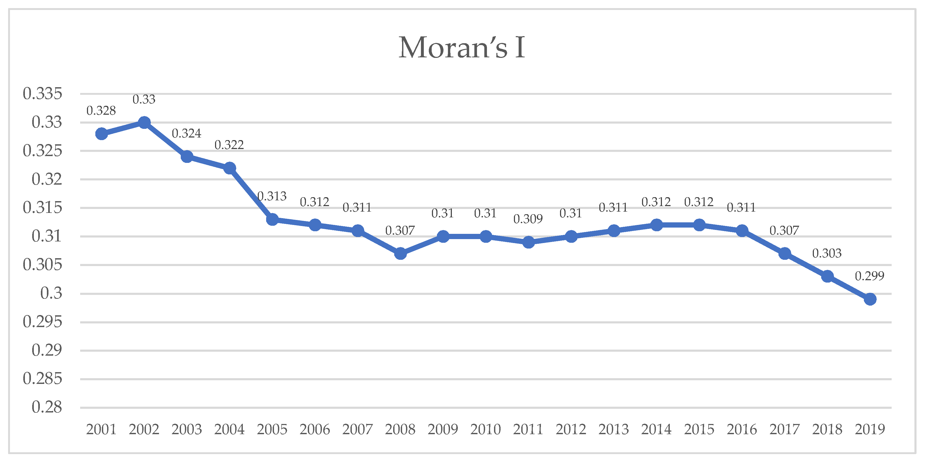
Figure 2.
Spatial distribution of Taiwan’s profit-seeking enterprises from 2001 to 2019.

Table 1.
Codes and names of 22 counties and cities in Taiwan.
| No. | Name | No. | Name | No. | Name | No. | Name |
|---|---|---|---|---|---|---|---|
| 1 | Lienchiang County | 7 | Keelung City | 13 | Taoyuan City | 18 | Kinmen County |
| 2 | Yilan County | 8 | Hsinchu City | 14 | Miaoli County | 19 | Kaohsiung City |
| 3 | Changhua County | 9 | Taipei City | 15 | Hsinchu County | 20 | Taitung County |
| 4 | Nantou County | 10 | New Taipei City | 16 | Chiayi City | 21 | Hualien County |
| 5 | Yunlin County | 11 | Taichung City | 17 | Chiayi County | 22 | Penghu County |
| 6 | Pingtung County | 12 | Tainan City |
Table 2.
Summary of descriptive statistics.
| Variables | Obs. | Mean | Std. Dev. | Min. | 25th Percentile | Median | 75th Percentile | Max. |
|---|---|---|---|---|---|---|---|---|
| NPSE | 418 | 56,699.16 | 63,026.64 | 813 | 17,353 | 24,413 | 86,319 | 235,828 |
| GGE | 418 | 4689.37 | 4995.12 | 314.69 | 1831.48 | 2417.02 | 5771.08 | 30,812.48 |
| EDE | 418 | 7194.08 | 7441.14 | 881.11 | 2596.07 | 4359.20 | 8333.14 | 47,178.08 |
| EESC | 418 | 15,098.66 | 16,282.09 | 463.52 | 4959.05 | 4959.04 | 19,860.31 | 65,587.43 |
| ECDEP | 418 | 2369.52 | 3710.74 | 88.11 | 310.10 | 683.84 | 2026.77 | 16,149.67 |
| NATC | 418 | 80,633,469.67 | 140,544,536.26 | 91,613.62 | 8,530,115 | 26,300,000 | 104,000,000 | 789,241,887.60 |
| NLU | 418 | 557,416.83 | 540,259.25 | 3635 | 174,403 | 174,403 | 174,403 | 2,058,119 |
| LFPR | 418 | 57.92 | 3.99 | 46 | 56.3 | 57.9 | 59.3 | 74.90 |
| PEE | 418 | 37.38 | 12.81 | 9.74 | 28.81 | 36.01 | 44.49 | 81.05 |
| PEA | 418 | 54.69 | 4.90 | 37.49 | 51.86 | 55.16 | 57.93 | 63.97 |
Note: NPSE: Number of profit-seeking enterprises; GGE: General government expenditure (TWD million); EDE: Economic development expenditure (TWD million); EESC: Expenditure on education, science, and culture (TWD million); ECDEP: Expenditure on community development and environmental protection (TWD million); NATC: Net amount of tax collected (TWD thousand); LFPR: Labor force participation rate (%); NLU: Number of lighting users; PEE: Proportion of employees with junior college or higher education (%); PEA: Percentage of employees aged 25 to 44 (%).
Table 3.
Pearson correlation analysis.
| NPSE | GGE | EDE | ECE | CEE | ACN | LFP | LU | ESE | AEP | |
|---|---|---|---|---|---|---|---|---|---|---|
| NPSE | 1 | |||||||||
| GGE | 0.865 *** | 1 | ||||||||
| EDE | 0.869 *** | 0.837 *** | 1 | |||||||
| EESC | 0.971 *** | 0.885 *** | 0.892 *** | 1 | ||||||
| ECDEP | 0.911 *** | 0.866 *** | 0.859 *** | 0.930 *** | 1 | |||||
| NATC | 0.794 *** | 0.690 *** | 0.738 *** | 0.855 *** | 0.815 *** | 1 | ||||
| LFPR | 0.934 *** | 0.831 *** | 0.798 *** | 0.883 *** | 0.801 *** | 0.579 *** | 1 | |||
| NLU | 0.050 | 0.066 | 0.031 | 0.043 | 0.018 | 0.005 | 0.103 * | 1 | ||
| PEE | 0.491 *** | 0.493 *** | 0.452 *** | 0.536 *** | 0.563 *** | 0.647 *** | 0.321 *** | 0.127 ** | 1 | |
| PEA | 0.225 *** | 0.072 | 0.093 | 0.177 *** | 0.157 ** | 0.144 ** | 0.236 *** | 0.094 | 0.080 | 1 |
Note: * p < 0.05, ** p < 0.01, *** p < 0.001.
Table 4.
Spatial autocorrelation statistics from 2001 to 2019.
| Year | Moran’s I | Year | Moran’s I | ||
|---|---|---|---|---|---|
| I | p-Value | I | p-Value | ||
| 2001 | 0.328 | 0.025 | 2011 | 0.309 | 0.036 |
| 2002 | 0.330 | 0.025 | 2012 | 0.310 | 0.035 |
| 2003 | 0.324 | 0.028 | 2013 | 0.311 | 0.035 |
| 2004 | 0.322 | 0.029 | 2014 | 0.312 | 0.035 |
| 2005 | 0.313 | 0.033 | 2015 | 0.312 | 0.035 |
| 2006 | 0.312 | 0.034 | 2016 | 0.311 | 0.035 |
| 2007 | 0.311 | 0.035 | 2017 | 0.307 | 0.038 |
| 2008 | 0.307 | 0.037 | 2018 | 0.303 | 0.040 |
| 2009 | 0.310 | 0.035 | 2019 | 0.299 | 0.042 |
| 2010 | 0.310 | 0.036 | |||
Table 5.
Estimation results of fixed effects and random effects of spatial autoregressive model (SAR).
Table 5.
Estimation results of fixed effects and random effects of spatial autoregressive model (SAR).
| Spatial Autoregressive Model (SAR): ~ N (0, σ2 I) is an n-dimensional vector of i,i,d disturbances following multiple normal distributions with zero mean and finite variances. | ||||||
| Variables | Model 1 SAR with Spatial Fixed Effects | Model 2 SAR with Spatial and Time Fixed Effects | Model 3 SAR with Random Effects | |||
| Coefficient | p-Value | Coefficient | p-Value | Coefficient | p-Value | |
| GGE | 0.448 *** | 0.000 | 0.558 *** | 0.000 | 0.416 *** | 0.000 |
| EDE | 0.035 | 0.365 | 0.066 | 0.060 | 0.038 | 0.334 |
| EESC | 0.148 * | 0.033 | 0.063 | 0.312 | 0.178 * | 0.012 |
| ECDEP | 0.449 ** | 0.002 | 0.415 ** | 0.001 | 0.445 ** | 0.002 |
| NATC | 0.000 *** | 0.000 | 0.000 *** | 0.000 | 0.000 *** | 0.000 |
| NLU | 0.082 *** | 0.000 | 0.085 *** | 0.000 | 0.082 *** | 0.000 |
| LFPR | 257.466 * | 0.017 | 336.785 ** | 0.001 | 256.833 * | 0.019 |
| PEE | −108.494 * | 0.019 | 501.005 *** | 0.000 | −106.946 * | 0.020 |
| PEA | 65.021 | 0.403 | 76.645 | 0.372 | 82.816 | 0.297 |
| Constant | −17,516.800 | 0.077 | ||||
| n | 418 | 418 | 418 | |||
| 0.070 * | 0.031 | 0.032 | 0.334 | 0.078 * | 0.013 | |
| within R2 | 0.913 | 0.834 | 0.912 | |||
| between R2 | 0.933 | 0.950 | 0.937 | |||
| overall R2 | 0.933 | 0.943 | 0.937 | |||
| Log-likelihood | −3848.553 | −3809.588 | −3934.340 | |||
| AIC | 7715.106 | 7637.175 | 7890.68 | |||
| BIC | 7751.425 | 7673.495 | 7935.07 | |||
| 6.61 | 483.42 | |||||
| Hausman p-value | 0.470 | 0.000 | ||||
| Wald test | = 0 = 179.78 p-value = 0.0000 | = 0 = 132.24 p-value = 0.0000 | = 0 = 159.79 p-value = 0.0000 | |||
| (1) | = 128.14 p-value = 0.0000 | = 131.78 p-value = 0.0000 | ||||
Note: * p < 0.05, ** p < 0.01, *** p < 0.001.
Table 6.
Estimation results of fixed effects and random effects of spatial error model (SEM).
| Spatial Error Model (SEM): ~ N (0, σ2 I) ; ε is an i.i.d noise. | ||||||
| Variables | Model 4 SEM with Spatial Fixed Effects | Model 5 SEM with Spatial and Time Fixed Effects | Model 6 SEM with Random Effects | |||
| Coefficient | p-Value | Coefficient | p-Value | Coefficient | p-Value | |
| GGE | 0.397 *** | 0.000 | 0.569 *** | 0.000 | 0.369 *** | 0.000 |
| EDE | 0.023 | 0.500 | 0.063 | 0.081 | 0.026 | 0.465 |
| EESC | 0.035 | 0.592 | 0.067 | 0.310 | 0.061 | 0.362 |
| ECDEP | 0.417 ** | 0.002 | 0.429 ** | 0.001 | 0.423 ** | 0.002 |
| NATC | 0.000 *** | 0.000 | 0.000 *** | 0.000 | 0.000 *** | 0.000 |
| NLU | 0.091 *** | 0.000 | 0.084 *** | 0.000 | 0.090 *** | 0.000 |
| LFPR | 177.136 | 0.098 | 387.871 *** | 0.000 | 169.164 | 0.124 |
| PEE | −9.416 | 0.863 | 544.884 *** | 0.000 | 3.033 | 0.958 |
| PEA | 82.254 | 0.320 | 64.136 | 0.477 | 98.888 | 0.242 |
| Constant | −15,627.800 | 0.111 | ||||
| n | 418 | 418 | 418 | |||
| 0.406 *** | 0.000 | 0.010 | 0.898 | 0.410 *** | 0.000 | |
| within R2 | 0.909 | 0.830 | 0.910 | |||
| between R2 | 0.922 | 0.951 | 0.926 | |||
| overall R2 | 0.922 | 0.943 | 0.926 | |||
| Log-likelihood | −3839.559 | −3810.908 | −3927.159 | |||
| AIC | 7697.118 | 7639.815 | 7876.317 | |||
| BIC | 7733.438 | 7676.135 | 7920.708 | |||
| 4.62 | 379.02 | |||||
| Hausman p-value | 0.707 | 0.000 | ||||
| Wald test | = 132.09 p-value = 0.0000 | = 0 = 112.36 p-value = 0.0000 | = 114.74 p-value = 0.0000 | |||
| Likelihood-ratio test | = 128.19 p-value = 0.0000 | = 130.78 p-value = 0.0000 | = 117.42 p-value = 0.0000 | |||
Note: ** p < 0.01, *** p < 0.001.
Table 7.
Estimation results of fixed effects and random effects of spatial Durbin model (SDM).
| Spatial Durbin Model (SDM): ~ N (0, σ2 I) is the error term of the spatial autocorrelation. | ||||||
| Variables | Model 7 SDM with Spatial Fixed Effects | Model 8 SDM with Spatial and Time Fixed Effects | Model 9 SDM with Random Effects | |||
| Coefficient | p-Value | Coefficient | p-Value | Coefficient | p-Value | |
| GGE | 0.202 * | 0.011 | 0.337 *** | 0.000 | 0.218 ** | 0.007 |
| EDE | 0.098 ** | 0.003 | 0.087 ** | 0.007 | 0.100 ** | 0.003 |
| EESC | 0.134 * | 0.027 | 0.147 * | 0.013 | 0.144 * | 0.021 |
| ECDEP | 0.256 * | 0.037 | 0.228 | 0.057 | 0.258 * | 0.042 |
| NATC | 0.000 *** | 0.000 | 0.000 *** | 0.000 | 0.000 *** | 0.000 |
| NLU | 0.093 *** | 0.000 | 0.089 *** | 0.000 | 0.092 *** | 0.000 |
| LFPR | 41.294 | 0.665 | 127.183 | 0.197 | 26.286 | 0.789 |
| PEE | 213.426 *** | 0.000 | 249.263 * | 0.017 | 233.193 *** | 0.000 |
| PEA | 139.467 | 0.060 | 178.889 * | 0.026 | 148.154 * | 0.046 |
| W×GGE | 0.266* | 0.010 | 0.625 *** | 0.000 | 0.200 | 0.061 |
| W×EDE | −0.072 | 0.157 | −0.072 | 0.169 | −0.086 | 0.095 |
| W×EESC | 0.450 *** | 0.000 | 0.482 *** | 0.000 | 0.382 *** | 0.000 |
| W×ECDEP | 0.030 | 0.841 | 0.034 | 0.825 | 0.058 | 0.710 |
| W×NATC | 0.000 ** | 0.004 | 0.000 | 0.092 | 0.000 ** | 0.003 |
| W×NLU | −0.072 *** | 0.000 | −0.072 *** | 0.000 | −0.057 *** | 0.000 |
| W×LFPR | 88.822 | 0.674 | 294.051 | 0.207 | 182.973 | 0.195 |
| W×PEE | −162.803 | 0.050 | 158.341 | 0.120 | −252.968 ** | 0.003 |
| W×PEA | −84.484 | 0.520 | 267.261 | 0.152 | −18.823 | 0.846 |
| Constant | −13019 | 0.259 | ||||
| n | 418 | 418 | 418 | |||
| 0.324 *** | 0.000 | 0.182 * | 0.046 | 0.312 *** | 0.000 | |
| within R2 | 0.934 | 0.916 | 0.934 | |||
| between R2 | 0.885 | 0.823 | 0.918 | |||
| overall R2 | 0.886 | 0.824 | 0.918 | |||
| Log-likelihood | −3775.465 | −3745.520 | −3868.450 | |||
| AIC | 7582.93 | 7523.039 | 7772.9 | |||
| BIC | 7647.498 | 7587.607 | 7845.539 | |||
| 0.28 | 39.67 | |||||
| Hausman p-value | 0.100 | 0.000 | ||||
Note: * p < 0.05, ** p < 0.01, *** p < 0.001.
Table 8.
Direct, indirect, and total effects of SDM with spatial and time fixed effects.
| Variables | LR_Direct Effect | LR_Indirect Effect | LR_Total Effect | |||
| Coefficient | p-Value | Coefficient | p-Value | Coefficient | p-Value | |
| GGE | 0.370 *** | 0.000 | 0.709 *** | 0.000 | 1.079 *** | 0.000 |
| EDE | 0.083 ** | 0.009 | −0.059 | 0.276 | 0.024 | 0.731 |
| EESC | 0.174 ** | 0.004 | 0.529 *** | 0.000 | 0.704 *** | 0.000 |
| ECDEP | 0.225 | 0.052 | 0.064 | 0.683 | 0.289 | 0.194 |
| NATC | 0.000 *** | 0.000 | 0.000 * | 0.012 | 0.000 *** | 0.000 |
| NLU | 0.086 *** | 0.000 | −0.058 *** | 0.000 | 0.028 * | 0.021 |
| LFPR | 142.947 | 0.177 | 323.182 | 0.199 | 466.129 | 0.123 |
| PEE | 255.002 * | 0.014 | 220.974 | 0.068 | 475.976 ** | 0.004 |
| PEA | 197.346 * | 0.014 | 316.581 | 0.108 | 513.927 * | 0.020 |
Note: LR_Direct Effect = Coefficient of SDM + feedback effect; LR_Indirect Effect = Spatial spillover effect; LR_Total Effect = Direct effect + indirect effect. * p < 0.05, ** p < 0.01, *** p < 0.001.
Table 9.
Competitive strategy of environmental regulation.
| Coefficient | > 0 | < 0 |
| > 0 | The stronger the environmental regulation, the higher the number of local profit-seeking enterprises, and local governments adopt the strategy of yardstick competition in environmental regulation. The yardstick competition strategy shows that the interactive behavior pattern of environmental regulation between local governments is “you are strong and I am strong”. → General government expenditure → Expenditure on education, science and culture | The stronger the environmental regulation, the lower the number of local profit-seeking enterprises, and local governments adopt the strategy of differentiated competition in environmental regulation. The differentiated competition strategy shows that the interactive behavior pattern of environmental regulation among local governments is “you are strong and I am weak”. |
| < 0 | The stronger the environmental regulation, the higher the number of local profit-seeking enterprises, and local governments adopt the strategy of differentiated competition in environmental regulation. The differentiated competition strategy shows that the interactive behavior pattern of environmental regulation among local governments is “you are weak and I am strong”. → Number of lighting users | The stronger the environmental regulation, the lower the number of local profit-seeking enterprises, and local governments adopt the strategy of racing to the bottom in environmental regulation. The “race to the bottom” competition strategy indicates that the interactive behavior pattern of environmental regulation among local governments is “you are weak and I am weak”. |
Publisher’s Note: MDPI stays neutral with regard to jurisdictional claims in published maps and institutional affiliations. |
© 2022 by the authors. Licensee MDPI, Basel, Switzerland. This article is an open access article distributed under the terms and conditions of the Creative Commons Attribution (CC BY) license (https://creativecommons.org/licenses/by/4.0/).
Share and Cite
MDPI and ACS Style
Huang, H.-C.; Liu, H.-H.; Peng, C.-L.; Liao, T.-H. Do Local Fiscal Expenditures Promote the Growth of Profit-Seeking Enterprise Numbers in Neighboring Areas? Economies 2022, 10, 34. https://doi.org/10.3390/economies10020034
AMA Style
Huang H-C, Liu H-H, Peng C-L, Liao T-H. Do Local Fiscal Expenditures Promote the Growth of Profit-Seeking Enterprise Numbers in Neighboring Areas? Economies. 2022; 10(2):34. https://doi.org/10.3390/economies10020034
Chicago/Turabian StyleHuang, Hao-Chen, Hsin-Hung Liu, Chi-Lu Peng, and Ting-Hsiu Liao. 2022. "Do Local Fiscal Expenditures Promote the Growth of Profit-Seeking Enterprise Numbers in Neighboring Areas?" Economies 10, no. 2: 34. https://doi.org/10.3390/economies10020034
Note that from the first issue of 2016, this journal uses article numbers instead of page numbers. See further details here.