Characterization of Fading Statistics of mmWave (28 GHz and 38 GHz) Outdoor and Indoor Radio Propagation Channels ^†

Abstract

Extension of usable frequency spectrum from microwave to millimeter-wave (mmWave) is one of the key research directions in addressing the capacity demands of emerging 5th-generation communication networks. This paper presents a thorough analysis on the azimuthal multipath shape factors and second-order fading statistics (SOFS) of outdoor and indoor mmWave radio propagation channels. The well-established analytical relationship of plain angular statistics of a radio propagation channel with the channel’s fading statistics is used to study the channel’s fading characteristics. The plain angle-of-arrival measurement results available in the open literature for four different outdoor radio propagation scenarios at 38 GHz, as well as nine different indoor radio propagation scenarios at 28 GHz and 38 GHz bands, are extracted by using different graphical data interpretation techniques. The considered quantifiers for energy dispersion in angular domain and SOFS are true standard-deviation, angular spread, angular constriction, and direction of maximum fading; and spatial coherence distance, spatial auto-covariance, average fade duration, and level-crossing-rate; respectively. This study focuses on the angular spread analysis only in the azimuth plane. The conducted analysis on angular spread and SOFS is of high significance in designing modulation schemes, equalization schemes, antenna-beams, channel estimation, error-correction techniques, and interleaving algorithms; for mmWave outdoor and indoor radio propagation environments.

1. Introduction

In the recent years, an explosive growth in mobile communication networks has been observed, which has led to a boom of new applications and data services. This growth has emerged as a global challenge for service providers and researchers to meet the capacity demands of the emerging 5th generation (5G) of wireless communication networks. In this context, the extension and efficient-use of usable frequency spectrum is believed to be of vital importance. Expansion of usable frequency spectrum to higher bands of frequencies, i.e., millimeter-wave (mmWave), is thought to be a potential research direction to address the capacity demands.

Accurate understanding of radio propagation channel characteristics helps in devising efficient signal processing algorithms and designs for receivers to meet the capacity demands of emerging wireless communication networks. Analysis of angular spread and second-order fading statistics (SOFS) of land-mobile radio cellular communication channels is thoroughly studied in the literature, e.g., [1,2]. For different scenarios of terrestrial communications, such studies investigate the characteristics of the channel in angular, Doppler and delay domain. Several studies [3,4,5,6,7,8] have been presented in the literature to study the channel characteristics for mmWave band, mainly at 28 GHz and 38 GHz. In [3], measurements are presented which were conducted for outdoor cellular propagation environments at 28 GHz in New York City; where Path loss, angular statistics, and delay statistics are studied. In [4], channel measurements are presented for outdoor urban environment at 38 GHz. Angle-of-arrival (AoA) analysis is presented for different locations of receiver (Rx) and transmitter (Tx) with antennas of different gains. A study presented in [5], provides an analytical relationship for SOFS of mmWave communication channels. In [6], spatial and temporal characteristics of indoor radio channels for 28 GHz mmWave band are studied; particularly for an indoor office environment. Similarly, in [7], channel measurements are conducted in an indoor corridor radio propagation environment for mmWave range at 19 GHz, 28 GHz, and 38 GHz bands. Various dynamic challenges in addressing the demands of emerging 5G communication networks, demand conduction of an intensive research to study both the large- and small-scale fading statistics of both indoor and outdoor mmWave radio propagation channels.

Mobility of mobile user terminals and the spread of energy in angular domain determines Doppler spread, which further has a direct relationship with the rate of fluctuations in the received signals envelopes. These fluctuations at small and large scale in the received signal’s envelope affect the performance of error-correction algorithms, modulation schemes, equalization, diversity, and channel coding techniques. Therefore, it is imperative to have a comprehensive understanding of the dispersion of energy in angular domain, which further helps in characterization of SOFS of the channels. A theory of multipath shape factors (SFs) is proposed by Durgin et al. in [9,10] which provides a direct analytical method for quantification of the dispersion of energy along azimuth AoA. The proposed SFs are named as, angular constriction, angular spread, and direction of maximum fading. Moreover, novel analytical relationships of these SFs with SOFS of the radio propagation channels are also proposed. These SOFS quantifiers are spatial auto-covariance (ACV), coherence distance (CD), average fade duration (AFD), and level-crossing-rate (LCR). Modeling the AoA in 3D domain is of high significance. Many studies proposed in literature [11,12,13] present different methods for determining the arrival angles and their intensity. In [14,15], the characterization of angular spread in 3D scenarios is presented in terms of SFs. In [16,17], a new angular spread quantifier, named true standard deviation, is proposed; moreover, a new definition of SFs is also provided. These SFs are used to study the Nakagami-m and Nakagami-hoyt fading channels in [18,19], respectively. A SOFS-based analysis of channel simulators implementing Nakagami fading is presented in [20]. A detailed analysis on characterization of angular spread and SOFS of air-to-ground and different outdoor land-mobile radio communication channels for both empirical and geometric channel models is conducted in [21,22,23,24,25]. A study conducted in [26], presents an analysis on SOFS of mmWave communication channel in outdoor radio propagation environment at 28 GHz. No such studies, for angular-spread and SOFS quantification of outdoor mmWave (38 GHz) and indoor mmWave (28 GHz) radio propagation channels are available in the literature, to the best of authors’ knowledge. Therefore, there is a significant scope to conduct a thorough study for quantification of angular spread and characterization of fading statistics of outdoor and indoor mmWave radio propagation channels.

In this paper, the measurement results presented in [4,6,7] for plain AoA statistics of different outdoor and indoor radio propagation scenarios at 28 and 38 GHz frequency bands are extended to the quantification of dispersion of energy in azimuthal domain and characterization of SOFS of the radio channel. The conducted analysis is of high significance in designing receivers, antennas spacing, interleaving schemes, interference mitigation, modulation schemes, and error-correction codes, etc. The details of considered measurement data-sets, propagation scenarios, and the proposed work are presented in

Table 1. Characteristics of considered measurement scenarios and the proposed extensions.

Measurement Scenario	Propagation Environment	Frequency Band	Channel Statistics
			Available	Proposed Extension
Case 1 [4]	Outdoor Urban	38 GHz	Path Loss, Root Mean Square (RMS) Delay Spread, AoA	Azimuthal Spread Quantification, LCR, AFD, CD, Auto-Correlations
Case 2 [7]	Indoor Corridor	28 and 38 GHz	Path Loss, RMS Delay Spread, AoA	Azimuthal Spread Quantification, LCR, AFD, CD, Auto-Correlations
Case 3 [6]	Indoor Office	28 GHz	Delay Spread, AoA, Time of Arrival	Azimuthal Spread Quantification, LCR, AFD, CD, Auto-Correlations

. A part of this work was presented in [27] where only one indoor measurement dataset was used to analyze the azimuthal spread and SOFS of indoor radio propagation channels. However, this paper extends the work by including analysis on three more measurement data-sets for different indoor and outdoor mmWave radio propagation scenarios. A detailed analysis on the impact of variations in Doppler frequency, link-distance, and observation amplitude level on the AFD, LCR, CD, and spatial auto-covariance is conducted. This study focuses on the angular spread analysis only in the azimuth plane. The remaining of the paper is organized as follows: Measurement setup for all the cases is explained in Section 2. The detailed channel characteristics, proposed methodology and discussion on obtained results are given in Section 3. Finally, the conclusion is given in Section 4.

2. Overview of Measurement Setup and Used Data-Extraction Method

In this paper, the measurement results presented in [4,6,7], for different outdoor and indoor scenarios are extended from plain spatial characteristics of mmWave radio propagation channels to the quantification of energy in angular domain and characterization of SOFS of the radio channel.

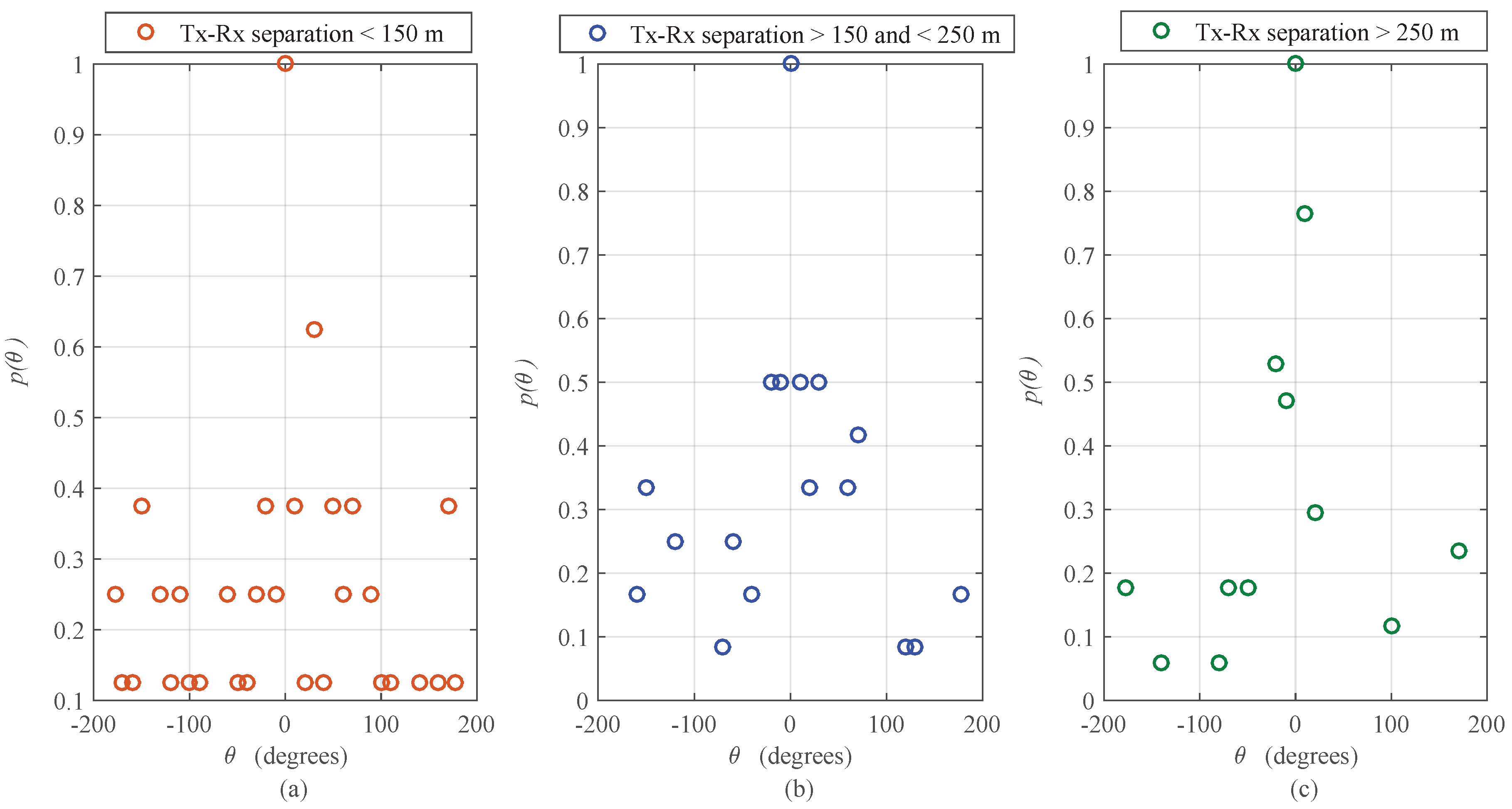
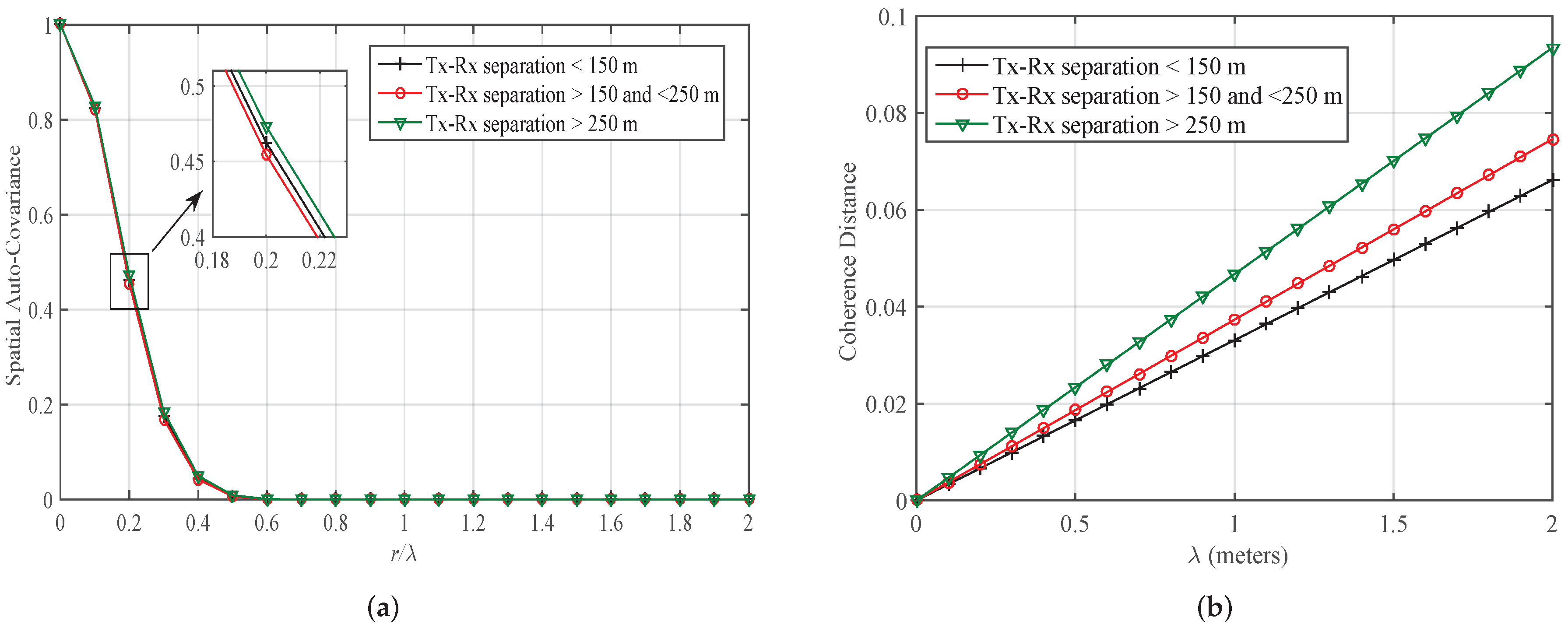
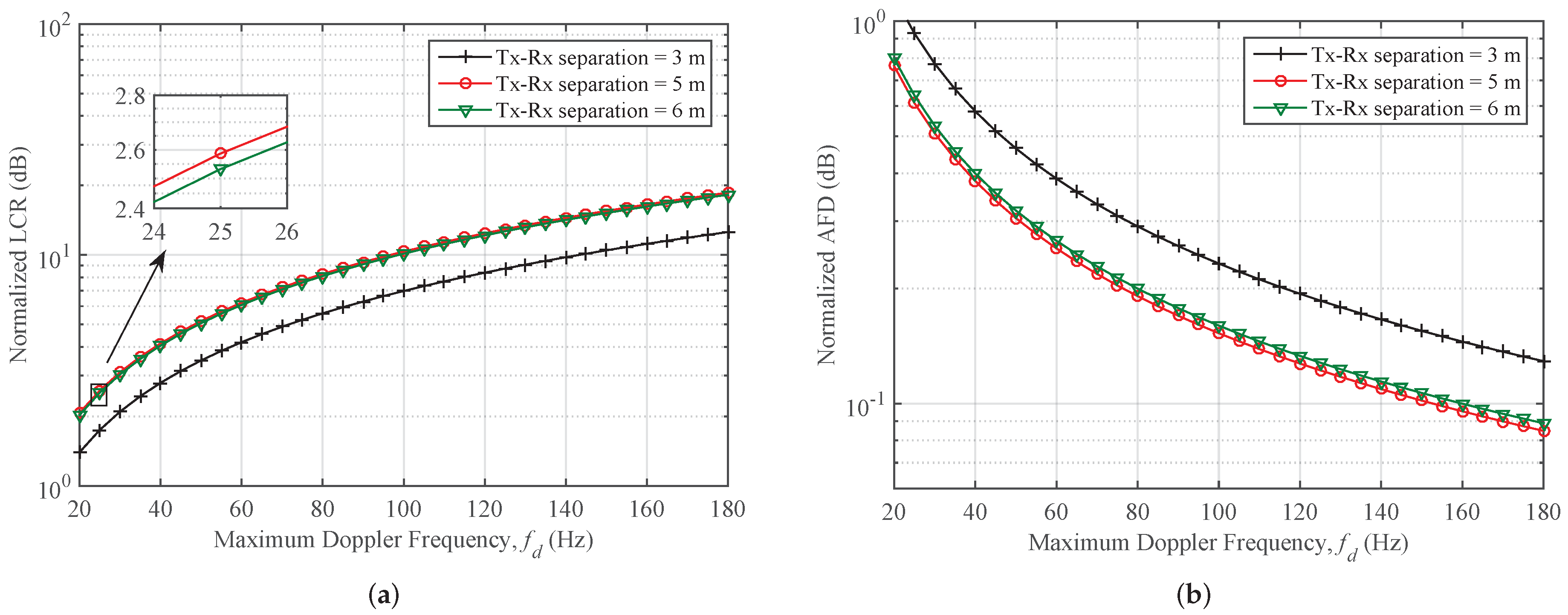
2.1. Case 1: Outdoor Urban Environment at 38 GHz

In [4], measurement campaign is conducted for measuring different channel parameters in University of Texas at Austin campus for outdoor environment. The study is conducted at mmWave (38 GHz) band. The Tx was placed at different rooftop locations within the University. The antenna to transmit is mounted on a tripod 1.5 m above the roof. At locations of Rx, measurements are obtained by using steerable antennas with a 25 dBi vertically polarized rectangular horn antenna. The separation of Rx from Tx ranges from 75 m to 295 m. Rx is placed at 11 different locations and out of these 11 five were obstructed and six locations had clear line-of-sight (LoS) using the 25 dBi antenna. In selected measurements, three different scenarios are presented. In scenario 1: the distance between Tx and Rx is less than 150 m; scenario 2 covers the cases where the distance between Tx and Rx is greater than 150 m and less than 250 m. Scenario 3 covers all the measurement locations where the distance between Tx and Rx is greater than 250 m.

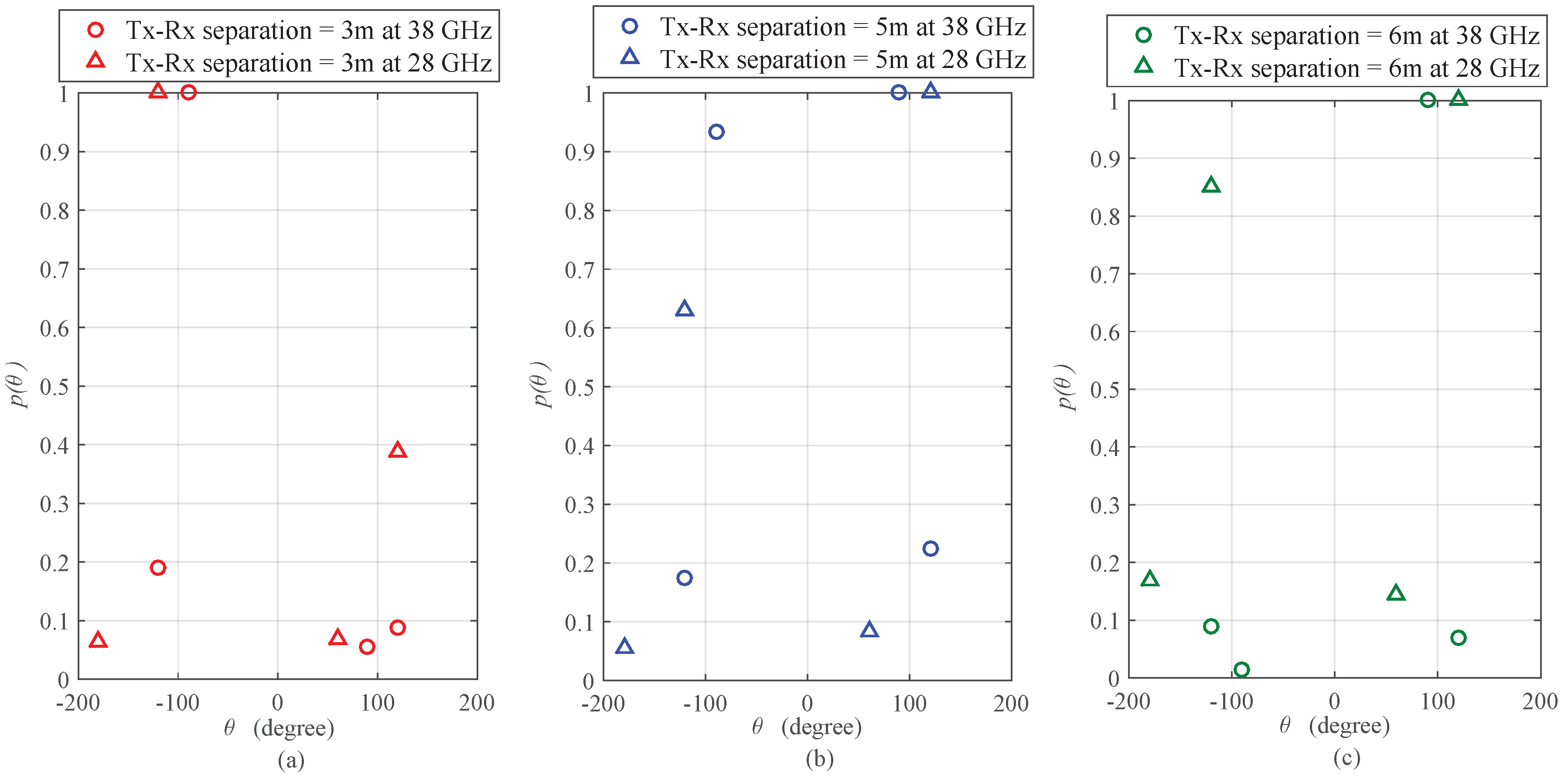
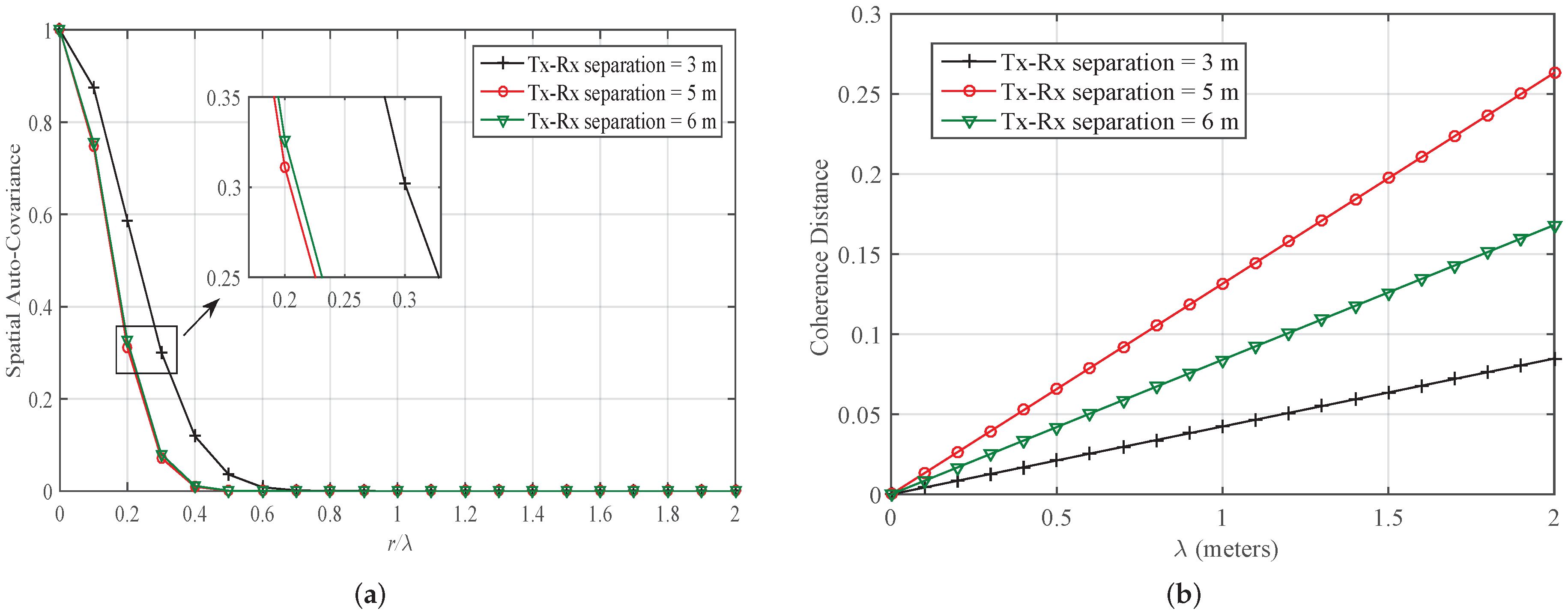
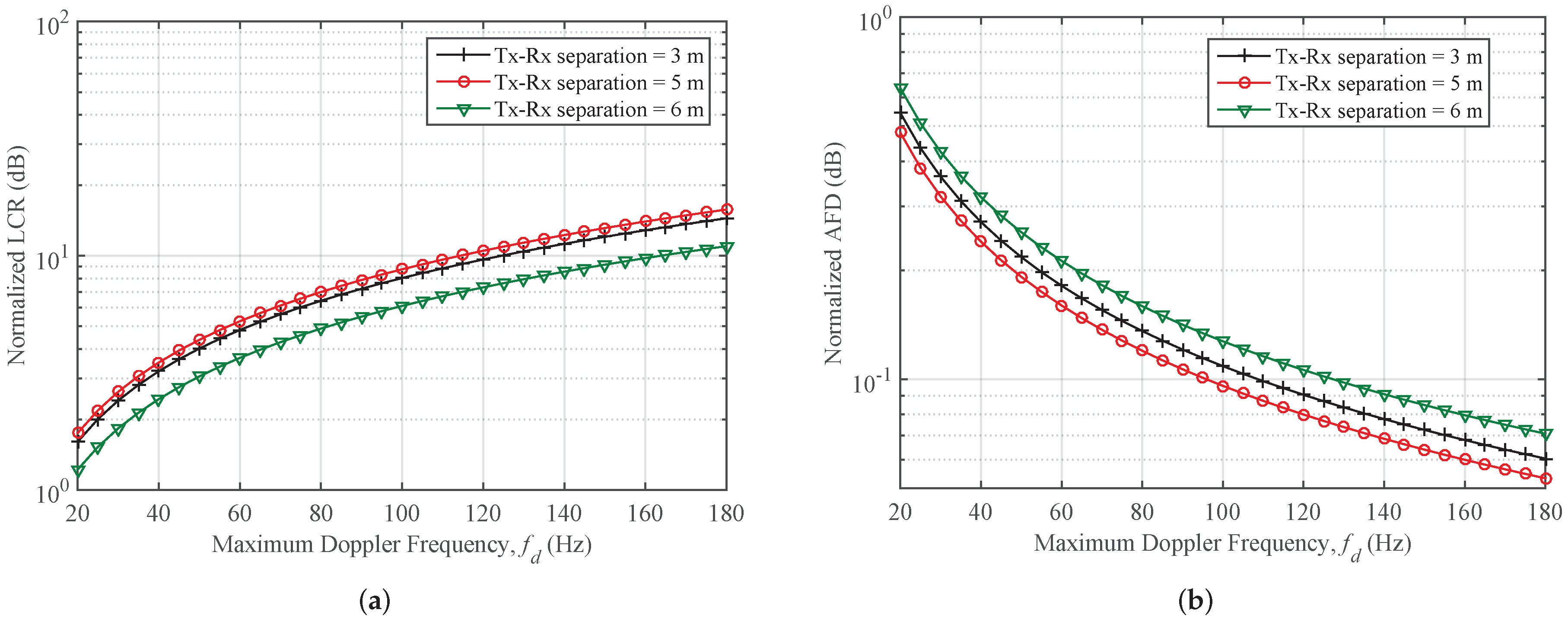
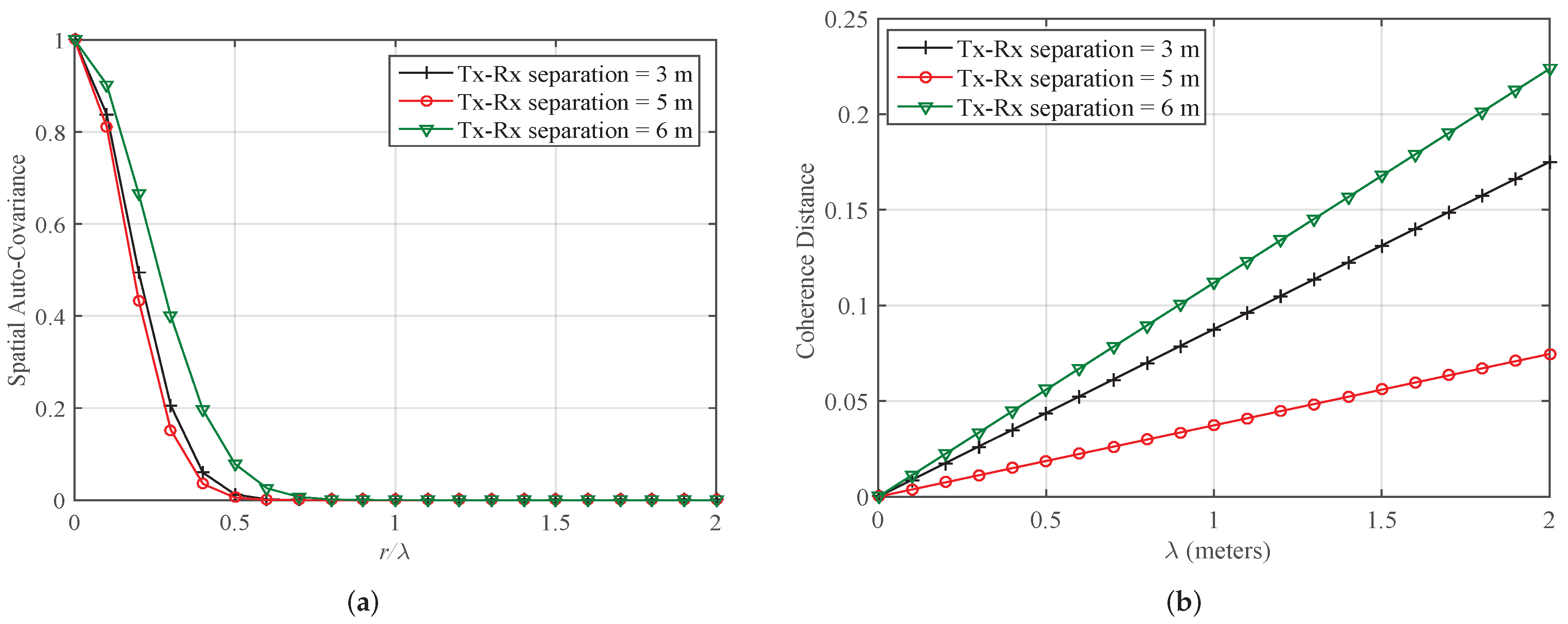
2.2. Case 2: Indoor Corridor Environment at 28 GHz and 38 GHz

In [7], a campaign is conducted for channel measurements in indoor corridor environment for mmWave frequencies at 28 GHz, and 38 GHz. The experiment is conducted in Malaysia on the second floor of the Menara Tun Razak Building of Universiti Teknologi Malaysia (UTM). The corridor size where measurements are taken is 67 m × 1.80 m. The height of roof is 3 m. The corridor has glass door, concrete walls, gypsum boards and plywood. Glazed ceramic tiles have covered the floor and the fiberglass material is used in the ceiling. While conducting measurements, Tx remained unmoved and Rx is moved along different directions. The height of Tx and Rx from the floor are 1.7 m and 1.5 m, respectively. The measurements extended here are taken for non-LoS (NLoS) scenarios. Three different scenarios are taken, and the results are recorded by changing the distance between Tx and Rx from 3 m, to 5 m, and 6 m, at 28 GHz. Same setup is repeated by changing the frequency band to 38 GHz. The results of AoA distributions are presented with respect to received power.

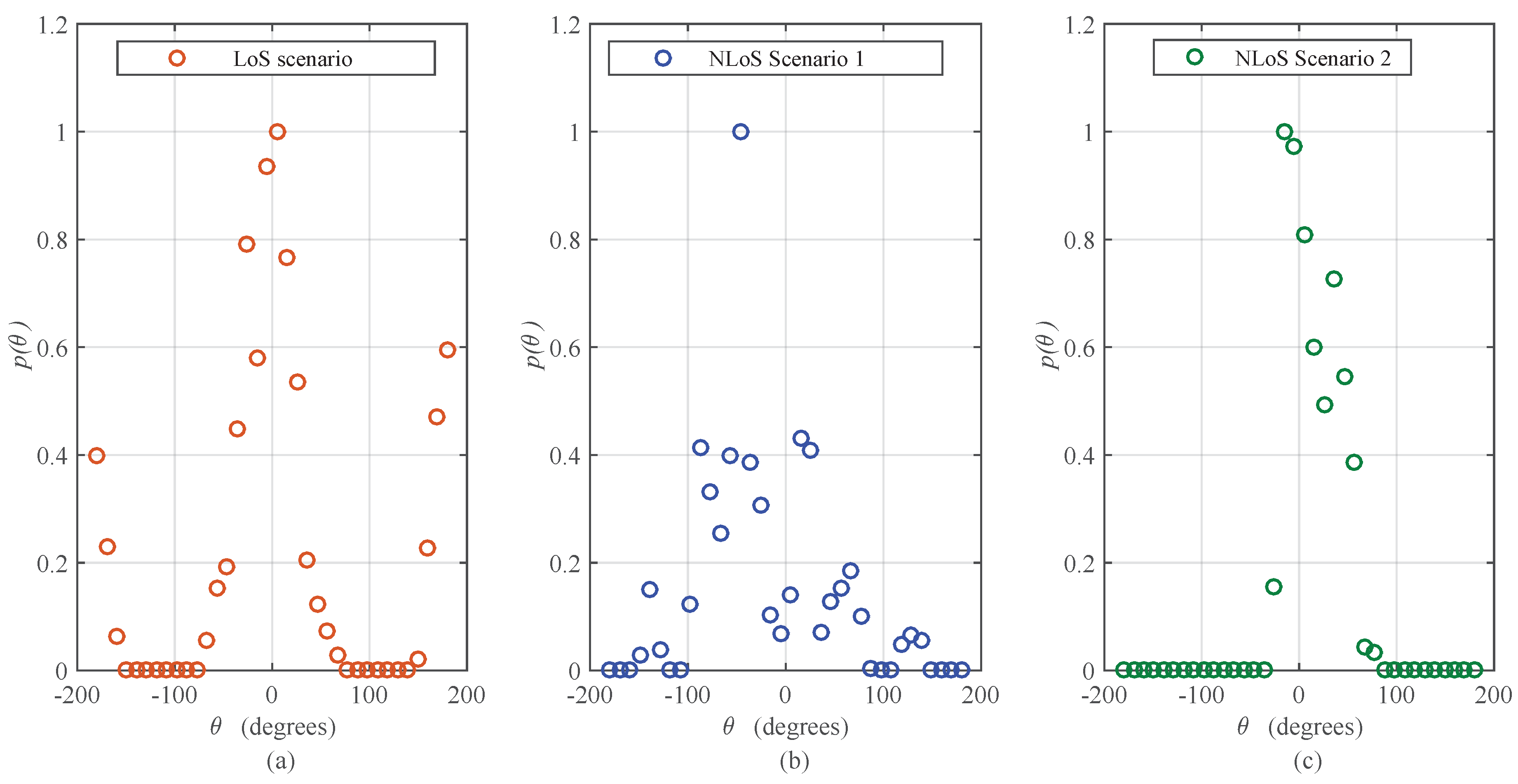
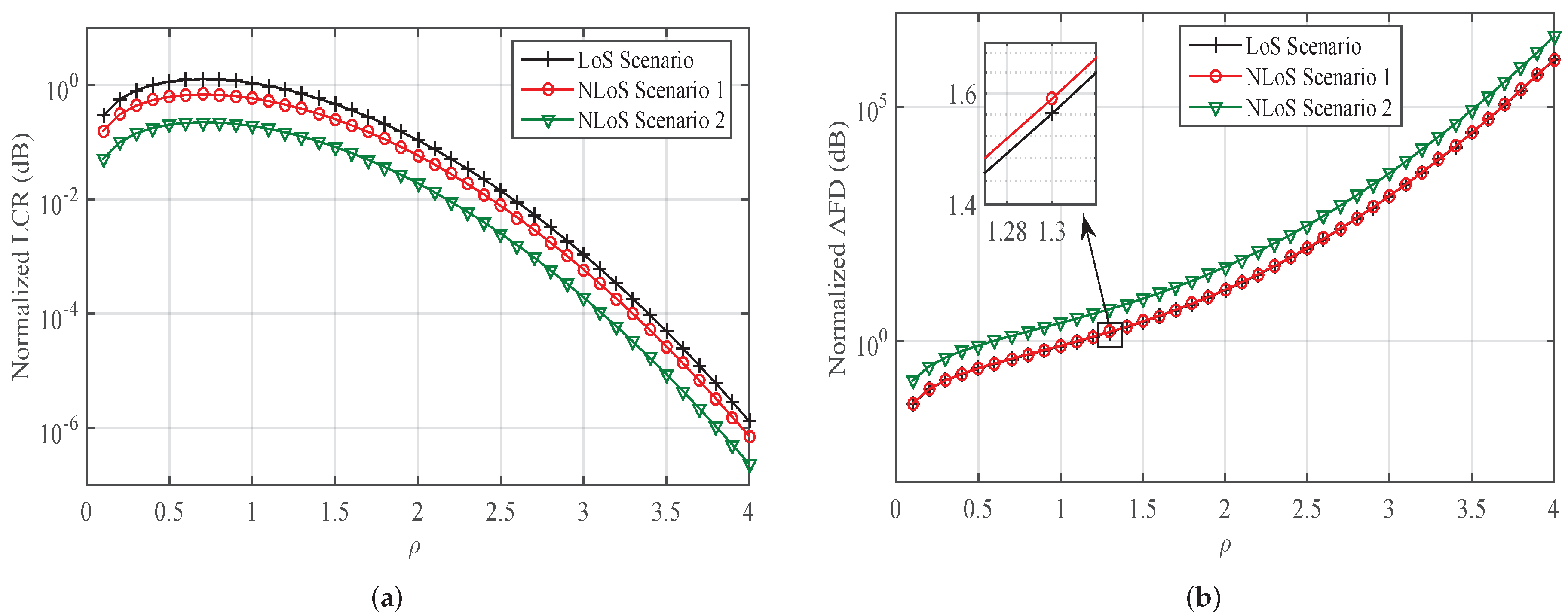
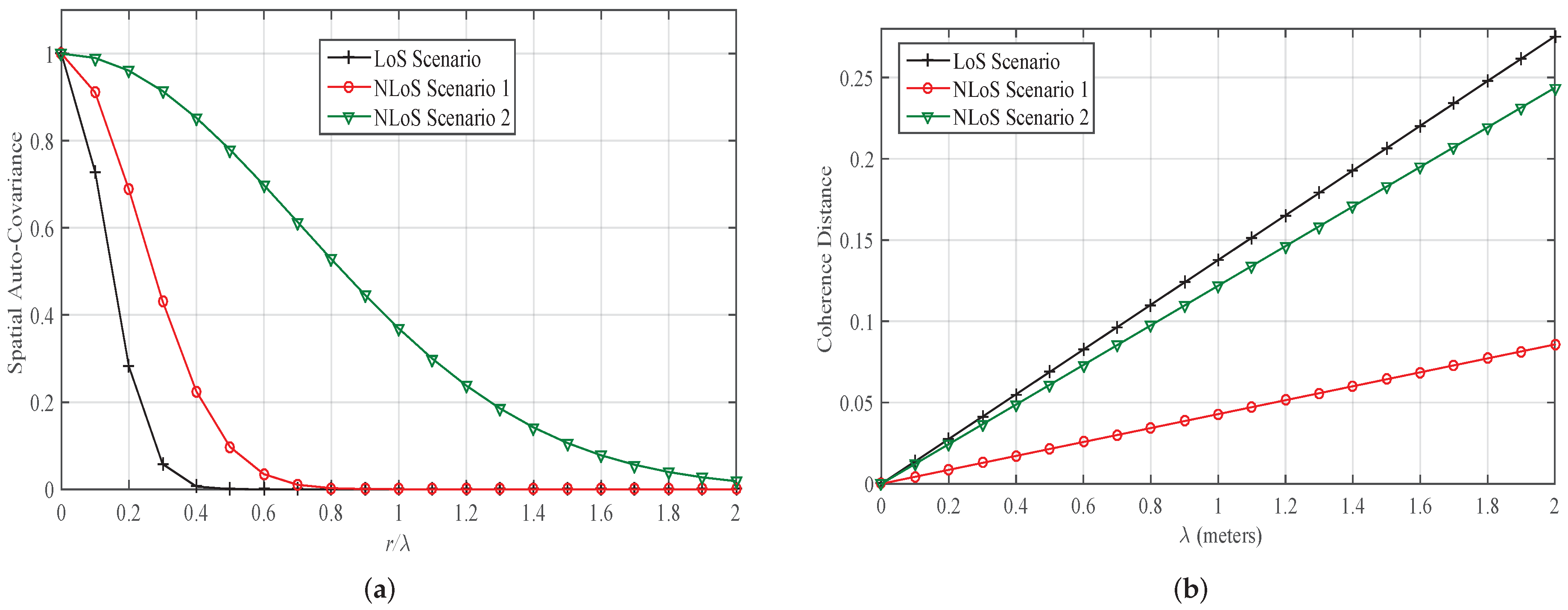
2.3. Case 3: Indoor Office Environment at 28 GHz

In [6], for studying spatial characteristics of 28-GHz mmWave, a channel measurement campaign is conducted in ETRI Daejeon, Korea by using direction scan-sounding in an indoor office environment consists of aligned cubicles offices separated by cardboards and a wide entrance hall and corridors. The Tx was positioned inside the entrance hall and measurements were taken by fixing a transmit horn antenna pointing in the corridor. Three scenarios, a LoS and two NLoS, were considered by changing the location of receiver. The detailed map and measurement setup details are provided in [6]. The measured data is provided as contour-maps for joint azimuth AoA and time-of-arrival (ToA).

2.4. Data Extraction and Calibration

This section explains the methods used to extract the measurement data samples from the graphs published in [4,6,7]. The results of AoA distributions are provided in the form of histogram and scatter plots in [4,7]. The measurement data-sets are extracted by using the “GetData Graph Digitizer” software. The obtained samples in discrete form for angular distribution of multipath power (ADP) with respect to azimuth AoA are then converted from logarithmic to linear scale. After the scale transformation, the discrete data samples are divided with their respective maximum values to set its peak at value 1. This operation is performed to bring uniformity across the different measurement data-sets, for better presentation of the results. The ADP with respect to azimuth AoA for the selected three scenarios of [4] is plotted in Figure 1. The ADP with respect to azimuth AoA for the selected three scenarios for 28 GHz as well as 38 GHz of [7] is plotted in Figure 2. For the results presented in [6] in the form of color-coded contour-maps, we extracted the data samples through image processing tools by using color decoding. Then ADP of azimuth AoA is obtained by numerically integrating the extracted joint data samples of AoA and ToA. All the extracted empirical data-sets are converted from logarithmic to linear scale and then scaled along the vertical axis to fix their peak(s) at 1, which is performed by dividing all the values of a dataset by its peak value. After performing scaling (to set peak at value 1), the ADP of azimuth AoA for the selected three scenarios of [6] is plotted in Figure 3.

3. Channel Statistics

The extracted measurement data for the ADP with respect to azimuth AoA for mentioned environments is represented by $p\left(\theta \right)$, where $\theta$ represents the azimuth direction of signal’s arrival. The quantification of angular spread is conducted by adopting the theory of multipath SFs and definition of true standard deviation proposed in [10,16,17], respectively.

3.1. Definition of Angular Spread Quantifiers

The method to quantify the angle spread is based on Fourier coefficients of ADP with respect to azimuth AoA, $p\left(\theta \right)$. Trigonometric moments are used for calculating the statistics of directional data. The definition of quantifiers used to gauge the spread in dispersion of energy in angular domain is presented in

Table 2. Quantification of Angular Spread for mmWave outdoor and indoor radio propagation channels.

Angular Spread Quantifiers	Quantifiers and Measurement Details	Angular Spread [10]	True Standard Deviation [16,17]	Angular Constriction [10]	Direction of Maximum Fading [10]
	Mathematical Expression:	${\mathrm{\Lambda }}_{\theta }=\sqrt{1-|{\overline{R}}_1{|}^2}$	${\sigma }_{\theta }=\sqrt{-2\ln \left(\right|{\overline{R}}_1\left|\right)}$	${\gamma }_{\theta }=\frac{|{\overline{R}}_2-{\overline{R}}_1^2|}{1-|{\overline{R}}_1{|}^2}$	${\theta }_{\mathrm{MF}}=\frac{1}{2}\mathrm{phase}\{{\overline{R}}_2-{\overline{R}}_1^2\}$
	Range of Quantifier:	0∼1.	0∼2$\pi$ ($0^{\circ }$∼${360}^{\circ }$)	0∼1	$-\pi$∼$\pi$ ($-{180}^{\circ }$∼$+{180}^{\circ }$)
	Description:	Denotes concentration of multipaths around a single direction. 0 indicates the concentration of energy around exactly one path, while 1 indicates no bias.	Denotes measure of energy dispersion in angular domain. Measures the spread in true scientific notation, i.e., radians or degrees.	Denotes concentration of multipaths about two directions. 1 indicates the concentration of energy about exactly two paths, while 0 indicates no bias.	Denotes the physical direction of maximum fading in radians.
Case 1: Outdoor Urban Environment at 38 GHz	Tx-Rx separation < 150 m	0.9829	${105.37}^{\circ }$	0.163	${17.59}^{\circ }$
	Tx-Rx separation > 150 m and < 250 m	0.955	${89.6}^{\circ }$	0.0941	$-{1.99}^{\circ }$
	Tx-Rx separation > 250 m	0.891	${72}^{\circ }$	0.0698	$-{13.72}^{\circ }$
Case 2 (a): Indoor Corridor Environment at 28 GHz	Tx-Rx separation = 3 m	0.8463	${64.30}^{\circ }$	0.7297	$-{32.33}^{\circ }$
	Tx-Rx separation = 5 m	0.8789	${69.7}^{\circ }$	0.74	$-{28.5}^{\circ }$
	Tx-Rx separation = 6 m	0.9077	${75.50}^{\circ }$	0.6605	$-{28.65}^{\circ }$
Case 2 (b): Indoor Corridor Environment at 38 GHz	Tx-Rx separation = 3 m	0.767	${54}^{\circ }$	0.705	$-{33.9}^{\circ }$
	Tx-Rx separation = 5 m	0.969	${96.04}^{\circ }$	0.322	${88.8}^{\circ }$
	Tx-Rx separation = 6 m	0.619	${39.82}^{\circ }$	0.852	${32.1}^{\circ }$
Case 3: Indoor Office Environment at 28 GHz	LoS Scenario (Figure 8b of [6])	0.9049	${74.89}^{\circ }$	0.6834	$-{3.27}^{\circ }$
	NLoS Scenario 1 (Figure 8e of [6])	0.7906	${56.75}^{\circ }$	0.3881	${77}^{\circ }$
	NLoS Scenario 2 (Figure 8h of [6])	0.4125	${24.74}^{\circ }$	0.9212	$-{72}^{\circ }$

. The nth complex trigonometric moment of angular energy’s distribution function, $p\left(\theta \right)$, is ${\overline{R}}_n$ which is given as in [17], as,

$${\overline{R}}_n={\overline{C}}_n+j{\overline{S}}_n,$$

(1)

where,

$${\overline{C}}_n=\frac{1}{P_o}{\int }_0^{2\pi }p\left(\theta \right)\cos \left(n\theta \right)\mathrm{d}\theta ,$$

(2)

and

$${\overline{S}}_n=\frac{1}{P_o}{\int }_0^{2\pi }p\left(\theta \right)\cos \left(n\theta \right)\mathrm{d}\theta .$$

(3)

The total power of angular energy’s distribution function, $p\left(\theta \right)$ is equal to $P_o={\int }_0^{2\pi }p\left(\theta \right)\mathrm{d}\theta$. The trigonometric moments can be modified for the case of discrete data samples, which can be given by,

$${\overline{C}}_n=\frac{1}{F_o}\sum _{i=1}^N{f}_i\cos \left(n{\theta }_i\right),$$

(4)

$${\overline{S}}_n=\frac{1}{F_o}\sum _{i=1}^N{f}_i\cos \left(n{\theta }_i\right),$$

(5)

where $F_o={\sum }_{i=1}^N{f}_i$ for $i=1,\dots ,N$ and $f_i$ is the number of occurrences in ${\theta }_i$th angular bin. In characterization of the SFs, only first and second moments are used; while $|.|$ and $\mathrm{phase}\{.\}$ represent the magnitude and phase of a complex number, respectively.

3.2. Characterization of Angular Spread for Outdoor and Indoor Radio Propagation Channels

The computed numerical results for angular constriction, angular spread, direction-of-maximum fading, and true standard deviation for all the four different cases of outdoor and indoor propagation environment at 28 GHz and 38 GHz with three measurement scenarios for each case of AoA are presented in Table 2. In case 1, quantifiers are computed for outdoor urban environment where measurements were taken at 38 GHz. Angular spread is higher when the distance between Tx and Rx is less and standard deviation gives exact measure in degrees. When separation distance is increased above 250 m, the scatterers in vicinity of Tx reduce, therefore, angular constriction is approaching to zero which shows no bias in concentration of multipaths around specific directions. In case 2, angular spread quantifiers are computed for the given AoA measurements in an indoor corridor environment at 28 GHz as well as 38 GHz for three different values of Tx separation from Rx. All these three separation distances are kept for NLoS scenarios. While analyzing the measurements, it can be seen that power of received signal has variations with respect to AoA at different spatial locations. These variations are higher for higher frequencies and this received power is also more sensitive with respect to variation in AoA. Seeing the results in Table 2, the parameter, ${\mathrm{\Lambda }}_{\theta }$, for 28 GHz and 38 GHz computed at 3 m, 5 m and 6 m is observed higher at 5 m than at 3 m for both the considered frequencies. This shows that at 5 m, the channel can be used effectively for providing rich diversity for a multiple antenna system.

In case 3, all the quantifiers are computed for indoor office environment at 28 GHz. Three scenarios are considered for the measured AoA results. For the LoS case, the angular spread is observed as 0.9049, i.e., close to the highest value of 1. This is because, there also exists another dominant path other than the LoS path, which is from the direction exactly opposite from the LoS direction. This leads to the understanding that the receiver is receiving the signals from multiple directions with no clear bias to a single particular direction. For the same case, the angular constriction is observed to have a strong bias in two physical paths, with a dominant value of 0.6834, see Table 2. The true standard deviation follows the similar trend as of angular spread, but it provides a true physical meaning to the quantified spread by measuring it in a true scientific unit, i.e., radians/degrees. In an indoor environment, the high density of scattering objects in the close vicinity of both the communicating nodes results in a wider angular span. A shift in angular spread and true standard deviation is clearly evident in the results, with a shift from LoS to NLoS channel conditions.

3.3. Definition of SOFS Quantifiers

The considered SOFS quantifiers are LCR, AFD, CD, and spatial auto-covariance. Mathematical relationship of SOFS quantifiers with multipath SFs is provided in [10]. The LCR, ${\mathit{N}}_{\mathit{R}}$, measures the count of a signal envelope’s crossings for a given threshold level R within a unit time interval; which can be represented for Nakagami-m distributed envelope as given below,

$${\displaystyle N_R={\int }_0^{\infty }\dot{r}{f}_R(R,\dot{r})d\dot{r}.}$$

(6)

AFD ($\overline{\tau }$) represents the average time duration for which the signal envelope remains below the threshold level R. AFD for Nakagami-m distributed envelope can be defined as below,

$${\displaystyle \overline{\tau }=\frac{1}{N_R}{\int }_0^R{f}_R\left(r\right)dr.}$$

(7)

In various scenarios of propagation environments, different distributions are adopted for modeling envelope R of the received signal. For LoS scenario, when a strong dominant component is present, the envelope follows Rician distribution. However, when there is no single dominant component present, the envelope follows Rayleigh distribution. Due to its suitability and flexibility, to model the fading channels, Nakagami-m distribution is widely used [28]. It has wide range of applicability and other mostly used distributions such as Rayleigh and Rician can easily be deduced as a special case. The PDF of Nakagami-m is given as,

$${\displaystyle f_R\left(r\right)=\frac{2m^m{r}^{(2m-1)}}{\mathrm{\Gamma }\left(m\right)P_{\circ }^m}\exp \left(\frac{-m{r}^2}{P_{\circ }}\right),}$$

(8)

where m is the shape parameter which is greater than 0.5 and $\mathrm{\Gamma }(.)$ is the standard Gamma function. An expression for LCR and AFD can be derived for Nakagami-m distribution by substituting (8) in (6) and (7), respectively. The derived equations for LCR is expressed as,

$${\displaystyle N_R=\frac{\sqrt{2\pi }{\mathrm{\Lambda }}_{\theta }{m}^{(m-1/2)}{\rho }^{(2m-1)}\exp (-m{\rho }^2)\sqrt{1+{\gamma }_{\theta }\cos \left(2({\theta }_v-{\theta }_{\mathrm{MF}})\right)}}{\lambda \mathrm{\Gamma }\left(m\right)},}$$

(9)

where $\lambda =c/f_d$, $f_d=(v/c)\cos {\theta }_v$ is the maximum Doppler frequency, v is the velocity of receiver, ${\theta }_v$ is the direction of receiver motion, c is the speed of light, and $\rho =R^2/P_{\circ }$ is the normalized threshold level of observation. AFD is the measure of the duration a signal spends below a threshold level and relation of AFD for Nakagami-m distribution is shown below,

$${\displaystyle \overline{\tau }=\frac{\lambda \widehat{\gamma }(m,m\rho )\exp \left(m{\rho }^2\right)}{\sqrt{2\pi }{\mathrm{\Lambda }}_{\theta }\sqrt{1+{\gamma }_{\theta }\cos \left(2({\theta }_v-{\theta }_{\mathrm{MF}})\right)}{m}^{(m-1/2)}{\rho }^{(2m-1)}},}$$

(10)

where $\widehat{\gamma }(.,.)$ is the incomplete Gamma function. Another useful measure for characterization of SOFS is spatial auto-covariance, which determines the correlation between the signals received at two different spatial positions. The relationship of spatial auto-covariance with multipath SFs, for Nakagami-m distribution is given in [29], is shown as follows,

$$p(r,{\theta }_v)\approx \exp \left[-\frac{2{\pi }^{2}m{\mathrm{\Gamma }}^2\left(m\right){\mathrm{\Lambda }}_{\theta }^2\left(1+{\gamma }_{\theta }\cos \left(2({\theta }_v-{\theta }_{\mathrm{MF}})\right)\right)}{\left(m{\mathrm{\Gamma }}^2\left(m\right)-{\mathrm{\Gamma }}^2\left(m+\frac{1}{2}\right)\right)}{\left(\frac{r}{\lambda }\right)}^2\right].$$

(11)

It calculates the correlation between signals received at two different positions separated by a distance r. The separation in space for which the channel response remains unchanged (i.e., more than $50\%$ correlated) is termed as CD, denoted by $D_c$. Studying CD is of high significance in terms of spatial diversity and receiver’s design. The expression for CD is derived for Nakagami-m distributed envelopes which is expressed as,

$${\displaystyle D_c\approx \sqrt{\frac{{\lambda }^2\ln \left(2\right)\left(m{\mathrm{\Gamma }}^2\left(m\right)-{\mathrm{\Gamma }}^2\left(m+\frac{1}{2}\right)\right)}{2{\pi }^{2}m{\mathrm{\Gamma }}^2\left(m\right){\mathrm{\Lambda }}_{\theta }^2\left(1+{\gamma }_{\theta }\cos \left(2({\theta }_v-{\theta }_{\mathrm{MF}})\right)\right)}}.}$$

(12)

These analytical relationships can be used to extend the analysis conducted on SFs in Table 2 to study SOFS of outdoor and indoor mmWave band radio propagation environments.

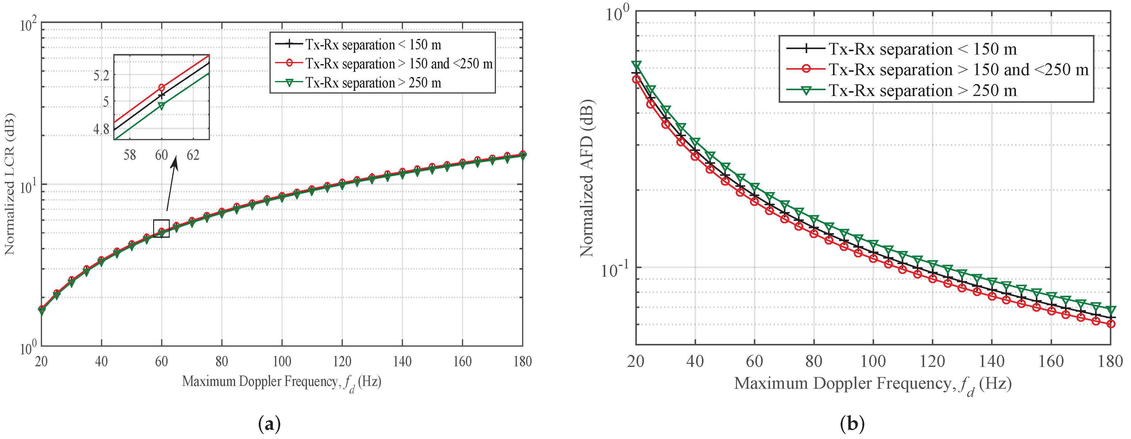
3.4. Characterization of SOFS for Outdoor and Indoor Radio Propagation Channels

The analysis is further extended to study the SOFS of mmWave band channels at 28 GHz and 38 GHz. The impact of change in the maximum Doppler shift, received signal’s envelope’s threshold level and wavelength on the LCR, AFD, spatial auto-covariance, and CD are studied in this section. The Nakagami model is used to approximate the PDF of the power of a Rician fading signal as well as Rayleigh fading signal. For the scenario, where the dominant LoS component is present, the Nakagami shape parameter m is taken as half of ratio of LoS power and NLoS power. In case where dominant component is absent, Rayleigh fading occurs, shape parameter m is taken as one. For Case 1, when the measurement setup is outdoor urban environment and measurements are taken at 38 GHz, the normalized LCR and AFD are plotted in Figure 4a,b, respectively for different values of maximum Doppler frequency. Impact of changing the separation distance between the Tx and Rx on SOFS is studied. It is observed that LCR is increasing with increase in the Doppler frequency, but the change of separation distance has minor impact on LCR. For the AFD case at 38 GHz, it has converse behavior with respect to LCR. AFD is decreasing with increase in maximum Doppler frequency. Moreover, change in separation distance of Tx and Rx has clear impact on AFD which is observed as increasing while distance is kept higher than 250 m. Similarly, for the same Case 1, when the measurement setup is outdoor urban environment and measurements are taken at 38 GHz, the spatial auto-covariance and CD are plotted in Figure 5a,b, respectively for different values of wavelength and distance. Impact of changing the separation distance between the Tx and Rx on these SOFS is studied. It is observed that auto-covariance is decreasing from 1 to 0 when $\frac{r}{\lambda }$ is increased from 0 to 0.5 and then it remains constant at 0 for further increase. However, the change of separation distance has minor impact on auto-covariance. For the CD case at 38 GHz, it has converse behavior with respect to auto-covariance. CD increases linearly with increase in $\lambda$. Moreover, change in separation distance of Tx and Rx has clear impact on CD which is observed as increasing while distance is changed from 150 m to 250 m.

For Case 2 (a), when the measurement setup is indoor corridor environment and measurements are taken at 28 GHz, the normalized LCR and AFD are plotted in Figure 6a,b, respectively for different values of maximum Doppler frequency. Impact of changing the separation distance between the Tx and Rx on SOFS is studied. It is observed that LCR is increasing while we increase the Doppler frequency as well as the change of separation distance has significant impact on LCR. When the distance between Tx and Rx inside corridor is changed from 3 m to 6 m, LCR is observed to increase. For the indoor case at 28 GHz, AFD has converse behavior with respect to LCR. AFD is decreasing with increase in maximum Doppler frequency. Moreover, change in separation distance of Tx and Rx has clear impact on AFD which is observed as decreasing while distance between Tx and Rx inside corridor is changed from 3 m to 6 m. Similarly, for the same Case 2 (a), when the measurement setup is indoor corridor environment and measurements are taken at 28 GHz, the spatial auto-covariance and CD are plotted in Figure 7a,b, respectively for different values of wavelength and distance. Impact of changing the separation distance between the Tx and Rx on these SOFS is studied. It is observed that auto-covariance is decreasing from 1 to 0 when $\frac{r}{\lambda }$ is increased from 0 to 0.5 at 3 m and then it remains constant at 0 for further increase in $\frac{r}{\lambda }$. In addition, the change of separation distance has significant impact on auto-covariance, as it is observed auto-covariance is decreasing from 1 to 0 when $\frac{r}{\lambda }$ is increased from 0 to 0.4 at 6 m. For the CD in indoor case at 28 GHz, it has converse behavior with respect to auto-covariance. CD increases linearly with increase in $\lambda$. Moreover, change in separation distance of Tx and Rx has clear impact on CD which is observed as increasing while distance is changed from 3 m to 5 m and CD has interesting fact that while changing the separation distance from 5 m to 6 m, it is again decreasing. This shows that at 5 m, the channel can be used effectively for providing rich diversity for a multiple antenna system.

For Case 2 (b), when the measurement setup is indoor corridor environment and measurements are taken at 38 GHz, the normalized LCR and AFD are plotted in Figure 8a,b, respectively for different values of maximum Doppler frequency. Impact of changing the separation distance between the Tx and Rx on SOFS is studied. It is observed that LCR is increasing while we increase the Doppler frequency as well as the change of separation distance has significant impact on LCR. When the distance between Tx and Rx inside corridor is changed from 3 m to 5 m, LCR is observed to increase and with further increase in distance up to 6 m, LCR is decreasing. For the indoor case at 38 GHz, AFD has converse behavior with respect to LCR. AFD is decreasing with increase in maximum Doppler frequency. Moreover, change in separation distance of Tx and Rx has clear impact on AFD which is observed as decreasing while distance between Tx and Rx inside corridor is changed from 3 m to 5 m and with further increase in distance up to 6 m, AFD is increasing. This clearly shows that in an indoor corridor environment at higher frequency such as 38 GHz, the channel can be used effectively at 5 m separation for providing rich diversity for a multiple antenna system. Similarly, for the same Case 2 (b), when the measurement setup is indoor corridor environment and measurements are taken at 38 GHz, the spatial auto-covariance and CD are plotted in Figure 9a,b, respectively for different values of wavelength and distance. Impact of changing the separation distance between the Tx and Rx on these SOFS is studied. It is observed that auto-covariance is decreasing from 1 to 0 when $\frac{r}{\lambda }$ is increased, then it remains constant at 0 for further increase in $\frac{r}{\lambda }$. In addition, the change of separation distance has significant impact on auto-covariance, as it is observed auto-covariance is decreasing from with increase in separation distance up to 5 m and then it increases with further increase in distance up to 6 m. For the CD in indoor case at 38 GHz, it has converse behavior with respect to auto-covariance. CD increases linearly with increase in $\lambda$. Moreover, change in separation distance of Tx and Rx has clear impact on CD which is observed as decreasing while distance is changed from 3 m to 5 m and CD has interesting fact that while changing the separation distance from 5 m to 6 m, it is again increasing.

For the Case 3, when the measurement setup is indoor office environment and measurements are taken at 28 GHz, the normalized LCR and AFD against different values of received signal’s envelope’s threshold level is plotted in Figure 10a,b, respectively. An increase at a slow rate in the LCR can be observed with an increase in the threshold level up to a certain threshold level, and a converse behavior of LCR can be observed for higher values of the threshold level. However, LCR has a smaller value for NLoS scenarios as compared to the LoS scenario, for all the threshold levels. The AFD is observed to increase with an increase in threshold level. Moreover, a lower value of AFD is observed for the LoS scenario as compared to the NLoS scenarios. Spatial auto-covariance is plotted in Figure 11a for the considered three scenarios against the distance in spatial points of observations normalized with the wavelength ($r/\lambda$). The rate of drop in spatial auto-covariance for the LoS scenarios compared to the NLoS scenarios is observed to be higher along an increase in the distance between the spatial positions of observation. CD for different scenarios of indoor mmWave channels is plotted in Figure 11b. The coherence indicates the separation distance between two observation points such that the spatial auto-variance remains at least $50\%$. CD is observed to have higher value for the LoS scenario as compared to the NLoS scenarios. Dissemination of the conducted analysis for the specific scenarios of mmWave channels to the research community shall significantly help in an early convergence to establishing generalization in today’s mmWave channel models [30].

4. Conclusions

An analysis on the dispersion of energy in angular domain and characterization of SOFS of 38 GHz and 28 GHz outdoor and indoor radio propagation channels has been conducted. Plain AoA measurement results conducted for four different scenarios at these frequency bands in outdoor and indoor radio propagation environments have been first extracted from the open literature, and then extended to characterize azimuthal spread and SOFS of the radio channel. The considered quantifiers for SOFS are LCR, AFD, CD, and spatial auto-covariance. A detailed analysis on the impact of under-observation amplitude threshold-level, maximum Doppler frequency, and different envelope distributions on the fading statistics of the radio channel has been conducted. The conducted analysis provides various useful insights into the behavior of mmWave outdoor and indoor radio propagation mechanism. The proposed analysis can further be extended to study the optimal antenna elements separation in multi-antenna systems, modulation schemes, interleaving methods, interference mitigation methods, and channel estimation. Moreover, similar studies for other frequency bands and propagation scenarios of mmWave channels can be conducted to establish a comprehensive and generalized understanding of the fading statistics.

References

1. Vatalaro, F.; Forcella, A. Doppler spectrum in mobile-to-mobile communications in the presence of three-dimensional multipath scattering. IEEE Trans. Veh. Technol. 1997, 46, 213–219. [Google Scholar] [CrossRef]
2. Nawaz, S.J.; Khan, N.M.; Patwary, M.N.; Moniri, M. Effect of directional antenna on the Doppler spectrum in 3-D mobile radio propagation environment. IEEE Trans. Veh. Technol. 2011, 60, 2895–2903. [Google Scholar] [CrossRef]
3. Azar, Y.; Wong, G.N.; Wang, K.; Mayzus, R.; Schulz, J.K.; Zhao, H.; Gutierrez, F.; Hwang, D.; Rappaport, T.S. 28 GHz propagation measurements for outdoor cellular communications using steerable beam antennas in New York city. In Proceedings of the IEEE International Conference on Communications (ICC), Budapest, Hungary, 9–13 June 2013; pp. 5143–5147. [Google Scholar]
4. Rappaport, T.S.; Gutierrez, F.; Ben-Dor, E.; Murdock, J.N.; Qiao, Y.; Tamir, J.I. Broadband Millimeter-Wave Propagation Measurements and Models Using Adaptive-Beam Antennas for Outdoor Urban Cellular Communications. IEEE Trans. Antenn. Propag. 2013, 61, 1850–1859. [Google Scholar] [CrossRef]
5. Eldowek, B.M.; El-atty, S.M.A.; El-Rabaie, E.S.M.; El-Samie, F.E.A. Second-Order Statistics Channel Model for 5G Millimeter-Wave Mobile Communications. Arab. J. Sci. Eng. 2017, 43, 2833–2842. [Google Scholar] [CrossRef]
6. Yin, X.; Ling, C.; Kim, M.D. Experimental Multipath-Cluster Characteristics of 28-GHz Propagation Channel. IEEE Access 2015, 3, 3138–3150. [Google Scholar] [CrossRef] [Green Version]
7. Al-samman, A.M.; Abd Rahman, T.; Azmi, M.H. Indoor Corridor Wideband Radio Propagation Measurements and Channel Models for 5G Millimeter Wave Wireless Communications at 19 GHz, 28 GHz, and 38 GHz Bands. Wirel. Commun. Mob. Comput. 2018, 2018, 6369517. [Google Scholar] [CrossRef]
8. Nawaz, S.J.; Wyne, S.; Baltzis, K.B.; Gulfam, S.M.; Cumanan, K. A tunable 3-D statistical channel model for spatio-temporal characteristics of wireless communication networks. Trans. Emerg. Telecommun. Technol. 2017, 28, e3213. [Google Scholar] [CrossRef]
9. Durgin, G.D.; Rappaport, T.S. Effects of multipath angular spread on the spatial cross-correlation of received voltage envelopes. In Proceedings of the IEEE Vehicular Technology Conference, Houston, TX, USA, 16–20 May 1999; Volume 2, pp. 996–1000. [Google Scholar]
10. Durgin, G.D.; Rappaport, T.S. Theory of multipath shape factors for small-scale fading wireless channels. IEEE Trans. Antenn. Propag. 2000, 48, 682–693. [Google Scholar] [CrossRef]
11. Zajic, A.G.; Stuber, G.L. Three-dimensional modeling, simulation, and capacity analysis of space–time correlated mobile-to-mobile channels. IEEE Trans. Veh. Technol. 2008, 57, 2042–2054. [Google Scholar] [CrossRef]
12. Ziolkowski, C.; Kelner, J.M. Statistical evaluation of the azimuth and elevation angles seen at the output of the receiving antenna. IEEE Trans. Antennas Propag. 2018, 66, 2165–2169. [Google Scholar] [CrossRef]
13. Ziolkowski, C.; Kelner, J.M. Antenna pattern in three-dimensional modelling of the arrival angle in simulation studies of wireless channels. IET Microw. Antennas Propag. 2017, 11, 898–906. [Google Scholar] [CrossRef]
14. Valchev, D.G. Spatial Modeling of Three-Dimensional Multipath Wireless Channels. Ph.D. Thesis, Northeastern University, Boston, MA, USA, 2008. [Google Scholar]
15. Valchev, D.G.; Brady, D. Three-dimensional multipath shape factors for spatial modeling of wireless channels. IEEE Trans. Wirel. Commun. 2009, 8, 5542–5551. [Google Scholar] [CrossRef]
16. Nawaz, S.J.; Khan, N.M.; Ramer, R. 3-D Spatial Spread Quantifiers for Multipath Fading Wireless Channels. IEEE Wireless Commun. Lett. 2016, 5, 484–487. [Google Scholar] [CrossRef]
17. Khan, N.M. Modeling and Characterization of Multipath Fading Channels in Cellular Mobile Communication System. Ph.D. Thesis, School of Electrical Engineering and Telecommunication, University of New South Wales, Sydney, Australia, 2006. [Google Scholar]
18. Lu, J.; Han, Y. Application of multipath shape factors in Nakagami-m fading channel. In Proceedings of the International Conference on Wireless Communications & Signal Processing, Nanjing, China, 13–15 November 2009; pp. 1–4. [Google Scholar]
19. Youssef, N.; Wang, C.X.; Patzold, M. A Study on the Second Order Statistics of Nakagami-Hoyt Mobile Fading Channels. IEEE Trans. Veh. Technol. 2005, 54, 1259–1265. [Google Scholar] [CrossRef] [Green Version]
20. Filho, J.; Yacoub, M. On the second-order statistics of Nakagami fading simulators. IEEE Trans. Commun. 2009, 57, 3543–3546. [Google Scholar] [CrossRef]
21. Loni, Z.M.; Khan, N.M. Analysis of fading statistics in cellular mobile communication systems. J. Supercomput. 2013, 64, 295–309. [Google Scholar] [CrossRef]
22. Gulfam, S.M.; Nawaz, S.J.; Ahmed, A.; Patwary, M.N. Analysis on multipath shape factors of air-to-ground radio communication channels. In Proceedings of the 2016 Wireless Telecommunications Symposium (WTS), London, UK, 18–20 April 2016; pp. 1–5. [Google Scholar]
23. Gulfam, S.M.; Nawaz, S.J.; Ahmed, A.; Patwary, M.N.; Ni, Q. A Novel 3D Analytical Scattering Model for Air-to-Ground Fading Channels. Appl. Sci. 2016, 6, 207. [Google Scholar] [CrossRef]
24. Ahmed, A.; Nawaz, S.J.; Gulfam, S.M. A 3-D Propagation Model for Emerging Land Mobile Radio Cellular Environments. PLoS ONE 2015, 10, e0132555. [Google Scholar] [CrossRef]
25. Waseer, W.I.; Junaid Nawaz, S.; Gulfam, S.M.; Mughal, M.J. Second-order fading statistics of massive-MIMO vehicular radio communication channels. Trans. Emerg. Telecommun. Technol. 2018, 29, e3487. [Google Scholar] [CrossRef]
26. Iqbal, T. Statistical Fading Analysis of Millimeter Waves for Mobile Channel. Master’s Thesis, Department of Electronic Engineering, Mohammad Ali Jinnah University, Islamabad, Pakistan, 2015. [Google Scholar]
27. Gulfam, S.M.; Nawaz, S.J.; Baltzis, K.B. Characterization of second-order fading statistics of 28 GHz indoor radio propagation channels. In Proceedings of the 7th International Conference on Modern Circuits and Systems Technologies (MOCAST), Thessaloniki, Greece, 7–9 May 2018; pp. 1–4. [Google Scholar]
28. Nawaz, S.J.; Ahmed, A.; Wyne, S.; Cumanan, K.; Ding, Z. 3-D Spatial Modeling of Network Interference in Two-Tier Heterogeneous Networks. IEEE Access 2017, 5, 24040–24053. [Google Scholar] [CrossRef]
29. Chen, Y.; Mucchi, L.; Wang, R.; Huang, K. Modeling Network Interference in the Angular Domain: Interference Azimuth Spectrum. IEEE Trans. Commun. 2014, 62, 2107–2120. [Google Scholar] [CrossRef] [Green Version]
30. Jameel, F.; Wyne, S.; Syed, J.N.; Chang, Z. Propagation Channels for mmWave Vehicular Communications: State-of-the-art and Future Research Directions. arXiv, 2018; arXiv:1812.02483. [Google Scholar]
Figure 1. Angular distribution of multipath power with respect to azimuth angle of arrival (AoA) for different outdoor mmWave (38 GHz) radio propagation environments; obtained after data calibrations, and normalization operations performed on the measurement results provided in [4]. (a) Tx-Rx separation < 150 m; (b) Tx-Rx separation > 150 and < 250 m; (c) Tx-Rx separation > 250 m Figure 7 of [4].
Technologies 07 00009 g001
Figure 2. Angular distribution of multipath power with respect to azimuth AoA for different mmWave (38 GHz and 28 GHz) indoor corridor environments; obtained after data calibrations, and normalization operations performed on the measurement results provided in [7]. (a) Tx-Rx separation = 3 m; (b) Tx-Rx separation = 5 m; (c) Tx-Rx separation = 6 m Figure 13 of [7].
Technologies 07 00009 g002
Figure 3. Angular distribution of multipath power with respect to azimuth AoA for different indoor mmWave (28 GHz) radio propagation environments; obtained after performing numerical integration along delay domain, data calibrations, and normalization operations on the measurement results provided in [6]. (a) LoS Scenario, Figure 8b of [6]; (b) NLoS Scenario 1, Figure 8e of [6]; (c) NLoS Scenario 2, Figure 8h of [6].
Technologies 07 00009 g003
Figure 4. Level-crossing-rate (LCR) and average fade duration (AFD) plotted against different values of maximum Doppler shift in (a,b), respectively; for different scenarios of outdoor mmWave (case 1; 38 GHz) radio propagation environments. (m = 1, ρ = 2).
Technologies 07 00009 g004
Figure 5. Spatial auto-covariance and coherence distance (CD) for different scenarios of outdoor mmWave (case 1; 38 GHz) radio propagation environments in (a,b), respectively. (m = 1, f d = 1 Hz).
Technologies 07 00009 g005
Figure 6. LCR and AFD plotted against different values of maximum Doppler shift in (a,b), respectively; for different scenarios of indoor mmWave (Case 2 (a); 28 GHz) radio propagation environments. (m = 1, ρ = 2).
Technologies 07 00009 g006
Figure 7. Spatial auto-covariance and CD for different scenarios of indoor mmWave (Case 2 (a); 28 GHz) radio propagation environments in (a,b), respectively. (m = 1, f d = 10 Hz).
Technologies 07 00009 g007
Figure 8. LCR and AFD plotted against different values of maximum Doppler shift in (a,b), respectively; for different scenarios of indoor mmWave (Case 2 (b); 38 GHz) radio propagation environments. (m = 1, ρ = 2).
Technologies 07 00009 g008
Figure 9. Spatial auto-covariance and CD for different scenarios of indoor mmWave (Case 2 (b); 38 GHz) radio propagation environments in (a,b), respectively. (m = 1, f d = 10 Hz).
Technologies 07 00009 g009
Figure 10. LCR and AFD plotted against different values of threshold levels in (a,b), respectively; for different scenarios of indoor mmWave (Case 3; 28 GHz) radio propagation environments. (m = 4 for LoS Scenario and m = 1 for NLoS Scenarios, f d = 1 Hz).
Technologies 07 00009 g010
Figure 11. Spatial auto-covariance and CD for different scenarios of indoor mmWave (Case 3; 28 GHz) radio propagation environments in (a,b), respectively. (m = 4 for LoS Scenario and m = 1 for NLoS Scenarios, f d = 10 Hz).
Technologies 07 00009 g011