Optimization of Machine Process Parameters in EDM for EN 31 Using Evolutionary Optimization Techniques


Department of Mechanical Engineering, BIT, Mesra, Ranchi 835215, India
*
Author to whom correspondence should be addressed.
Technologies 2018, 6(2), 54; https://doi.org/10.3390/technologies6020054
Submission received: 7 May 2018
/
Revised: 30 May 2018
/
Accepted: 4 June 2018
/
Published: 5 June 2018
Abstract
:Electrical discharge machining (EDM) is a non-conventional machining process that is used for machining of hard-to-machine materials, components in which length to diameter ratio is very high or products with a very complicated shape. The process is commonly used in automobile, chemical, aerospace, biomedical, and tool and die industries. It is very important to select optimum values of input process parameters to maximize the machining performance. In this paper, an attempt has been made to carry out multi-objective optimization of the material removal rate (MRR) and roughness parameter (Ra) for the EDM process of EN31 on a CNC EDM machine using copper electrode through evolutionary optimization techniques like particle swarm optimization (PSO) technique and biogeography based optimization (BBO) technique. The input parameter considered for the optimization are Pulse Current (A), Pulse on time (µs), Pulse off time (µs), and Gap Voltage (V). PSO and BBO techniques were used to obtain maximum MRR and minimize the Ra. It was found that MRR and SR increased linearly when discharge current was in mid-range however non-linear increment of MRR and Ra was found when current was too small or too large. Scanning Electron Microscope (SEM) images also indicated a decreased Ra. In addition, obtained optimized values were validated for testing the significance of the PSO and BBO technique and a very small error value of MRR and Ra was found. BBO outperformed PSO in every aspect like computational time, less percentage error, and better optimized values.
1. Introduction
The definition of the word “machining” has evolved significantly over the last couple of decades. In a broader term, machining can be defined as the process to remove material from a work piece or a process where a piece of material is given desired shape and size through a controlled material removal process. The traditional processes such as milling, turning, grinding, drilling, etc., to remove material through mechanical abrasion, micro chipping, or chip formation. There are many reasons due to which the traditional processes are not economical and even possible when hardness of the material to be machined is quite high i.e., above 400 HB, or material is too brittle to be machined, the machining forces are too high for the delicate and slender work piece specimen, the complexity of the part to be machined, and the residual stresses in the machined component which are not at all acceptable [1].
The above disadvantages have led to the development of other material removal mechanisms like mechanical, chemical, thermal, electrochemical, and different hybrid mechanism. These material removal mechanisms have therefore resulted in machining processes referred to as non-traditional machining processes. Owing to advantages offered by the non-traditional machining processes, these are available for an extensive range of industrial applications. The source of energy used differ from process to process and therefore can be categorised accordingly: thermal & electro-thermal processes like laser beam machining, ion beam machining, electric discharge machining etc.; chemical and electrochemical processes such as electrochemical machining, electro-chemical honing, etc.; mechanical processes for instance ultrasonic machining water jet machining, etc.; and hybrid processes such as abrasive EDM, etc.
Electrical discharge machining (EDM), also termed as die sinking, spark machining, wire burning, spark eroding, or wire erosion, is a non-traditional (non-conventional) manufacturing process where a desired shape is obtained with the help of electrical discharges (sparks) [2]. Now-a-days, EDM is a commonly used non-conventional machining process because of its of applications to produce complex shapes with ease, and components which require excellent surface finish which can be used in biomedical, automobile, chemical, aerospace, and tool and die industries to name a few. EDM also offers other advantages such as production of tapered holes, fines holes, delicate components, weak materials machining, and also machining of small work pieces which might get damaged on machining with conventional tool cutting because of their high cutting tool pressure.
In EDM process, both work piece and the tool electrode are submerged inside a dielectric fluid. During machining, a spark channel is generating in between the electrode and work piece gap with generation of very high temperature of about 10,000 °C. This high temperature is sufficient to melt and vaporizes small amount of material from the work piece surface that leads to the material removal from the work piece surface.
2. Need for Optimization
In this modern era of digitalization of technologies and global competitiveness, enterprises and industries need to reduce time and save money and the only way they see it is through optimization of process parameters. EDM process suffers from a number of limitations such as higher power consumption, high cost on initial investment and large floor space. Further, it can machine only conductive materials and is more expensive when compared to a traditional process like milling and turning. Therefore, a careful selection of the different parameters and careful planning is recommended before commencing the machining process. Selection of suitable machining parameters is critical to achieve optimum machining results. Many researchers and academicians have tried performing optimization for various manufacturing processes (both conventional and non-conventional) through traditional and non-traditional optimization methods considering various process parameters to obtain optimum results. For EDM, MRR (Material Removal Rate), and Ra (Roughness Parameter, average roughness) are considered as the most important parameters and the need to maximize MRR and minimize Ra has always been the goal for many researchers and industries.
3. Literature Survey
To find an optimized set of inputs for achieving appropriate outputs has always been a challenge and a tedious task for researchers for many years. Effects of EDM process parameters on machining responses or performances has been studied by many researchers. However, machining performances and responses considered, relationship between different process parameters and machining responses and also optimization techniques used by different researchers are quite diverse. For modelling the mathematical relationship between machining responses and process parameters, there have been different techniques that have been used by different researchers but the one that is mostly used and preferred for the EDM process is second order polynomial model or response surface model (RSM) [3,4,5,6,7,8,9,10]. Though response surface model is simple for implementing, there is a very big error of estimation value in this technique when responses are nonlinear. Many other techniques like Artificial Neural Network (ANN) [3,11,12], which supports vector machine regression [13], and adaptive neuro-fuzzy interference have also been used by researchers in the past [14]. Though when compared with SRM models or conventional polynomials these regression model has found to be better than that. Kriging model developed in geostatic in South Africa is also being used to define the relationship between different process parameters and machining responses in EDM, and it has been found to be better than both SRM and ANN when highly nonlinear characteristic and efficiency in cost [15] of experimentation is considered though Kringing model may require more points to capture non-linear behaviour [16,17]. When optimizing the process parameters, it helps an EDM operator to get the most optimum machining outputs for a required purpose. There are other methods that have been also been used for optimization of EDM machining such as Taguchi [18,19,20,21,22,23], genetic algorithm [3,11,12,24], and TOPSIS (Technique for Order of Preference by Similarity to Ideal Solution) [5,25]. Taguchi uses signal to noise ratio for reaching optimal level of process parameters though the flaw in this method is that it does not promises ‘real optimal’ solution since it only addresses the discrete control factors or design variables [26]. TOPSIS, is simply a multi-criteria decision making method, and is not a standard mathematical optimization technique and does not promise real optimal solution. Genetic Algorithm is a quite popular optimization technique having many engineering applications [27].Khalid proposed the idea of EDiMfESO (Electrical Discharge Machine using Fuzzy Fitness Evolutionary Strategies Optimization) and he successfully optimized MRR, Ra, and Tool Wear Rate (TWR) [28]. This technique uses evolutionary strategy (ES) combined with dynamic fuzzy to predict the most appropriate multi-objective optimization setting for carrying out operation in EDM. Lin et al., used Grey-Taguchi technique to obtain multiple performance characteristics like high MRR, low working gap and low electrode wear when machining with Inconel 718 alloy [29]. Similarly, Tang & Du performed operation on EDM in tap water on Ti–6Al–4Vusing Taguchi technique and Grey Relational Analysis technique and tried to optimize the process parameters and presented a comparative analysis on using tap water with dielectric fluids [30]. Aliakbari and Baseri optimized machining parameters in the rotary EDM process with the help of the Taguchi technique [31].
4. Research Gap
It can be observed from the above literature survey that traditional methods such as graphical solution technique, Taguchi, TOPSIS, etc. have mostly been used for the parametric optimization of the EDM process. However, the traditional methods are restricted over a broad range of spectrum of problem domains. The complexity of the optimization problem further limits the application of the traditional optimization methods. The use of non-traditional methods such as GA (Genetic Algorithm) provides a near optimal solution. Therefore, to overcome the drawbacks of the traditional optimization techniques and non-traditional methods such as GA, PSO, ABC (Ant Bee Colony), and other heuristic and evolutionary optimization techniques are being used by the scientific community. The evolutionary optimization algorithm is based on biological genetics. These optimization techniques are more robust in comparison to the traditional techniques because instead of making use of functional derivatives, fitness information is used by the evolutionary optimization techniques. Therefore, efforts are being made to use such optimization techniques to achieve a more accurate solution.
Therefore, in this research paper, PSO was adopted for the optimization of Ra and MRR for the EDM of EN31. Pulse Current (A), Gap Voltage (V), Pulse on time (µs), and Pulse off time (µs) are considered as the process parameters. Further, the multiple-objective optimization is performed for the Ra and MRR through PSO. The PSO technique is compared with BBO technique. A comparative analysis is presented between both the optimization techniques to find out the best optimization technique in terms of computational time, best parameters obtained, less percentage errors, etc.
5. Experimental Setup
Die-Sinking EDM machine (Electronica EMT-43 Machine) was used to conduct the experiments. EDM process was carried out on the work piece EN 31 material having cylindrical cross-section having dimension of 25 mm × 15 mm. The tool for EDM operation was rectangular positive (+) polarity of Copper (Cu) having dimension 25 mm × 25 mm. The dielectric medium chosen was paraffin oil. Before the start of the EDM operation, initial weight of the work piece was measured and it was compared with weight of the work piece after the EDM operation and henceforth the difference in the weight gave us the MRR of EN 31 material. Ra on the machined surfaces were obtained with the Talysurf (Make—Taylor Hobson, Leicester, UK) and were measured on the centre of the workpiece. Table 1 and Table 2 below represents the chemical composition and mechanical properties of the EN 31 tool steel. Table 3 represents the mechanical properties of the electrode. Table 4 shows specification of die sinking EDM machine.
5.1. Input& Output Parameters
5.1.1. Output Parameters
The four input parameters considered for the EDM experimentation are: Pulse Current (A); Pulse on time (µs); Pulse off time (µs); and Gap Voltage (V).The above parameters were chosen on the basis of extensive literature surveys that have reported these parameters to be most influential for the MRR and the Ra.
5.1.2. Output Parameters
The two output parameters considered were: MRR and Ra.
Material Removal Rate (MRR)
Equation (1) could be used for the determination of the MRR (cubic centimetre/min) in the EDM process:
where, Wi is the initial weight of the work piece before machining, Wf is the final weight of the work piece after machining, and t is the time period of trials.
MRR is directly proportional on the amount of current passed and the machining time (Pulse on Time, Pulse off Time). Besides these critical factors the MRR is also dependent on the type of voltage etc.
Average Roughness (Ra)
The deviation of a surface from its ideal level is defined in terms of surface roughness. The surface roughness is defined according to ISO 4287:1997 international standard. The term average roughness is often referred to as roughness and determines the surface texture. The average roughness is calculated by the deviations, i.e., deviation of surface from a theoretical centre line. If the deviations are large, the surface roughness is high, whereas the surface is considered to be smooth for small deviations. This is known as arithmetic mean surface roughness Ra.
5.2. Experimentation
The experimentation carried out on EDM considering input parameters mentioned above and the output parameters obtained are shown as below in Table 5.
5.3. Regression Model
The relationship between the input parameters and the output parameters can be obtained using the statistical tool of regression analysis. Minitab 16 was used for obtaining the relationship between MRR and input variables and also for obtaining the relationship between Ra and the input variables. Equations (2) and (3) are the relations for MRR and Ra respectively.
MRR = 0.000253A + 0.011500B + 0.008014C − 0.250000D + 0.058007
Ra = 0.0254A + 1.3904B + 0.3726C + 0.5101D + 2.0411.
Here, A has been substituted for are Pulse Current (A), B for Pulse on time (µs), C for Pulse off time (µs), and D for Gap Voltage (V).
5.4. PSO Technique
Kennedy and Eberhart [32] developed the PSO technique which is one of the evolutionary (heuristic) optimization techniques. The common evolutionary computational attributes exhibited by the PSO technique simulates graphically the choreography of the bird flock. The PSO technique incepts with the initialization with population of random solution and then updating the generations to achieve the optimal solution. The potential solutions which are referred to as particles are then flown through the space of the problem which follows the current optimum solution. The particles in the problem space keeps track of its position. The coordinate of each particle is associated with the best solution achieved so far. The best position achieved by the particle is referred to as ‘pBest’. The best position achieved by any particle in the problem space is known as the ‘gBest’. Thus the PSO technique is based on accelerating the particles towards their ‘pBest’ and ‘gBest’ locations. The random terms weight the acceleration and therefore separate set of random numbers are generated for acceleration towards ‘gBest’ and ‘pBest’. The updated velocity i.e., the new velocity of the particle is obtained using the Equation (4). Equation (5) on the other hand gives the updated position of the particle in the problem space.
The random numbers r1 and r2 are generated randomly and lie in the range [0, 1]. c1 and c2 are the acceleration constants that weights the acceleration terms. The confidence of the particle in itself is represented by c1 whereas c2 represents the confidence a particle has in a swarm. c1 and c2 are referred to as cognitive and social parameters, respectively. The values of these two parameters determines the change in amount of tension in the system. The low values of the parameters result in the particles roaming far away from the target regions whereas a higher value results in an abrupt movement towards the target solution [33]. The exploration abilities of the swarm particles are controlled by the inertia weight w and is therefore very critical in determining the convergence behaviour of PSO. The lower values of w restrict the velocity updates to nearby region in the search space, whereas higher values result in velocity updates for a wider space in the problem space. Berg and Engelbrecht [34] have investigated the effect on convergence if benchmark functions of w, c1, and c2.
Heuristics have been developed to obtain the values of c1, c2, and w but these are applicable for single-objective optimization problems only. Determination of the parameters and the inertia weights for multi-objective optimization problems is relatively difficult and therefore a time variant of PSO has been described by Tripathi et al. [35]. In this variant of PSO, the parameters and the inertia weights are adaptive and changes with the iterations. The search space can be explored more efficiently with the adaptive nature of the time variant PSO technique. The premature convergence was taken care off by the mutation operator.
The PSO technique doesn’t require complex encoding and decoding process as required by genetic algorithm. The real number represents a particle which update their internal velocity in search of the best solution. In PSO technique the particles tend to converge towards the best solution by iteratively looking for the best position which comprises of the evolution phase. It is very important to handle the non-linear equation constraints and evaluate the infeasible particles. This is mainly due to the fact that the particles generated during the process may violate the constraints of the system and thereby resulting in infeasible particles. Various approaches such as repair of infeasible particles, rejection of the infeasible particles, penalty function methods etc. can be adopted to cope with the evolutionary problems with constraints. The recent developments however suggest the use of penalty method for addressing the same [33].
5.5. BBO Technique
The BBO technique was initially introduced by Dan Simon [36] in the year 2008, who is a professor at Cleveland State University in the department of Electrical and Computer Engineering. BBO falls into the category of evolutionary optimization techniques in heuristic based optimization techniques and it tries to optimize a function stochastically and through iteration trying to improve a candidate’s solution through fitness function or given measure of quality quite similar to PSO technique. Like many other evolutionary optimization techniques BBO drew its inspiration from nature. It is based on the study of distribution of species or speciation (the evolution of new species), the migration of species between islands, and the extinction of species.
This algorithm is based on a mathematical model, describing the migration of species between habitats, in the form of emigration from non-suitable habitats and immigration to suitable habitats. The suitability of habitats, is computed and stored as Habitat Suitability Index (HSI), and its definition is completely related to the objective function of the optimization problem, being solved. The HSI (Habitat Suitability Index) here is the fitness value similar to the one in PSO.
The concept of BBO can be understood as follows:
An island which has higher suitability will have large or more number of species living in them compared to that of an island which has low suitability and henceforth the number of species living in them will be low. The suitable island for species will therefore be having High Suitability Index (HSI) and variables characterizing HSI are called as Suitability Index Variable (SIV). Hence in a habitat the SIVs are the independent variables whereas HSIs are the dependent variables.
An island having a higher number of HSI will be having more number of species and henceforth will be having high number of emigration rate and low immigration rate. HSI would tend to be static. Species will move to the nearest island since they have high emigration level and vice-versa. Now, species which have immigrated to another island would not disappear from their origins completely and such species will appear to be present at both islands at same time. Hence, migration process would make the bad solution accept some features from the better solutions. Apart from the migration process, mutation and elitism also takes place in BBO. Mutation rate is the probability of mutation on few habitats. Islands which will be having high HSI will have a low mutation rate and similarly islands with low HSI will have a high mutation rate compared to the previous one. Henceforth, a good solution is barely chosen to be mutated because of the fact that it can last until the next generation. This mutation will replace the old habitat having low HSI rate with new habitat. Solutions having low HSI would be more dominant if there is no mutation so that they can easily be trapped to the local optima. Rate of mutation can be calculated as follows from Equation(6) below:
where,
- mk = mutation rate,
- mmax = maximum mutation rate,
- Pk = probability of number of species,
- Pmax = maximum probability,
New habitat from mutation will replace the old habitat and with elitism best solution found earlier would continue to remain. Mutations might take place on all the solutions except the one having best solution with the highest probability (Pk).
Let us consider at time t, the recipient island has S species with probability PS(t), and λS and µS are consecutively the immigration and emigration rates at the presence of S species on that particular island. Then the variation from PS(t) to PS(t + Δt) can be described in Equation(7) below:
Thus, using the known values of PS(t) and S(t), the value of Ps(t + Δt) given in Equation (7) can be approximated as:
The above equation (Equation (8)) will be used in the programming of BBO for calculating PS(t + Δt). The algorithm for the BBO is shown below in Figure 3:
6. Optimization of Mrr and Ra Using PSO and BBO
The PSO technique incepts with the setting of PSO parameters which determines the performance of the PSO algorithm. The values of parameters were taken from the work of Hu and Eberhart [37]. Therefore, w = 0.5 + (rand/2), c1 = c2 = 1.49445, number of iterations =100 and population size = 50 particles.
As a second step to PSO technique, initialization of the random position and velocity vectors is followed. The fitness values are derived from the following function given by Equation (9):
f1 and f2 are normalized values of MRR and Ra. The values of inertia weights considered are 0.5 for MRR and 0.5 for Ra as we have given equal importance to both the parameters. The initial values have been tabulated in the Table 6.
Finding pBest and gBest is a third step to the PSO technique. The lowest fitness value is selected as the gBest and for the first iteration the pBest will be same as gBest. The change in position is then obtained using Equations (4) and (5) for each of the parameters. Table 8 shows the new position of particles after first iteration and the change in position of each particle has been tabulated in the Table 7.
As can be observed from Table 8, particle 2 has the minimum Fitness Value. Therefore, the pBest for each parameter will be the values corresponding to particle 2. However, it is higher than the initial gBest. Hence the gBest achieve is not updated. The process is continued for 100 iterations and the final optimised value of gBest gives the final solution.
A similar process was adopted for the multiple objective optimization using BBO. The HSI or fitness value was calculated and similar to PSO the best values were updated after each iteration and the iteration is continued until the final optimised value is obtained.
7. Results and Discussion
Repeating the above steps of PSO until the termination condition takes place (maximum number of iterations) we get the optimised value of MRR and Ra. Final values in the corresponding dimensions of the particle, i.e., GbestA = 40, GbestB = 110, GbestC = 230, GbestD = 50 (GBEST archive), are selected as optimal values. The values corresponding to the optimised value of MRR & Ra for the various input parameters are: A = 40; B = 110; C = 230; D = 50. MRR obtained through these parameters 235 mm3/min and Ra is 18.4 µm.
Similarly, running the algorithm for BBO technique until the termination condition takes place (maximum number of iterations) we get the optimised value of MRR and Ra. Final values in the corresponding dimensions of the particle, are selected as optimal values. The values corresponding to the optimized MRR & Ra for the various input parameters are: A = 40; B = 100; C = 210; and D = 50. MRR 242 mm3/min and Ra 17.98 µm were obtained using these parameters.
Figure 4 below shows the 3D contour graphs of the relation between different input and output process parameters. It can be clearly inferred from the graph that when current is increased MRR and Ra increases linearly with the current, however, when the value of current is very large or low MRR and Ra shows non-linearity and increases slowly. It can be explained with the phenomenon that when current is low, amount of heat generating from the spark entering work piece is also very small and is easily affected by cooling effect of dielectric environment.
When the impacts of various input process parameters and their response or their effects on machining parameters are considered, the global effects of these responses can be understood from Figure 5 given below. It can be clearly observed that Pulse Current has the major impact or effect on MRR as well as Ra. Other parameters, like Pulse on time and Pulse off time, have low effects compared to Pulse Current whereas Gap Voltage has the least effect of all the parameters considered. Because of the duty cycle in EDM (ratio of pulse on time and the total cycle time) it is fairly understood that Pulse on time and pulse off time have considerable impact.
Error in experimental and optimized data for MRR is 1.26% and for Ra it is 1.36 through PSO as shown in Table 9, whereas a relatively low percentage error was obtained using BBO technique gave 0.83% in MRR and 0.166% for Ra which are shown in Table 10. A relatively low percentage error of 1.26% − 0.83% = 0.43% for MRR and 1.63% − 0.66% = 0.97% for Ra was obtained with BBO when compared with PSO. A lower surface roughness and a greater MRR was obtained using the BBO technique and that too more accurately.
The surface morphology of the work-piece before machining and after machining is studied using SEM images shown in Figure 6a,b, respectively. It is evident from the Figure 6a that before machining, the work surface is almost smooth and after machining using initial parameters is rough as compare to previous figure. Figure 6c shows the SEM image of the workpiece made by using optimal parameters using BBO where as Figure 6d depicts the same for PSO. It is observed that the surface roughness of optimum condition is better than the initial condition in both cases but between two BBO provides a smoother surface.
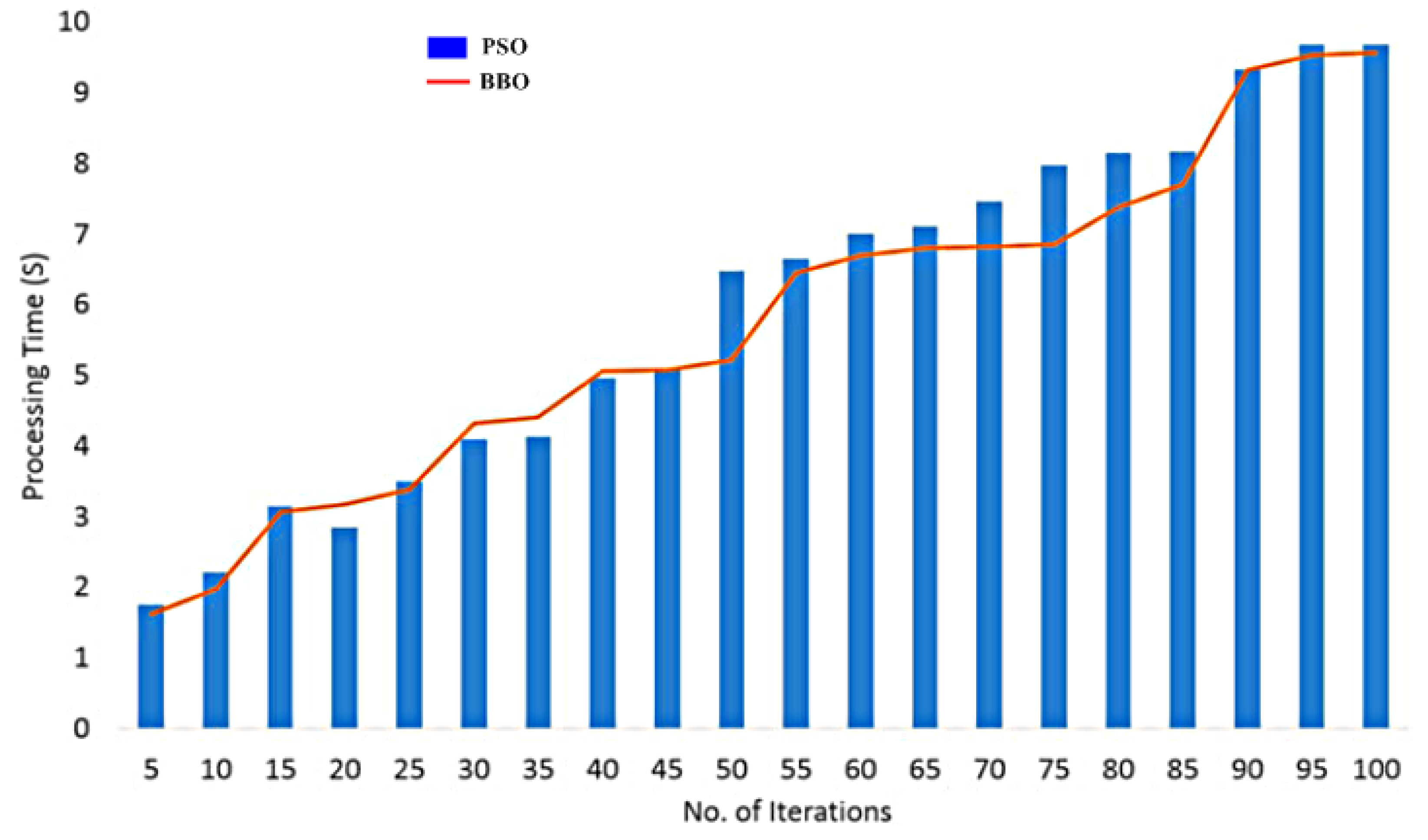
In the current work, 100 runs were carried out in the PSO and BBO algorithms. The PSO reaches a good fitness function as can be observed in Figure 7; in iteration 40 and after that there is no significant improvement. The same can be said for the BBO technique but at an even lower iteration of around 30. Moreover, it can also be concluded, from Figure 8, that the processing time for BBO is less when compared with that of PSO because of the lesser complexity in the BBO algorithm and simple formula to compute fitness or HSI function. Hence BBO is a better choice compared with that of PSO since it requires less computation time which means less production time and henceforth production cost is reduced.
8. Conclusions
In the present paper, the multiple-objective optimization of the MRR and Ra for the EDM process of EN31 was carried out using the PSO and BBO algorithm. The optimum value of MRR and Ra were established. It can beconcluded that the BBO has outperformed PSO in every aspect like having better optimized values with less relative percentage error. Even the computation time was less when in BBO compared with that of PSO. Better optimized values were obtained like greater MRR and less Ra was obtained with BBO which was the main goal of the whole experiment. The solution obtained with PSO and BBO were verified and validated with experimental results. The multiple objective optimization can be used to fulfil the specific requirement of the manufacturing unit. Therefore, the BBO algorithm proved to be a cost effective solution for establishing the optimum values of input process parameters for enhancing the machining performance of the EDM process.
9. Scope of Future Research
PSO and BBO can be further used for multi-objective optimization for MRR and Ra combined with additional responses like EWR (Electrode Wear Ratio), overcut, etc. Further, the optimization can be performed by taking into account more input parameters like flushing pressure, electrode material, etc. The machining optimization of EDM for composite materials can be investigated with PSO and BBO. It would be quite interesting to note how performance of BBO could be compared with other evolutionary optimization techniques like GA, DE, etc. Moreover PSO and BBO algorithm can be used for the optimization of process parameters for other non-conventional machining processes such as ultrasonic machining, Electro Chemical Machining, etc.
Author Contributions
Both authors have contributed equally towards the presented research work.
Acknowledgments
The authors sincerely acknowledge the comments and suggestions of the reviewers that have been instrumental for improving and upgrading the chapter in its final form.
Conflicts of Interest
The authors declare no conflict of interest.
References
- Kalpakjian, S. Manufacturing Processes for Engineering Materials; Pearson Education: Delhi, India, 1984; ISBN 978-8-13170-566-7. [Google Scholar]
- Jameson, E.C. Electrical Discharge Machining; SME: Steyning, UK, 2001; ISBN 978-0-87263-521-0. [Google Scholar]
- Dewangan, S.; Gangopadhyay, S.; Biswas, C.K. Multi-Response Optimization of Surface Integrity Characteristics of EDM Process Using Grey-Fuzzy Logic-Based Hybrid Approach. Eng. Sci. Technol. Int. J. 2015, 18, 361–368. [Google Scholar] [CrossRef]
- Gopalakannan, S.; Senthilvelan, T.; Ranganathan, S. Modeling and Optimization of EDM Process Parameters on Machining of Al 7075-B4C MMC Using RSM. Procedia Eng. 2012, 38, 685–690. [Google Scholar] [CrossRef]
- Hourmand, M.; Farahany, S.; Sarhan, A.A.D.; Noordin, M.Y. Investigating the Electrical Discharge Machining (EDM) Parameter Effects on Al-Mg2Si Metal Matrix Composite (MMC) for High Material Removal Rate (MRR) and Less EWR–RSM Approach. Int. J. Adv. Manuf. Technol. 2015, 77, 831–838. [Google Scholar] [CrossRef]
- Luis, C.J.; Puertas, I.; Villa, G. Material Removal Rate and Electrode Wear Study on the EDM of Silicon Carbide. J. Mater. Process. Technol. 2005, 164, 889–896. [Google Scholar] [CrossRef]
- Majumder, A.; Das, P.K.; Majumder, A.; Debnath, M. An Approach to Optimize the EDM Process Parameters Using Desirability-Based Multi-Objective PSO. Prod. Manuf. Res. 2014, 2, 228–240. [Google Scholar]
- Sánchez, H.; Estrems, M.; Faura, F. Development of an inversion model for establishing EDM input parameters to satisfy material removal rate, electrode wear ratio and surface roughness. Int. J. Adv. Manuf. Technol. 2011, 57, 189–201. [Google Scholar] [CrossRef]
- Joshi, S.N.; Pande, S.S. Intelligent Process Modeling and Optimization of Die-Sinking Electric Discharge Machining. Appl. Soft Comput. J. 2011, 11, 2743–2755. [Google Scholar] [CrossRef]
- Rao, G.K.M.; Rangajanardhaa, G.; Rao, D.H.; Rao, M.S. Development of hybrid model and optimization of surface roughness in electric discharge machining using artificial neural networks and genetic algorithm. J. Mater. Process. Technol. 2009, 209, 1512–1520. [Google Scholar]
- Aich, U.; Banerjee, S. Application of Teaching Learning Based Optimization Procedure for the Development of SVM Learned EDM Process and Its Pseudo Pareto Optimization. Appl. Soft Comput. J. 2016, 39, 64–83. [Google Scholar] [CrossRef]
- Al-Ghamdi, K.; Taylan, O. A Comparative Study on Modelling Material Removal Rate by ANFIS and Polynomial Methods in Electrical Discharge Machining Process. Comput. Ind. Eng. 2015, 79, 27–41. [Google Scholar] [CrossRef]
- Sakata, S.; Ashida, F.; Zako, M. Structural optimization using kriging approximation. Comput. Methods Appl. Mech. Eng. 2003, 192, 923–939. [Google Scholar] [CrossRef]
- Pantula, P.D.; Miriyala, S.S.; Mitra, K. KERNEL: Enabler to Build Smart Surrogates for Online Optimization and Knowledge Discovery. Mater. Manuf. Process. 2017, 32, 1162–1171. [Google Scholar] [CrossRef]
- Miriyala, S.S.; Mittal, P.; Majumdar, S.; Mitra, K. Comparative Study of Surrogate Approaches While Optimizing Computationally Expensive Reaction Networks. Chem. Eng. Sci. 2016, 140, 44–61. [Google Scholar] [CrossRef]
- Muthuramalingam, T.; Mohan, B. Application of Taguchi-Grey Multi Responses Optimization on Process Parameters in Electro Erosion. Measurement 2014, 58, 495–502. [Google Scholar] [CrossRef]
- Nikalje, A.M.; Kumar, A.; Srinadh, K.V.S. Influence of Parameters and Optimization of EDM Performance Measures on MDN 300 Steel Using Taguchi Method. Int. J. Adv. Manuf. Technol. 2013, 69, 41–49. [Google Scholar] [CrossRef]
- Naik, D.V.; Srinivasan, D.R. Multi objective optimization of cutting parameter in EDM using grey taguchi method. Int. J. Sci. Res. 2013, 4, 1091–1095. [Google Scholar]
- Selvarajan, L.; Narayanan, C.S.; Jeyapaul, R. Optimization of EDM Parameters on Machining Si3N4-TiN Composite for Improving Circularity, Cylindricity, and Perpendicularity. Mater. Manuf. Process. 2016, 31, 405–412. [Google Scholar] [CrossRef]
- Rahang, M.; Patowari, P.K. Parametric optimization for selective surface modification in EDM using taguchi analysis. Mater. Manuf. Process. 2016, 31, 422–431. [Google Scholar] [CrossRef]
- Gill, A.S.; Kumar, S. Surface Roughness and Microhardness Evaluation for EDM with Cu–Mn Powder Metallurgy Tool. Mater. Manuf. Process. 2016, 31, 514–521. [Google Scholar] [CrossRef]
- Manivannan, R.; Kumar, M.P. Multi-response optimization of Micro-EDM process parameters on AISI304 steel using TOPSIS. J. Mech. Sci. Technol. 2016, 30, 137–144. [Google Scholar] [CrossRef]
- Salman, Ö.; Kayacan, M.C. Evolutionary programming method for modeling the EDM parameters for roughness. J. Mater. Process. Technol. 2008, 200, 347–355. [Google Scholar] [CrossRef]
- Mitra, K. Genetic algorithms in polymeric material production, design, processing and other applications: A review. Int. Mater. Rev. 2008, 53, 275–297. [Google Scholar] [CrossRef]
- Lin, H.-L.; Chou, C.-P. Optimization of the GTA welding process using combination of the taguchi method and a neural-genetic approach. Mater. Manuf. Process. 2010, 25, 631–636. [Google Scholar] [CrossRef]
- Roy, A.K.; Kumar, K. Effect and Optimization of Machine Process Parameters on MRR for EN19 & EN41 Materials Using Taguchi. Procedia Technol. 2014, 14, 204–210. [Google Scholar]
- Marafona, J.D.; Araújo, A. Influence of workpiece hardness on EDM performance. Int. J. Mach. Tools Manuf. 2009, 49, 744–748. [Google Scholar] [CrossRef]
- Khalid, N.E.A. EDM Using Fuzzy for Fitness Evolutionary Strategies Optimization. In Proceedings of the the 15th WSEAS international conference on Computers, Corfu Island, Greece, 14–16 July 2011; pp. 334–339. [Google Scholar]
- Lin, M.Y.; Tsao, C.C.; Hsu, C.Y.; Chiou, A.H.; Huang, P.C.; Lin, Y.C. Optimization of Micro Milling Electrical Discharge Machining of Inconel 718 by Grey-Taguchi Method. Trans. Nonferrous Met. Soc. China 2013, 23, 661–666. [Google Scholar] [CrossRef]
- Tang, L.; Du, Y.T. Experimental Study on Green Electrical Discharge Machining in Tap Water of Ti–6Al–4V and Parameters Optimization. Int. J. Adv. Manuf. Technol. 2013, 70, 469–475. [Google Scholar] [CrossRef]
- Aliakbari, E.; Baseri, H. Optimization of Machining Parameters in Rotary EDM Process by Using the Taguchi Method. Int. J. Adv. Manuf. Technol. 2012, 62, 1041–1053. [Google Scholar] [CrossRef]
- Kennedy, J.; Eberhart, R. Particle swarm optimization. In Proceedings of the IEEE International Conference on Neural Networks IV, Perth, Australia, 27 November–1 December 1995; Volume 1000. [Google Scholar]
- Dong, Y.; Tang, J.; Xu, B.; Wang, D. An application of swarm optimization to nonlinear programming. Comput. Math. Appl. 2005, 49, 1655–1668. [Google Scholar] [CrossRef]
- Van Den Bergh, F.; Engelbrecht, A.P. A Study of Particle Swarm Optimization Particle Trajectories. Inf. Sci. 2006, 176, 937–971. [Google Scholar] [CrossRef]
- Tripathi, P.K.; Bandyopadhyay, S.; Pal, S.K. Multi-Objective Particle Swarm Optimization with Time Variant Inertia and Acceleration Coefficients. Inf. Sci. 2007, 177, 5033–5049. [Google Scholar] [CrossRef]
- Simon, D. Biogeography-Based Optimization. IEEE Trans. Evol. Comput. 2008, 12, 702–713. [Google Scholar] [CrossRef] [Green Version]
- Hu, X.; Eberhart, R. Multiobjective optimization using dynamic neighbourhood particle swarm optimization. In Proceedings of the 2002 Congress on Evolutionary Computation, Honolulu, HI, USA, 12–17 May 2002; Volume 2, pp. 1677–1681. [Google Scholar]
Figure 1.
Particle swarm optimization (PSO) flowchart.

Figure 2.
PSO Algorithm.
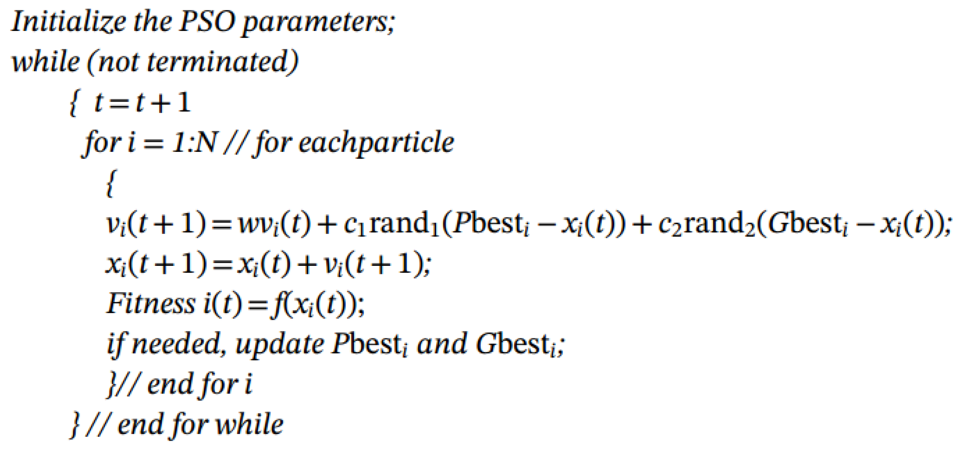
Figure 3.
Algorithm for biogeography based optimization (BBO).
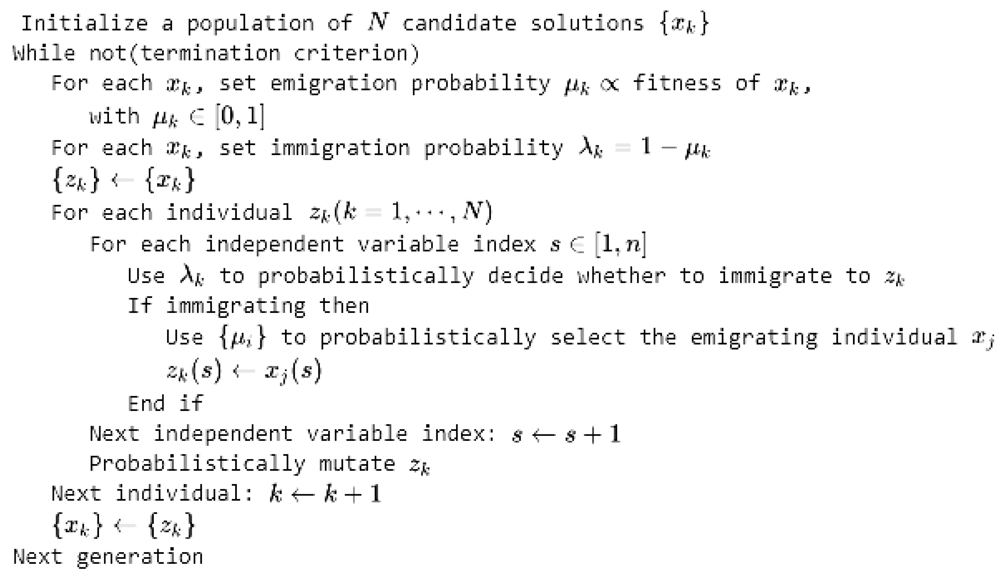
Figure 4.
3D contour plots or surfaces showing relationship between different input and output process parameters (a) MRR with Gap Voltage and Pulse Current; (b) MRR with Pulse-on-time and Pulse-off-time; (c) Ra with Gap Voltage and Pulse Current;and (d) Ra with Pulse-on-time and Pulse-off-time.
Figure 4.
3D contour plots or surfaces showing relationship between different input and output process parameters (a) MRR with Gap Voltage and Pulse Current; (b) MRR with Pulse-on-time and Pulse-off-time; (c) Ra with Gap Voltage and Pulse Current;and (d) Ra with Pulse-on-time and Pulse-off-time.
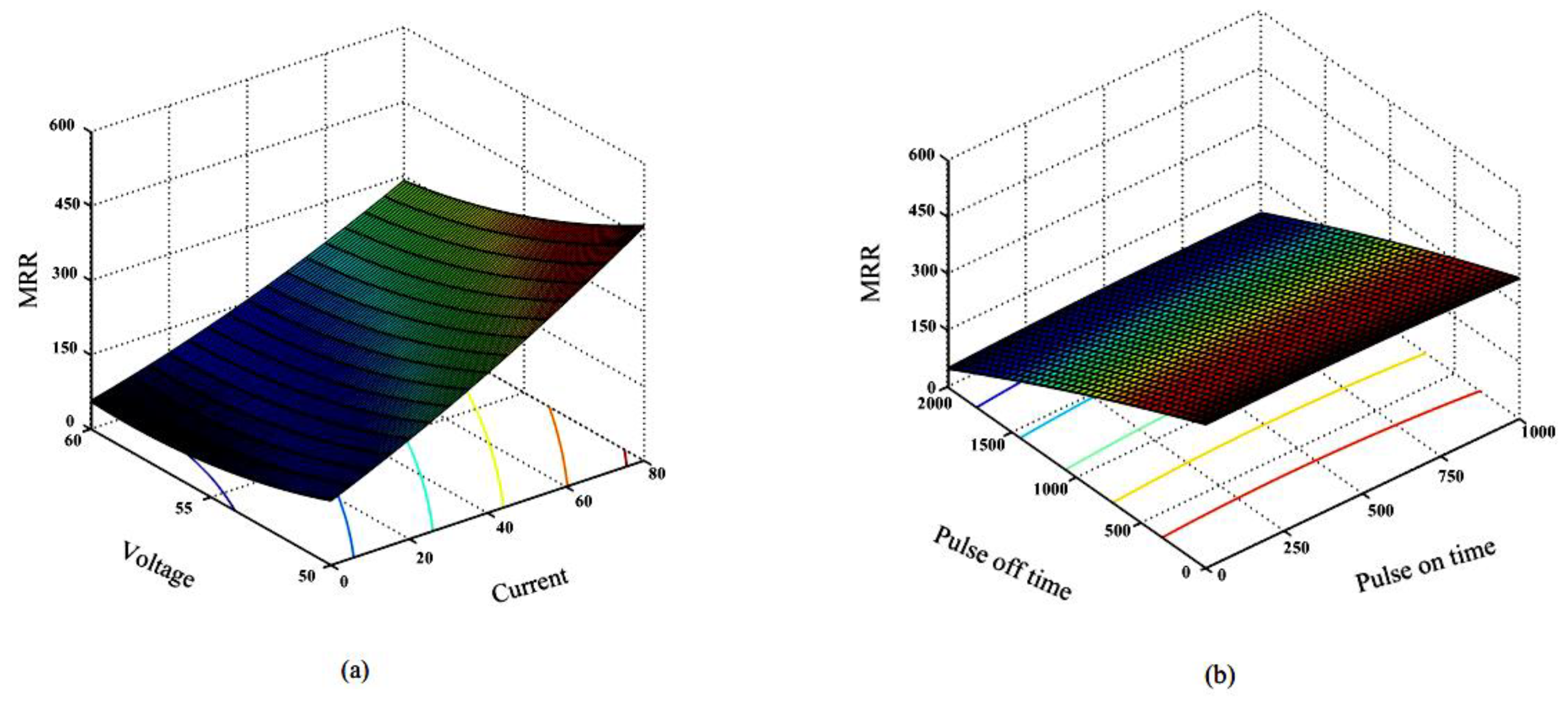
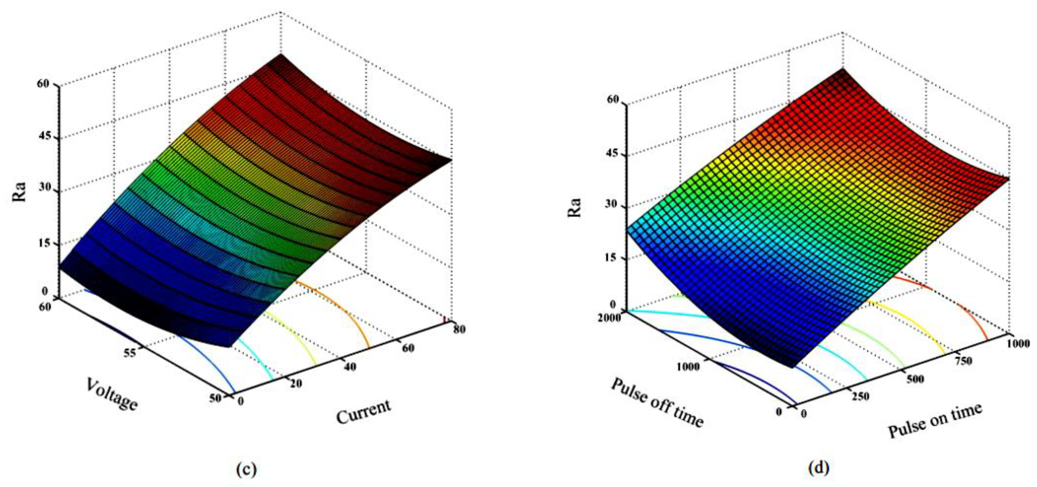
Figure 5.
Effects of input parameters on output parameters.
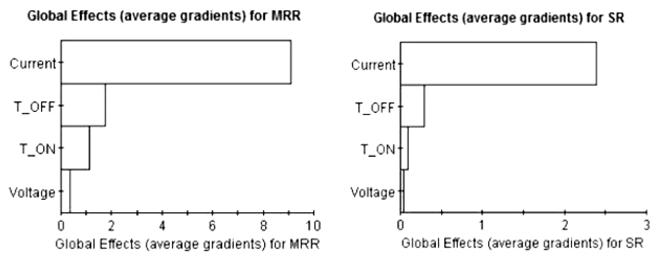
Figure 6.
SEM images: (a) before machining; (b) after machining with initial parameters; (c) after machining with optimal parameters computed using BBO; and (d) after machining with optimal parameters computed using PSO.
Figure 6.
SEM images: (a) before machining; (b) after machining with initial parameters; (c) after machining with optimal parameters computed using BBO; and (d) after machining with optimal parameters computed using PSO.

Figure 7.
Convergence plot for BBO and PSO algorithm.
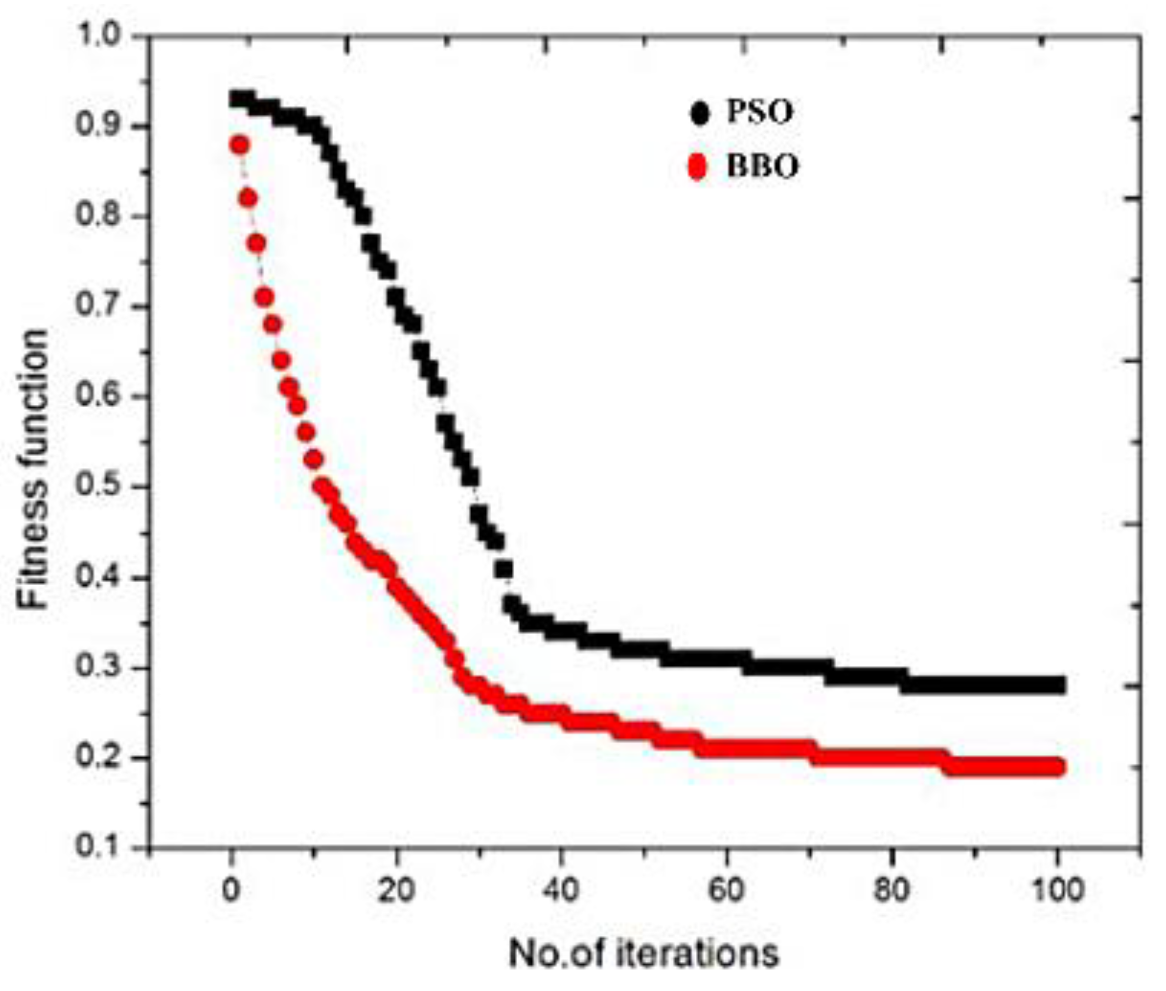
Figure 8.
Computational time for BBO and PSO algorithms.

Table 1.
Chemical composition of EN 31 Tool Steel.
| Elements | C | Mn | Si | P | S | Cr | Fe |
|---|---|---|---|---|---|---|---|
| Chemical Composition (wt. %) | 1.07 | 0.58 | 0.32 | 0.04 | 0.03 | 1.12 | 96.84 |
Table 2.
Mechanical properties of EN 31 Tool Steel.
| Thermal Conductivity (w/mk) | 46.6 |
| Density (gm/cc) | 7.81 |
| Electrical Resistivity (ohm-cm) | 0.0000218 |
| Specific heat capacity (j/gm-°C) | 0.475 |
Table 3.
Mechanical properties of electrode.
| Copper (99% Pure) | |
|---|---|
| Thermal Conductivity (w/mk) | 391 |
| Density (gm/cc) | 1083 |
| Electrical Resistivity (ohm-cm) | 1.69 |
| Specific heat capacity (j/gm-°C) | 0.385 |
Table 4.
Specification of Die-Sinking electrical discharge machining (EDM) Machine.
| Machining Conditions | |
|---|---|
| Machine Used | CNC EDM (EMT 43) (Electronica) |
| Electrode | Polarity Positive |
| Dielectric | EDM Oil |
| Work piece | Oil Hardened Non Shrinking Steel (48–50 HRC) |
| Electrode | Electrolytic Copper (99.9% Purity) |
| Flushing Condition | Pressure Flushing through 6 mm hole through work piece |
Table 5.
Experimental observation for material removal rate (MRR) and roughness parameter (Ra).
| S. No. | IP (A) [A] | Ton (µs) [B] | Toff (µs) [C] | V (V) [D] | MRR mm3/min | (Ra) (µm) | S. No. | IP (A) [A] | Ton (µs) [B] | Toff (µs) [C] | V (V) [D] | MRR mm3/min | (Ra) (µm) |
|---|---|---|---|---|---|---|---|---|---|---|---|---|---|
| 1 | 1 | 5 | 11 | 60 | 1.2 | 1.97 | 26 | 6 | 200 | 425 | 50 | 25.0 | 10 |
| 2 | 1 | 10 | 22 | 55 | 2.5 | 2.4 | 27 | 10 | 50 | 107 | 50 | 50.0 | 10 |
| 3 | 1 | 20 | 43 | 55 | 2.1 | 3.1 | 28 | 10 | 75 | 160 | 50 | 48.0 | 10 |
| 4 | 1 | 30 | 64 | 55 | 2.3 | 2.7 | 29 | 10 | 100 | 213 | 50 | 60.0 | 11.6 |
| 5 | 1 | 50 | 107 | 55 | 3.1 | 2.9 | 30 | 10 | 150 | 319 | 50 | 58.0 | 13.1 |
| 6 | 1.5 | 5 | 11 | 60 | 2.0 | 2.4 | 31 | 10 | 200 | 425 | 50 | 56.0 | 14.4 |
| 7 | 1.5 | 10 | 22 | 55 | 4.9 | 3.0 | 32 | 20 | 100 | 213 | 50 | 133.0 | 15 |
| 8 | 1.5 | 20 | 43 | 55 | 4.7 | 3.1 | 33 | 20 | 150 | 319 | 50 | 121.0 | 16.8 |
| 9 | 1.5 | 50 | 107 | 55 | 6.2 | 3.1 | 34 | 20 | 200 | 425 | 50 | 132.0 | 18.0 |
| 10 | 1.5 | 100 | 213 | 55 | 4.0 | 3.3 | 35 | 20 | 500 | 1063 | 50 | 124.0 | 23.7 |
| 11 | 2 | 5 | 11 | 60 | 2.3 | 2.6 | 36 | 30 | 150 | 319 | 50 | 182.0 | 18.8 |
| 12 | 2 | 10 | 22 | 55 | 7 | 2.6 | 37 | 30 | 200 | 425 | 50 | 174.0 | 20.5 |
| 13 | 2 | 20 | 43 | 55 | 8 | 3 | 38 | 30 | 500 | 1063 | 50 | 187.0 | 27.4 |
| 14 | 2 | 50 | 107 | 55 | 9 | 3.6 | 39 | 30 | 1000 | 2125 | 50 | 158.0 | 34.2 |
| 15 | 3 | 5 | 11 | 50 | 7.8 | 2.2 | 40 | 40 | 100 | 213 | 50 | 244.0 | 18 |
| 16 | 3 | 10 | 22 | 50 | 11.5 | 2.7 | 41 | 40 | 150 | 319 | 50 | 240.0 | 20.4 |
| 17 | 3 | 20 | 43 | 50 | 12.6 | 3.7 | 42 | 40 | 200 | 425 | 50 | 218.0 | 22.3 |
| 18 | 3 | 50 | 107 | 50 | 13.7 | 4.9 | 43 | 40 | 500 | 1063 | 50 | 270.0 | 29.6 |
| 19 | 3 | 100 | 213 | 50 | 10.3 | 6 | 44 | 40 | 1000 | 2125 | 50 | 216.0 | 36.5 |
| 20 | 6 | 5 | 11 | 50 | 17.0 | 2.8 | 45 | 40 | 2000 | 4250 | 50 | 240.0 | 45 |
| 21 | 6 | 10 | 22 | 50 | 26.0 | 3.6 | 46 | 50 | 200 | 425 | 50 | 330.0 | 25 |
| 22 | 6 | 20 | 43 | 50 | 29.0 | 4.5 | 47 | 50 | 400 | 850 | 50 | 350.0 | 32 |
| 23 | 6 | 50 | 107 | 50 | 31.0 | 6.3 | 48 | 50 | 500 | 1063 | 50 | 310.0 | 32 |
| 24 | 6 | 100 | 213 | 50 | 32.0 | 7.7 | 49 | 50 | 1000 | 2125 | 50 | 310.0 | 41 |
| 25 | 6 | 150 | 319 | 50 | 28.0 | 8.7 | 50 | 50 | 2000 | 4250 | 50 | 300.0 | 50 |
Table 6.
Initial Population and Fitness Value.
| Particle | A | B | C | D | MRR | Ra | Fitness Value |
|---|---|---|---|---|---|---|---|
| 1 | 30 | 500 | 1063 | 50 | 187 | 27.4 | 0.6814 |
| 2 | 40 | 1000 | 2125 | 55 | 216 | 36.5 | 0.5038 |
| 3 | 50 | 2000 | 4250 | 60 | 300 | 50 | 0.5672 |
Table 7.
Changed position of particles after the first iteration.
| Particle | A | B | C | D |
|---|---|---|---|---|
| 1 | 2.92 | 60 | 75 | 5.5 |
| 2 | 2.4 | 30 | 35 | −4.5 |
| 3 | 0.5 | 0.5 | 0.5 | 0.05 |
Table 8.
New position of particles after the first iteration.
| Particle | A | B | C | D | MRR | Ra | Fitness Value |
|---|---|---|---|---|---|---|---|
| 1 | 32.92 | 560 | 1138 | 55.50 | 184.25 | 26.50 | 0.768 |
| 2 | 42.40 | 1030 | 2160 | 50.50 | 216.35 | 34.50 | 0.659 |
| 3 | 50.50 | 2000.50 | 4250.5 | 60.05 | 302.30 | 48.75 | 0.724 |
Table 9.
Validation test for EDM through PSO.
| I | Ton | Toff | V | MRR | Ra | ||||
|---|---|---|---|---|---|---|---|---|---|
| 40 | 110 | 230 | 50 | Experimental | Optimized | %Error | Experimental | Optimized | %Error |
| 238 | 235 | 1.26 | 18.4 | 18.1 | 1.63 | ||||
Table 10.
Validation test for EDM through BBO.
| I | Ton | Toff | V | MRR | Ra | ||||
|---|---|---|---|---|---|---|---|---|---|
| 40 | 100 | 210 | 50 | Experimental | Optimized | %Error | Experimental | Optimized | %Error |
| 240 | 242 | 0.83 | 18.01 | 17.98 | 0.166 | ||||
© 2018 by the authors. Licensee MDPI, Basel, Switzerland. This article is an open access article distributed under the terms and conditions of the Creative Commons Attribution (CC BY) license (http://creativecommons.org/licenses/by/4.0/).
Share and Cite
MDPI and ACS Style
Faisal, N.; Kumar, K. Optimization of Machine Process Parameters in EDM for EN 31 Using Evolutionary Optimization Techniques. Technologies 2018, 6, 54. https://doi.org/10.3390/technologies6020054
AMA Style
Faisal N, Kumar K. Optimization of Machine Process Parameters in EDM for EN 31 Using Evolutionary Optimization Techniques. Technologies. 2018; 6(2):54. https://doi.org/10.3390/technologies6020054
Chicago/Turabian StyleFaisal, Nadeem, and Kaushik Kumar. 2018. "Optimization of Machine Process Parameters in EDM for EN 31 Using Evolutionary Optimization Techniques" Technologies 6, no. 2: 54. https://doi.org/10.3390/technologies6020054
Note that from the first issue of 2016, this journal uses article numbers instead of page numbers. See further details here.