1. Introduction
Pervasive sensing technology has the potential to enhance information gathering and processing in diverse applications. A typical wireless sensor network (WSN) employs multiple sensors, each equipped with devices capable of sensing, processing, and communication [
1,
2,
3,
4]. The advantages of WSNs include flexibility in deployment and scalability, low cost and fast initial set-up. Recent advances in micro-sensors have enabled WSN to a wide range of applications, such as battlefield surveillance, environmental monitoring, and health care applications [
5,
6,
7,
8]. Significant challenges exist and need to be addressed in order for the envisaged application to become a reality. For instance, the individual sensors are incredibly resource constrained. They have limited storage capacity and communication bandwidth. In addition, in many WSN applications, sensors operate on irreplaceable power supply, making it necessary to conserve power for prolonged lifetime. From an energy-consumption perspective, transmitting or receiving one kilobyte of information is equivalent to computing 3 million of instructions [
9], so it is recommended to make a computation at the sensor level instead of transmitting whenever it is possible.
Decisions fusion represents a formal framework that deals with data collected from different resources to obtain a greater quality of global decision about a certain phenomena. Decisions fusion with uncertainty has been investigated and a Bayesian sampling approach has been proposed to address this issue [
10]. In [
11,
12], the optimum fusion rule has been obtained under the conditional independence assumption. A fusion of decisions that are correlated to each other has been studied in [
13]. Distributed detection in a constrained system has been considered in [
14]. Decisions fusion in WSN operated with a multiple input multiple output (MIMO) channel has been investigated in [
15,
16]. Universal decentralized detection in a bandwidth-constrained sensor network with binary decisions made by sensor nodes has been constructed in [
17]. Universal detectors for the decision fusion problem have also been considered in [
18].
The distributed detection problem in WSNs has been studied using two kinds of communication channels: the traditional parallel access channel (PAC) in which each sensor has a dedicated independent channel to fusion center (FC) and the multiple access channel (MAC) in which the FC receives a coherent superposition of the sensor transmissions [
19,
20]. On the one hand, for networks with a large number of sensors, PAC implies a large bandwidth requirement and a large detection delay. On the other hand, the bandwidth requirement of MAC does not depend on the number of sensors, but due to the additive nature of the channel, the received signal at the FC is usually not sufficient for reliable detection.
Channel-aware distributed detection has been proposed in [
21,
22], which integrates the wireless channel conditions in algorithm design. Channel-aware distributed detection has also been considered for a decode-then-fuse model and parallel access channels in [
23], as well as for a MIMO channel model with both instantaneous and statistical channel state information (CSI) in [
24,
25,
26]. The fusion of decisions transmitted over Rician fading channels has been investigated in [
27]. In [
28], five different fusion rules have been investigated in a three-layer parallel access WSN fusion model over Rayleigh fading channels. These fusion rules are the likelihood ratio test (LRT), equal gain combiner (EGC), maximum ratio combiner (MRC), Chair–Varshney and the likelihood ratio test based on channel statistics (LRT-CS). It is shown in [
28] that the LRT fusion rule is the optimum fusion rule. Nevertheless, the LRT requires the CSI which should be estimated. In addition, the local sensors’ performance indices must be transmitted by each sensor to the FC. Thus, applying LRT at the FC is too costly since WSNs are known to be a constrained system in terms of communication bandwidth and energy consumption. On the other hand, the EGC is a simple fusion rule since it does not require any knowledge about the channel or the local sensors’ performance indices. Optimal local sensor detection does not necessarily yield a global optimal detection and compromises should be made with each other as well as the fusion rule at the FC.
Taking into account the limitation on energy and bandwidth of WSNs, we propose in this paper a modification to the existing three-layer PAC decision fusion model for WSNs where the LRT is applied locally to each sensor. Applying the LRT at the sensors level does not require the CSI or transmitting local sensors’ performance indices from each sensor to the FC. It only requires the instantaneous channel signal-to-noise ratio (SNR). Moreover, we propose to apply selection combining (SC) as decision fusion method at the FC.
The remainder of the paper is organized as follows.
Section 2 presents the existing three-layer WSN system model and the state-of-the-art decision fusion rules.
Section 3 introduces the proposed WSN system model. In
Section 4, a comparative simulation study is carried out between the proposed WSN model and the existing WSN model. Conclusions are drawn in
Section 5.
2. Traditional Three-Layer WSN System Model
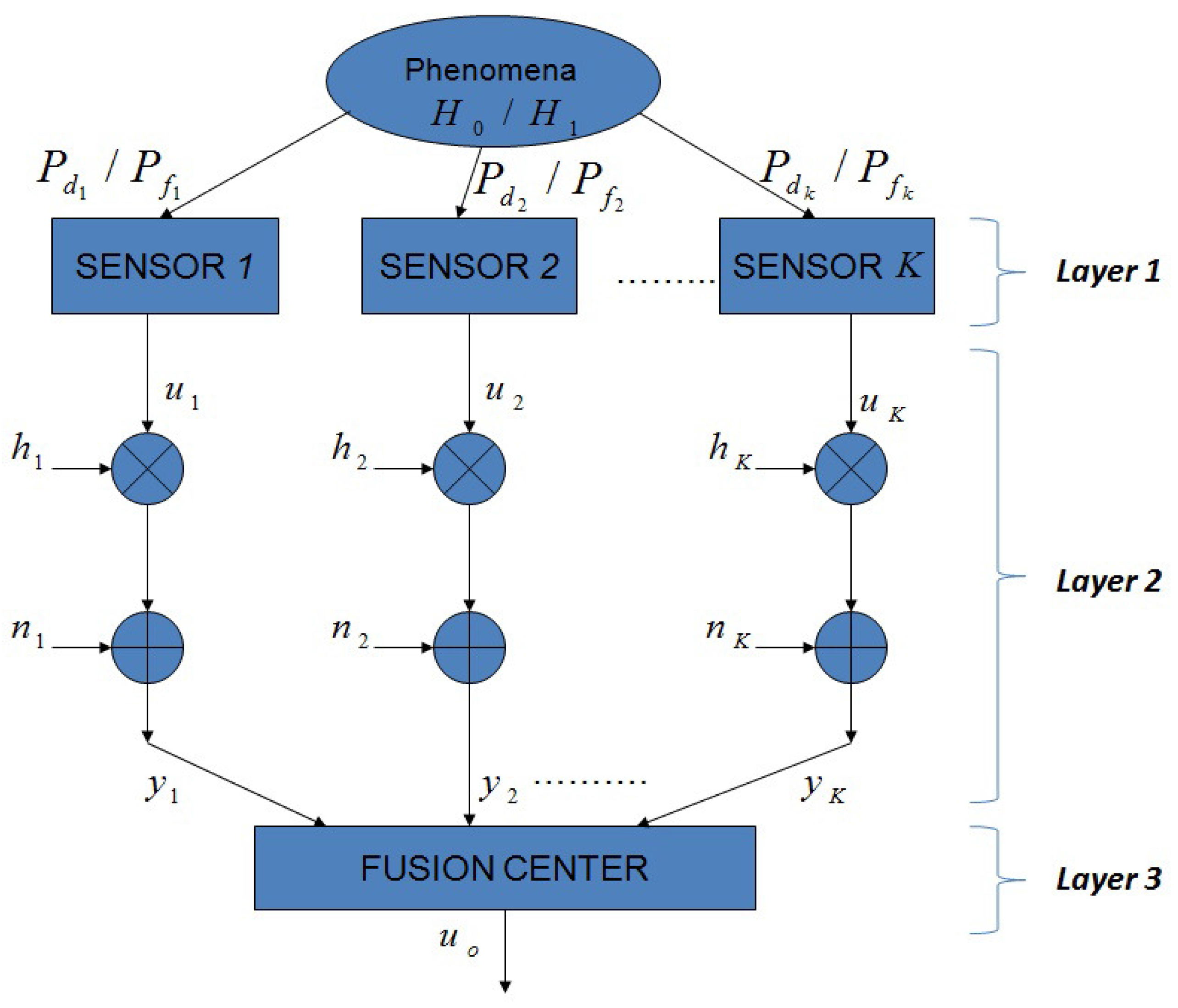
The traditional three-layer PAC decision fusion model for WSNs in the presence of additive white Gaussian noise (AWGN) and fading channels is illustrated in
Figure 1. There are two hypotheses under testing,
(target present), and
(target absent). Each sensor receives noisy measurements and processes these measurements in order to make decisions regarding the hypothesis under testing. Then, each sensor transmits the obtained binary decision to the FC through parallel access channels which undergo AWGN and Rayleigh fading.
For WSNs with limited resources, the effect due to channel fading and noise renders the information received at the FC not completely reliable. Corruption on the received local decisions will lead to performance loss if they are not properly considered. The traditional three-layer parallel WSN system model can be described in detail as follows.
2.1. Layer 1: Sensors
In this layer, all of the local sensors receive noisy measurements regarding a specific hypothesis. In this work, we assume that the observations are conditionally independent of each other. After receiving its observation,
, each sensor,
k, makes a hard (binary) decision:
is sent if
is decided, and
is sent otherwise, where
and
K is the total number of sensors in the network. The hard binary decision can be formalized as follows:
In addition, we assume that each sensor makes a binary decision based on its own observation. The detection performance of each local sensor node can be characterized by its corresponding probability of detection and probability of false alarm, denoted by
and
, respectively, for the
kth sensor:
In general, these pairs may not be identical and they are functions of SNRs as well as the detection threshold at each sensor.
2.2. Layer 2: Fading and Noisy Channels
Decisions at local sensors, denoted by
for
are transmitted over parallel channels that are assumed to undergo independent fading. Since most of the WSNs operate at short range and low bit rate due to power and energy limitations, the fading channels are assumed to be flat. We further assume phase coherent reception, thus the effect of a fading channel is further simplified as a real scalar multiplication given that the transmitted signal is assumed to be binary. The statistics of the real scalar, denoted by
, is determined by the fading type. For example, for homogeneous scattering background, Rayleigh distribution best describes the envelope of a fading signal. In the development of fusion rules, the gain of the fading channel is considered as an unknown constant during the transmission of a single local decision. We assume that the channel noise is AWGN and uncorrelated from channel to channel. Thus, the input to the FC for the
kth sensor is given by
where
is Rayleigh distributed fading channel gain with unit power (i.e.,
) and
is a zero-mean Gaussian random variable with variance
.
2.3. Layer 3: Fusion Center
The FC is the most important part in the WSN system which makes a global decision
regarding a certain phenomena based on the received
data for all
k. This is done by making use of a certain fusion rule applied at the FC. According to the used fusion rule at the FC, some other parameters may be required in order to make the global decision such as the CSI and the local sensors’ performance indices. The function of the FC after forming a certain statistic Λ can be expressed as:
where
T is the decision threshold at the FC.
To facilitate our comparisons later, we give a brief review here of the fusion rules developed in [
22,
28]. Namely, the likelihood ratio test (LRT), equal gain combiner (EGC), maximum ratio combiner (MRC), Chair–Varshney and the likelihood ratio test based on channel statistics (LRT-CS). In addition, the so-called selection combining will also be investigated as a fusion rule.
2.3.1. The Optimal LRT
By assuming instantaneous channel state knowledge regarding the fading channel and the local sensor performance indices, i.e., the
and
values, the optimal LRT-based fusion rule has been derived in [
22], with the fusion statistic Λ given by
The LRT value is then compared with a threshold at the FC to make a final decision. While the form of the LRT based fusion statistic is straightforward to implement, it does need both the local sensor performance indices and complete channel knowledge.
2.3.2. Chair–Varshney Fusion Rule
In [
28], the following statistic, termed as the Chair–Varshney fusion statistic, has been shown to be a high-SNR approximation to Λ
does not require any knowledge regarding the channel gain but does require and for all k. This approach, however, suffers significant performance loss at low channel SNR.
2.3.3. MRC Fusion Rule
It has been shown in [
28] that, for small values of channel SNR, Λ in Equation (
5) reduces to
Furthermore, if the local sensors are identical, i.e.,
and
for all
ks, then Λ further reduces to a form analogous to a MRC statistic
in Equation (
8) does not require the knowledge of
and
provide
. Knowledge of the channel gain is, however, required.
2.3.4. EGC Fusion Rule
Motivated by the fact that resembles a MRC statistic for diversity combining, a third alternative in the form of an EGC has been proposed in [
28], which requires a minimum amount of information:
Interestingly enough, this simple alternative fusion rule outperforms both MRC and Chair–Varshney fusion rules for a wide range of SNR in terms of its detection performance [
28].
2.3.5. LRT-CS Fusion Rule
A fusion rule based on the optimal LRT has been proposed in [
28]. This fusion rule requires the knowledge about the wireless channel statistical characteristics instead of the instantaneous CSI. This fusion rule is given by
where
and
is the complementary distribution function of the standard Gaussian.
The above fusion rule outperforms both the EGC and Chair–Varshney fusion rules and has better performance than the MRC fusion rule for most practical SNR values (except for very low SNR values) [
28].
2.3.6. SC Fusion Rule
The selection combining (SC) fusion rule has lower implementation complexity compared to the MRC and the EGC, and it is based on selecting the branch that has the maximun instantaneous channel SNR as follows:
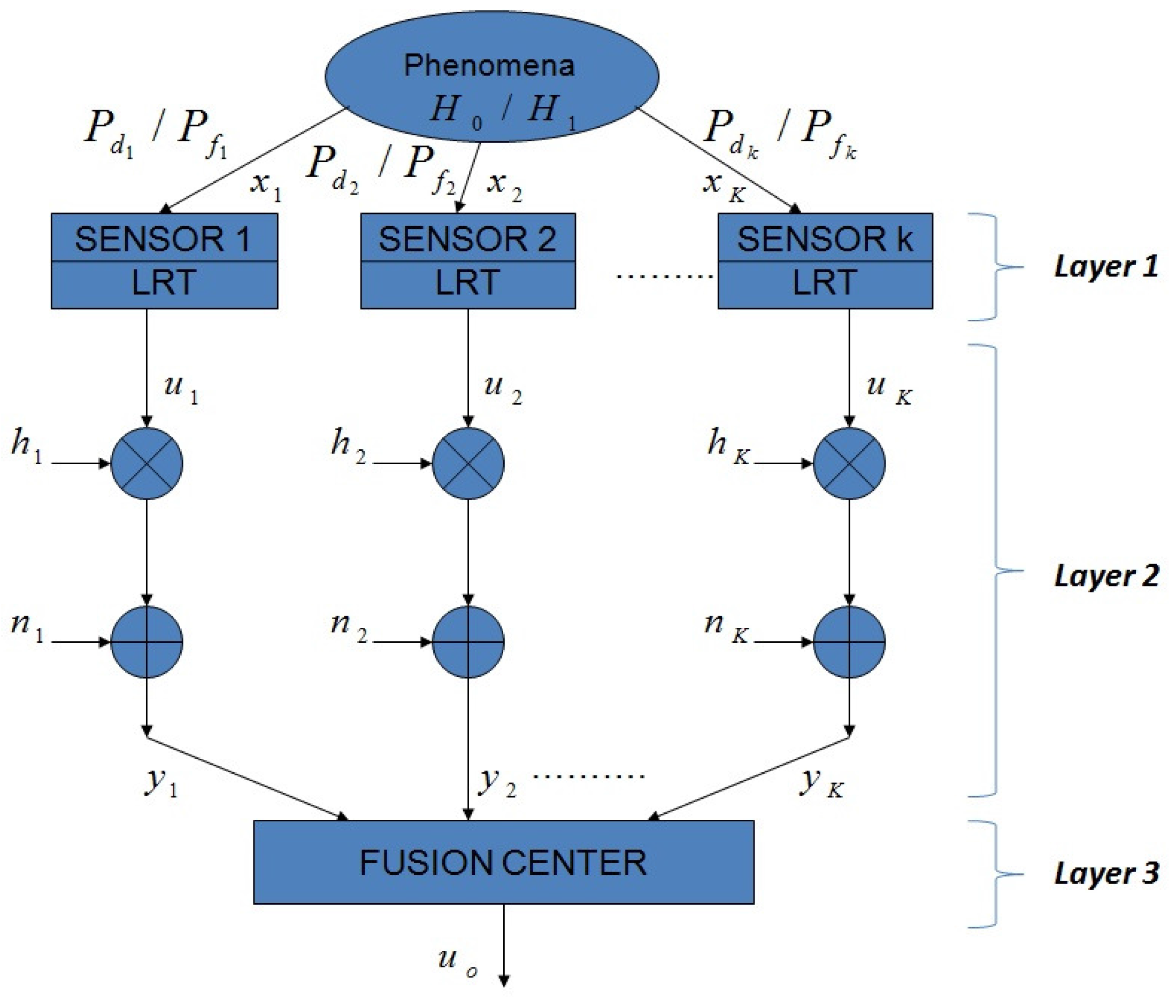
3. Proposed Three-Layer WSN System Model
In this section, we propose a modification to the traditional three-layer WSN system model by applying the optimal LRT as a local decision making method at the sensors level as shown in
Figure 2. Applying the LRT at the sensors level does not require the CSI or transmitting the local sensors performance indices, i.e.,
and
for all
ks. Indeed, from the energy consumption perspective, transmitting or receiving one kilobyte of information is equivalent to computing 3 million instructions [
9], so it is recommended to make a computation in the sensor level instead of transmitting whenever it is possible.
Assuming that there are two hypothesis under test (
and
), the measured noisy signal at each sensor can be described by the following equation:
where
represents the
signal in the case of
and
is the corresponding sensor measurement additive white noise which is not necessarily Gaussian and whose variance is
. Note that the sensor measurement noise
is different from the channel noise
. In this work, we assume that the absence or the presence of the signal under interest
, i.e.,
or
, respectively, is described by either 1 or 0 as follows:
Then, the LRT based decision for each sensor can be written as
where
T is the decision threshold. In the special case when the sensor measurement noise is assumed to be Gaussian, the measured information
follows the normal distribution with zero-mean and variance of
in the case of
, and unit-mean with variance of
in the case
as described by
Assuming independent identically distributed (i.i.d) measurements among the sensors, the required probability density functions (PDFs) can be expressed as
Substituting Equation (
16) into Equation (
14) yields to the LRT statistics
at sensor level
It can be noticed from Equation (
17) that applying the LRT at the sensors level requires no prior information regarding the channel and no information about local sensors performance indices. It only requires the instantaneous channel SNR.
Now, each sensor makes a local decision regarding the absence or the presence of a certain hypothesis,
and
, respectively, according to
It should be noted that, due to the sensor measurement noise Gaussian assumption, the traditional model in
Figure 1 and the proposed model in
Figure 2 are statistically equivalent if a varying threshold is considered at Equation (
1). Nevertheless, in the following, the proposed model leads to improved performance by introducing an optimized local sensor threshold.
The performance of the LRT is mainly characterized by the probability of correctly recognizing the presence of the signal while it is actually present (probability of detection) and the probability of wrongly recognizing the signal as present while it is actually absent (probability of false alarm). The probability of a false alarm is defined as
Equation (
19) is the integral of a Gaussian PDF, so it can be solved by using the definition of the error function
[
29], as follows:
changing the variables
, Equation (
19) can be rewritten as
Finally, Equation (
21) can be solved to obtain the threshold
T in term of the inverse error function (
) as follows:
The probability of detection for the LRT is defined as follows:
Again, applying the definition of the error function in Equation (
20) leads to
Substituting Equation (
22) in Equation (
24) and make use of the complementary error function
in order to eliminate the threshold
T leads to
Equation (
25) describes the performance of the LRT in terms of fixed channel signal-to-noise ratio
and fixed probability of false alarm
.
4. Simulation Results
In this section, the relative performance of different fusion rules applied at the FC in the proposed WSN system model is examined. In addition, a performance comparison between the traditional and the proposed WSN system model is carried out through simulation in order to obtain the receiver operating characteristics (ROC) curves for different fusion rules. Moreover, we studied the effect of various factors that may affect the performance of the FC such as the communication channel signal-to-noise ratio (SNR), total number of sensors in the network (i.e., K) and the local sensors’ performance indices (i.e., and ).
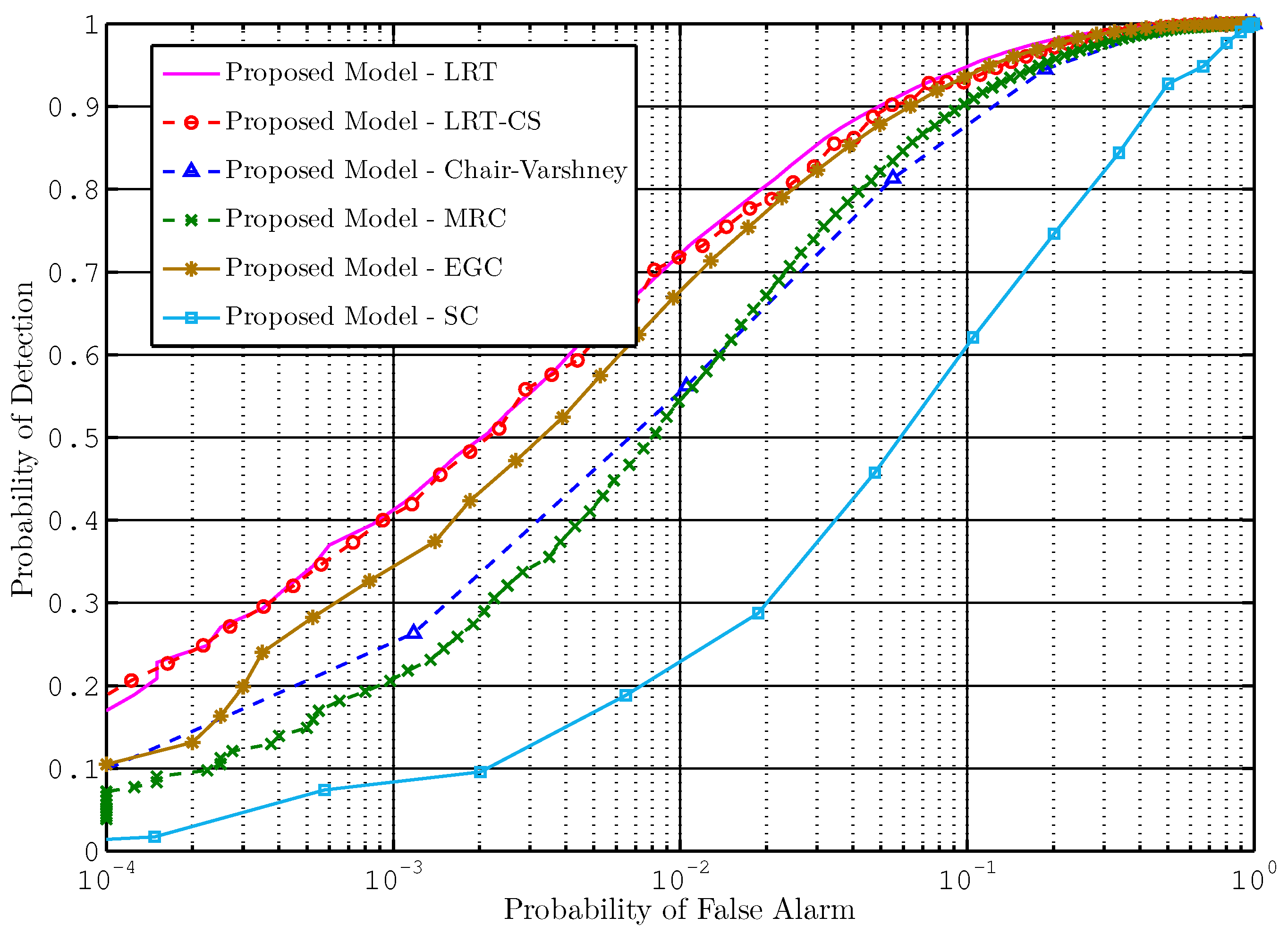
In the first simulation scenario, ROC performance comparison among the various fusion rules applied at the proposed WSN system model is carried out. We assume that all sensors receive noisy measurements and all have the same SNR and thus having the same performance indices. Moreover, the channels between the sensors and the FC all have the same SNR. ROC curves for different fusion rules applied at the proposed WSN system model and channel SNR of 5 dB are plotted in
Figure 3. The local sensors’ performance indices
and
are assumed to be 0.5 and 0.05, respectively. The total number of sensors in the network is fixed at
. According to
Figure 3, the LRT and the LRT-CS fusion rules have the best performance, whereas the SC fusion rule has the worst performance.
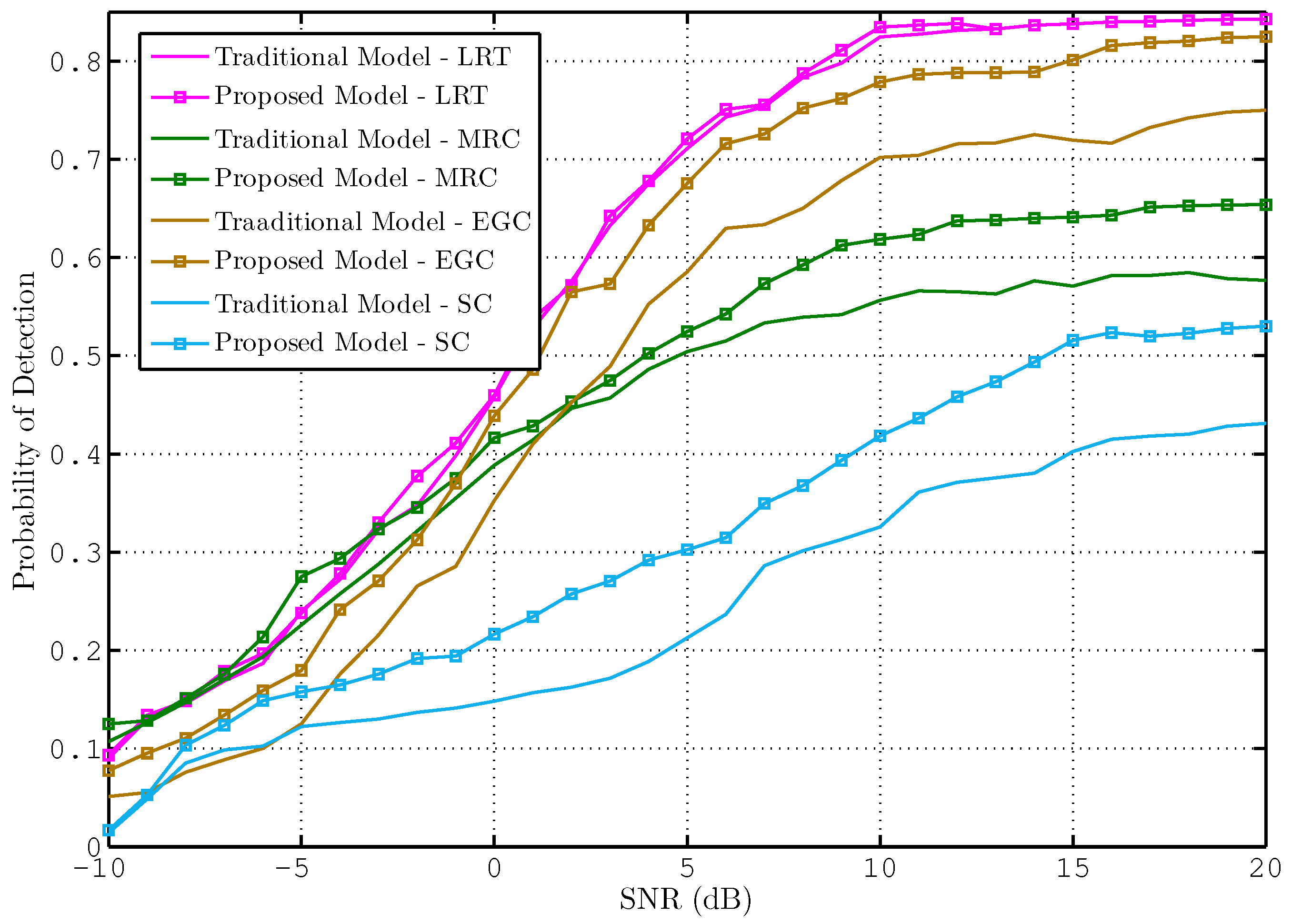
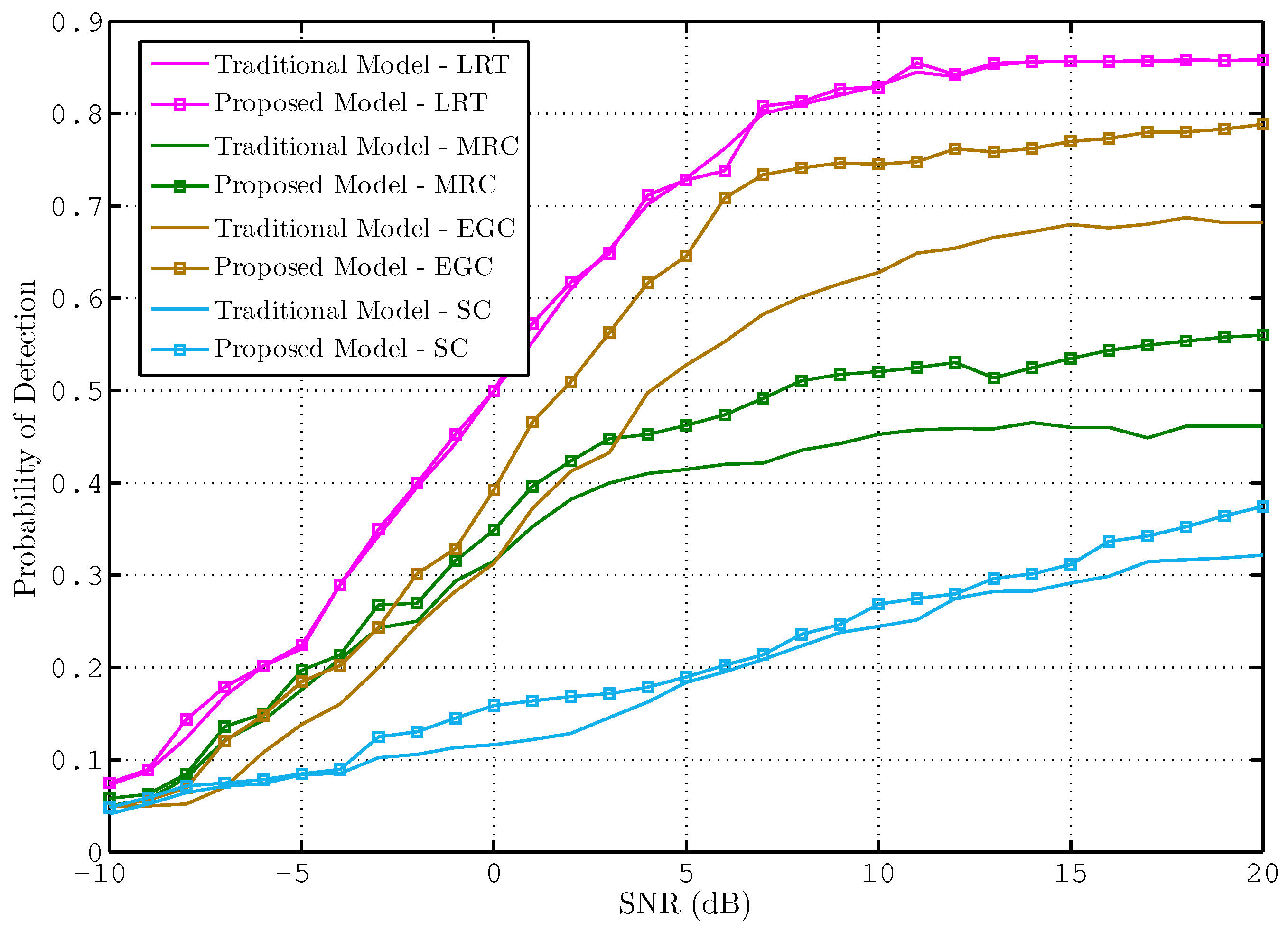
In the second simulation scenario, a comparison is made between the traditional and the proposed WSN model with the various fusion rules for variable channel SNR. We assume that the local sensors performance indices are identical and also the channels’ SNR between the sensors and the FC are identical. From
Figure 4, one can notice that the performance of the proposed model is better than that of the traditional model for the various fusion rules and for a wide range of channel SNR. While the LRT shows the best performance among the other fusion rules in both models, the EGC fusion rule applied at the proposed model provides a performance very similar to that of LRT-CS for a wide range of SNRs and better performance than other fusion rules such as MRC and Chair–Varshney fusion rules. Thus, applying the LRT at the sensors level and EGC at the FC can significantly raise the performance of the proposed model when compared to the traditional model. Moreover,
Figure 4 shows that the proposed model could significantly increase the performance of MRC and SC fusion rules for high channel SNR.
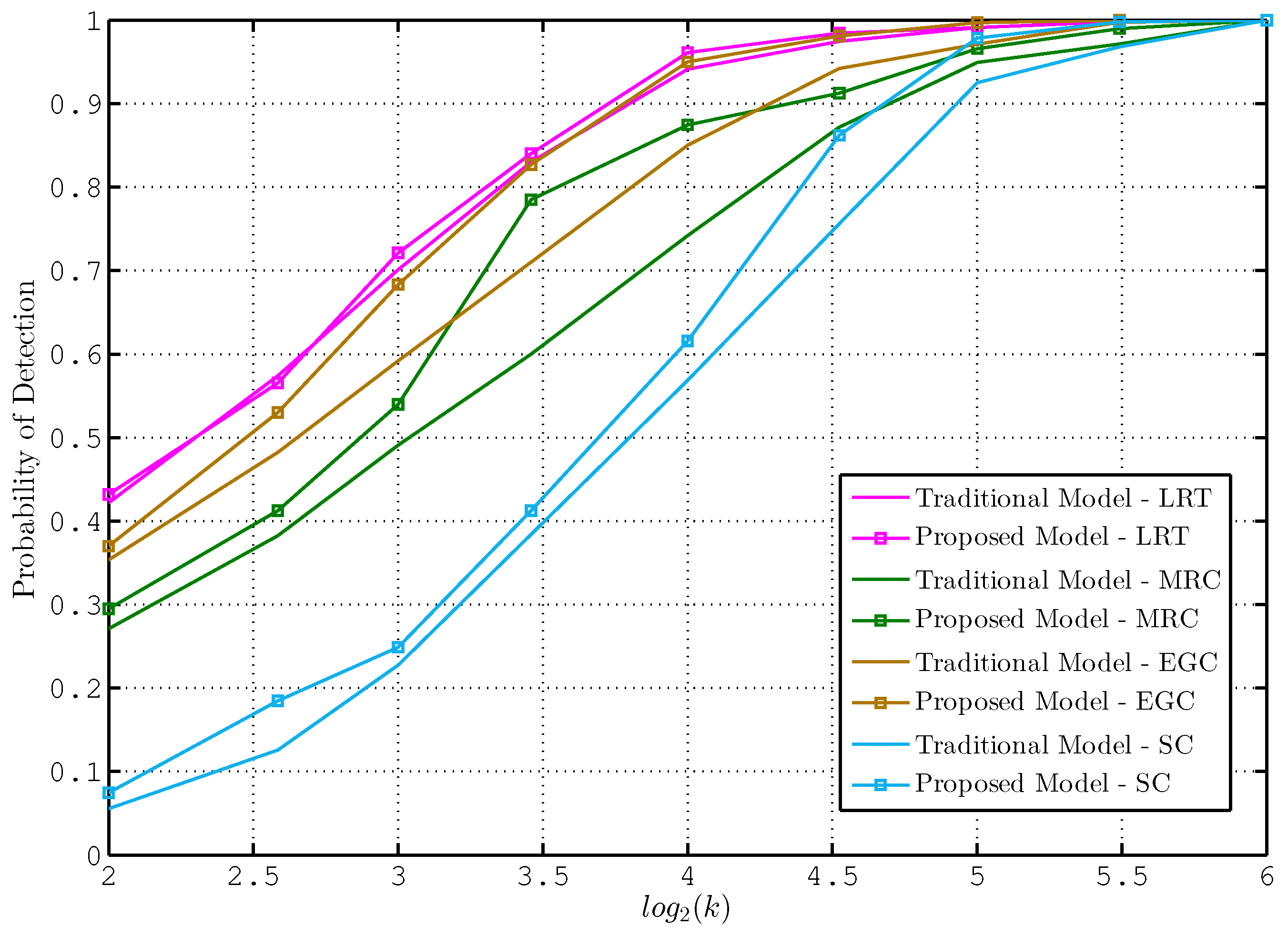
In the third simulation experiment, we investigate the effect of number of sensors
K on the traditional and proposed model for the various fusion rules. We assume that the average channel SNR is fixed to 5 dB, the local sensors have performance indices of
,
, and these indices are identical among all sensors. It can be observed from
Figure 5 that the proposed model outperforms the traditional model for the various fusion rules and for different number of sensors
. In addition, one can notice that, even for small number of sensors
K, the performance of the EGC applied at the proposed model is nearly the same to that of the optimum LRT and outperforms all other fusion rules and shows more robustness regarding the total number of sensors.
In the fourth simulation scenario, the effect of non-identical sensor performance indices is investigated. We assume that all sensors have the same probability of false alarm (
) and a different probabilities of detection, where
and
. From
Figure 6, the EGC fusion rule applied at the proposed model provides a relatively good performance when compared to SC and MRC and is similar to that of the LRT. Thus, the EGC fusion rule applied to the proposed WSN model could be a good alternative for the optimum LRT fusion rule applied at the FC.
5. Conclusions
In this paper, we propose an improved decision fusion model for WSNs over Rayleigh fading channels where the LRT is applied locally to each sensor. The application of the LRT at the sensors level improves the local decision and does not require either CSI or the transmission of local sensor performance indices from sensors to FC. This is essential for energy and bandwidth constrained WSNs. The improved local decision at each sensor enhanced the performance of different fusion rules when applied at the FC.
According to the comparative simulation study we that we carried out, the proposed WSN model outperforms the traditional one for all fusion rules considered and for a wide range of SNR. In addition, applying the EGC fusion rule at the FC of the proposed WSN model could be considered as a good alternative for the optimum LRT fusion rule as it provides a comparable performance to that of the LRT fusion rule and better performance than other fusion rules. Therefore, it is recommended to use the LRT at the sensor level and the EGC fusion rule at the FC.

