
Fast and Efficient Entropy Coding Architectures for Massive Data Compression

Department of Information and Communications Engineering, Universitat Autònoma de Barcelona, 08193 Bellaterra, Spain
Technologies 2023, 11(5), 132; https://doi.org/10.3390/technologies11050132
Submission received: 19 July 2023
/
Revised: 22 September 2023
/
Accepted: 23 September 2023
/
Published: 26 September 2023
(This article belongs to the Special Issue Advances in Applications of Intelligently Mining Massive Data)
Abstract
:The compression of data is fundamental to alleviating the costs of transmitting and storing massive datasets employed in myriad fields of our society. Most compression systems employ an entropy coder in their coding pipeline to remove the redundancy of coded symbols. The entropy-coding stage needs to be efficient, to yield high compression ratios, and fast, to process large amounts of data rapidly. Despite their widespread use, entropy coders are commonly assessed for some particular scenario or coding system. This work provides a general framework to assess and optimize different entropy coders. First, the paper describes three main families of entropy coders, namely those based on variable-to-variable length codes (V2VLC), arithmetic coding (AC), and tabled asymmetric numeral systems (tANS). Then, a low-complexity architecture for the most representative coder(s) of each family is presented—more precisely, a general version of V2VLC, the MQ, M, and a fixed-length version of AC and two different implementations of tANS. These coders are evaluated under different coding conditions in terms of compression efficiency and computational throughput. The results obtained suggest that V2VLC and tANS achieve the highest compression ratios for most coding rates and that the AC coder that uses fixed-length codewords attains the highest throughput. The experimental evaluation discloses the advantages and shortcomings of each entropy-coding scheme, providing insights that may help to select this stage in forthcoming compression systems.
1. Introduction
Our society is immersed in a flow of data that supports all kinds of services and facilities such as online TV and radio, social networks, medical and remote sensing applications, or information systems, among others. The data employed in these applications are different, from text and audio to images and videos, strands of DNA, or environmental indicators, with a long etcetera. In many scenarios, these data are transmitted and/or stored for a fixed period of time or indefinitely. Despite enhancements on networks and storage devices, the amount of information globally generated increases so rapidly that only a small part can be saved [1,2]. Data compression is the solution to relieve Internet traffic congestion and the storage necessities of data centers.
The compression of information has been a field of study for more than a half-century. Since C. Shannon established the bases of information theory [3], the problem of how to reduce the number of bits to store an original message has been a relevant topic of study [4,5,6]. Depending on the data type and their purposes, the compression regime may be lossy or lossless. Image, video, and audio, for example, often use lossy regimes because the introduction of some distortion in the coding process does not disturb a human observer and achieves higher compression ratios [6]. Lossless regimes, on the other hand, recover the original message losslessly but achieve lower compression ratios. Also depending on the type and purpose of the data, the compression system may use different techniques. There are many systems specifically devised for particular types of data. Image and video compression capture samples that are transformed several times to reduce their visual redundancy [7,8,9,10]. Contrarily, compression of DNA often relies on a reference sequence to predict only the dissimilarities between the reference and the source [11]. There are universal methods like Lempel–Ziv–Welch [12,13] that code any kind of data, although they do not achieve the high compression ratios that specifically devised systems yield. In recent years, deep-learning techniques have been spread in many compression schemes to enhance transformation and prediction techniques, obtaining competitive results in many fields [14,15,16,17].
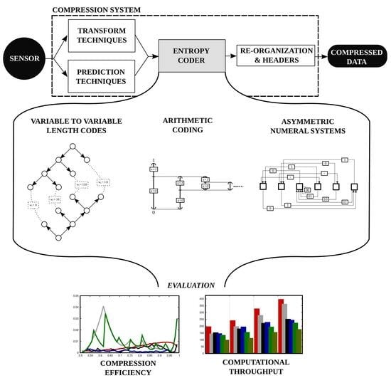
Regardless of the coding system and the regime employed, most compression schemes rely on a coding stage called entropy coding to reduce the amount of information needed to represent the original data. See in Figure 1 that this stage is commonly situated just after the transformation and/or prediction stages. These stages prepare the data for the entropy coder producing binary symbols x with a corresponding probability . In general, these symbols are (transformed to) binary, so is assumed in the following. The estimated or real [18,19] probability depends on the amount of redundancy found in the original data. Adjacent pixels in an image often have similar colors, for instance, so their binary representation can be predicted with a high probability. Both x and are fed to the entropy coder, which produces a compact representation of these symbols attaining compression. As Shannon’s theory of entropy dictates, the higher the probability of a symbol the lower its entropy, so higher compression ratios can be obtained. The main purpose of entropy coders is to attain coding efficiency close to the entropy of the original message while spending low computational resources, so large sets of data can be processed rapidly and efficiently.
Arguably, there are three main families of entropy coders. The first employs techniques that map one (or some) source symbols to codewords of different lengths. Such techniques exploit the repetitiveness of some symbols to represent them with a short codeword. The most complete theoretical model of such techniques is variable-to-variable length codes (V2VLC) [20,21]. The first entropy-coding technique proposed in the literature, namely Huffman coding [22], uses a similar technique that maps each symbol to a codeword of variable length. Other techniques similar to V2VLC are Golomb-Rice coding [23,24], Tunstall codes [25,26], or Khodak codes [27], among others [20,28], which have been adopted in many scenarios [29,30,31,32]. The second main family of entropy coders utilizes a technique called arithmetic coding (AC) [33]. The main idea is to divide a numeric interval into subintervals of varying sizes depending on the probability of the source symbols. The coding of any number within the latest interval commonly requires fewer bits than the original message and allows the decoder to reverse the procedure. Arithmetic coding has been widely spread and employed in many fields and standards [34,35,36,37] and there exist many variations and architectures [38,39,40,41,42,43]. The latest family of entropy coders is based on asymmetric numeral systems (ANS), which is a technique introduced in the last decade [44]. ANS divides the set of natural numbers into groups that have a size depending on the probability of the symbols. The coding of the original message then traverses these groups so that symbols with higher probabilities employ the groups of the largest size. The decoder reverses the path from the last to the first group, recovering the original symbols. There are different variants of ANS such as the range ANS or the uniform binary ANS, though the tabled ANS (tANS) is the most popular [45,46,47] since it can operate like a finite-state machine achieving high throughput. tANS has been recently adopted in many compression schemes [11,48,49], so it is employed in this work to represent this family of entropy coders.
The popularity of the aforementioned entropy-coding techniques has changed depending on the trends and necessities of applications. Since entropy coding is at the core of the compression scheme, efficiency, and speed are two important features. Before the introduction of ANS, Huffman coding and variants of V2VLC were generally considered the fastest techniques because they use direct mapping between source symbols and codewords. Nonetheless, they are not the most efficient in terms of compression [50]. Arithmetic coding was preferable in many fields due to its highest compression efficiency although it was criticized since it commonly requires some arithmetic operations to code each symbol, achieving lower computational throughput [51]. Recent works claim that tANS achieves the efficiency of arithmetic coding while spending the computational costs of Huffman coding [44,52]. Although these discussions and claims are well grounded, they are commonly framed for a specific scheme or scenario without considering and evaluating other techniques. Unlike the previously cited references, this work provides a common framework to appraise different entropy coders. It also provides simple software architectures to test and optimize them using different coding conditions. The experimental evaluation discerns the advantages and shortcomings of each family of coders. The result of this evaluation is the main contribution of this work, which may help to select this coding stage in forthcoming compression schemes.
The rest of the paper is organized as follows. Section 2 describes the entropy coders evaluated in this work and proposes a software architecture for each. This section is divided into three subsections, one for each family of entropy coders. Section 2.1 presents a general method for V2VLC that uses pre-computed codes. Arithmetic coding is tackled in Section 2.2 describing two coders widely employed in image and video compression and an arithmetic coder that uses codewords of fixed length. Section 2.3 describes the tANS coding scheme and proposes two architectures for its implementation. All these coders are evaluated in terms of compression efficiency and computational throughput in Section 3, presenting experimental results obtained with different coding conditions. The last section discusses the results and provides conclusions.
2. Materials and Methods
2.1. Variable-to-Variable Length Codes (V2VLC)
Let be a message composed of a string of symbols, with denoting its length. V2VLC maps sequences of symbols in m to codewords , with . When is close to 1, the original message contains sequences with many zeroes, so they can be mapped to a codeword of shorter length. The selection of these pairs of sequences-codewords needs an approach that uniquely maps each sequence to a codeword and inversely since otherwise, the coding process could not guarantee the recovery of the original message. V2VLC are commonly represented with binary trees like those depicted in Figure 2. Each level in the top tree represents the encoding of a symbol, with left (right) branches being the coding of (). Leaves represent the end of each sequence and are mapped to a codeword. Codewords are represented through the bottom tree in Figure 2 using the same structure as that in the top tree. Such a representation produces prefix codes [21], so the encoding process generates a unique compressed bitstream.
The determination of the optimal codewords for a fixed tree employs the well-known procedure described by Huffman [22], progressively joining the leaves with the lowest probabilities. Each leaf in the top tree of Figure 2 has a probability to occur that can be determined by the probability of the sequence of symbols that it represents as
with denoting a leaf and the length of the sequence (or the depth level of the leaf). The construction of the codewords begins by joining those two with the lowest . This procedure is repeated until a single leaf is left, which is the root of the tree containing the codewords. The toy example depicted in Figure 2 uses . The first leaves joined by this procedure are and (deepest level of the bottom tree in Figure 2), then , and finally . See in this figure that the sequence of original symbols is mapped to , coding three symbols with one bit. The compression efficiency achieved by such a scheme is determined through the weighted length of the sequences of symbols and the weighted length of the codewords according to
where is the probability of codeword , which is the same to that mapped to this codeword (e.g., in Figure 2). The above expression divides the average length of the codewords (considering their probability of appearance) by the average length of the sequences (also considering their appearance probability). Otherwise stated, it divides the length of the compressed data by the length of the original data, resulting in the efficiency of the V2VLC scheme. The difference between E and the entropy of the source is called redundancy and is determined as
R is employed to assess the optimality of the coding scheme.
The main difficulty of V2VLC is to find a low-complexity algorithm that minimizes the redundancy for a given . This is an open problem in the field tackled in different ways [21,28,53,54]. However, finding optimal V2VLC is not part of the compression procedure, which can use codes determined a priori. This work utilizes pre-computed codes created with trees of 16 leaves or less employing a brute-force approach to find the optimal V2VLC scheme. The encoding procedure is described in Algorithm 1. This procedure is called for each symbol of the message from a loop that is not included in this and the following algorithms. It uses the table depicted in the top-right corner of Figure 2 denoted by . Each row in this table is a node of the tree. The first and second columns contain the next node when or , respectively, except when reaching a leaf, in which case a codeword is emitted. As seen in Algorithm 1, at the beginning of the process, and then the encoding of each symbol simply updates n (in line 2) except when emitting a codeword. In this case, the codeword is emitted through the procedure described in Algorithm 2, and n is reset. The procedure that emits the codeword uses variable T to store a byte that is filled with the bits of the codeword and written to the disk (or transmitted) when necessary. Decoding inverses the procedure using a table constructed with the tree of codewords (not shown). Please note that these procedures do not require arithmetic operations but only access to memory positions.
| Algorithm 1 V2VLC; Parameters: x bit to code; Initialization: |
|
| Algorithm 2 emitCodeword; Parameters: w codeword to emit; Initialization: |
|
2.2. Arithmetic Coding (AC)
Differently from V2VLC, the output of conventional arithmetic coders is a very long codeword. Figure 3 depicts an example of the interval division procedure carried out by arithmetic coding. It typically begins with interval , which is split in and to code the first symbol. If , is further employed to code the following symbols, whereas keeps . In practice, the division of the interval uses hardware registers of at most 64 bits, so the interval is computed progressively. I is commonly represented as with L and U being the lower and upper bound of the interval, respectively. L and U are initialized to 0 and to the largest integer available, respectively. The binary representation of L and U are completely different at the beginning of coding but, as the interval is subsequently partitioned in , some bits in the leftmost part of the binary representation of and become equal. This happens because the interval becomes smaller in each new partition, with and being closer. These bits do not change in further partitions so they can be emitted as a segment of the codeword before the end of coding. Once they are emitted, the remaining bits in and are shifted to the left as many positions as bits have been emitted. The emission of these bits that partially belong to the codeword is a procedure called renormalization.
Three arithmetic coders are evaluated in the following due to their widespread use and popularity. The MQ coder [55] is a descendant of the Q coder [56]. It is used in JPEG [29], JBIG2 [57] and JPEG2000 [34] standards due to its high efficiency and low computational complexity. It incorporates many computational optimizations. It is not detailed herein since it has been thoroughly described in the literature (see [58] for a comprehensive description). The M coder [59] employs lookup tables and a reduced range of interval sizes. Variants of such coder are employed in popular video standards such as H.264/AVC [35] and H.265/HEVC [36] (see [59] for a review).
The main particularity of the third arithmetic coder evaluated is that it obviates renormalization. Renormalization is useful to employ all bits of the integer registers during the coding process, but it takes significant computational resources since it is intensively executed. The method proposed in [51,60,61,62,63,64] eliminates the use of renormalization by employing arithmetic coding with fixed-length codewords (ACFLW). It splits intervals as previously described but it does emit partial segments of the final codeword. Instead, when the interval size is 0, it dispatches a codeword and begins with a new one. This may cause an efficiency loss when the interval size is small and is high because the interval is split with poor precision. Nonetheless, it is shown in [51] that intervals of moderate size penalize efficiency only slightly. Our implementation uses intervals of a size of bits as recommended in [51]. ACFLW uses variables L and S to represent the lower bound of the interval and its size, respectively. At the beginning of the coding process and . The coding of requires the following operation
with ≫ being a bit shift operation to the right and P denoting the probability expressed in the range (i.e., with being the floor operation). is the number of bits to express the symbol’s probability. Our implementation uses since it provides high precision requiring few computational resources [51]. The coding of requires the following operations
These operations employ an integer multiplication to split the interval. Such an operation requires a single clock cycle in modern CPUs, so it does not penalize throughput significantly. Algorithm 3 details the procedure to encode symbols. The procedure to emit the codeword is the same as that in Algorithm 2 (with L being the codeword). Decoding uses a similar procedure (not shown). The compression efficiency of arithmetic coders cannot be determined a priori like with V2VLC schemes but it must be appraised experimentally. The next section proposes a series of tests that assess their performance compared to the other coders.
| Algorithm 3 ACFLW; Parameters: x bit to code, P probability; Initialization: |
|
2.3. Tabled Asymmetric Numeral Systems (tANS)
tANS represents the message with a state denoted by Z that is progressively increased during the encoding of symbols. Coding requires a pre-computed table. For a probability distribution of , for instance, this table is like that shown at the top of Figure 4. The first row of the table represents the current state Z, whereas the second and third rows are the next Z when coding and , respectively. The cells filled in the second and third rows have the distribution of , creating asymmetric groups of numbers. Z can be set to any position of the table at the beginning of the encoding procedure. If the next symbol to encode is , the procedure then advances to that column of the table indicated in the second row. If the symbol is , the procedure is the same but using the third row of the table. The top table in Figure 4 depicts an example (in orange) in which the message is encoded. State Z is initialized at and then transitions to because the first symbol is and this is the column in which the second row of the table has a 5 too. The next symbol is also , so the state is transitioned to . Since the last symbol is , the state 10 is found in the third row of the table at the column in which . 23 is the codeword emitted to the decoder. The decoding process starts with the last state (i.e., the emitted codeword) and reverses the procedure. Unlike the entropy coders previously described, decoding the message begins with the latest symbol coded and goes backward as if they were put in a stack. The key to achieving compression is that coding symbols with higher probabilities advance Z more slowly than coding symbols with lower probabilities, so the final state can be represented with fewer bits than the original message. In the extreme case of , for instance, a final state may represent the coding of a message with 10 consecutive 0s but requiring only 4 bits (since ).
tANS cannot use an infinite number of states in practice, so Z is represented with a fixed number of bits. To this end, the top table depicted in Figure 4 is transformed into a finite-state machine, with the coding of each symbol being state transitions. There exist many different automatons for each distribution [46], so a key K that represents a unique scheme needs to be chosen first. A suitable key for the distribution of the above example might be since it strictly respects . The table shown in Figure 4 (bottom-left) is generated with this key. The first column of this table is Z. Although the range of Z is , only those rows from to belong to the automaton (depicted in gray in the figure). The construction of this table begins filling the rows of the fourth column from state (i.e., ) to (i.e., ), which contains the decoding tuple D. The first element of the tuple is filled with the symbols of the key in the same order. The second element of the tuple is the first empty cell for that symbol in the second or third columns of the table. These columns contain the state transitions for symbols and , respectively. They are denoted by and . is only filled from to , with denoting the number of 0s or 1s in K. Following our example, the second element in tuple D for is 4 since . The cell for the row is then filled with 6 since this is the state from which it comes. This process is repeated for each state resulting in the table depicted in Figure 4.
The table generated with key K aids the coding of symbols. Coding x removes as many least significant bits as possible of the binary representation of the current Z until . These removed bits are emitted by the coder forming the compressed bitstream. The next stage of the automaton is given in column . This process is automated via the state machine depicted in the bottom-right part of Figure 4, which is generated with the bottom-left table of Figure 4. Transitions in the upper part of this automaton represent the coding of whereas those in the lower part represent . The emission of bits in each transition, if necessary, is depicted in the middle of each arrow. As with V2VLC, the selection of the key that achieves the lowest redundancy uses a full search approach since this process is carried out before coding. Some strategies to accelerate the selection of K can be found in [46].
The implementation of such a coding scheme may consider two different architectures. The first is embodied in Algorithm 4. This procedure removes bits from Z and emits them until Z is in the range (lines 2 and 3). The next state is set employing in the last line of the algorithm. The operations from lines 4 to 10 write a byte to the disk when it is filled, similarly to the procedure described in Algorithm 2. The second architecture proposed for tANS is detailed in Algorithm 5. Instead of computing the next state by progressively removing bits from Z, this architecture stores the transitions and emitted bits of the automaton in tables constructed a priori. Table stores the transition to the next state for the current Z and symbol codes. Table contains the bits emitted when coding x in the state Z. These tables can be constructed using the automaton of Figure 4. The first three lines in Algorithm 5 emit the bits for the state transition and write a full byte in the disk when necessary. The last line of the algorithm updates Z. Decoding uses similar algorithms for both architectures.
Please note that all entropy coders described above recover the original message losslessly. This is a characteristic of entropy coding, but it does not entail the compression system to use a lossless regime. Lossy regimes commonly introduce distortion in the transformation or prediction stages.
| Algorithm 4 tANS; Parameters: x bit to code; Initialization: |
|
| Algorithm 5 tANSAuto; Parameters: x bit to code; Initialization: |
|
3. Results
3.1. Data and Metrics
The data employed in the following tests are produced artificially given a probability distribution. The symbols are generated assuming independence and identical distribution. The range of the probability distribution evaluated is because the same results are obtained for probabilities biased toward . The probability is fed directly to the coder, disregarding the estimation mechanisms that some coders use. This provides a common framework for all coders. Also, the same artificially generated data are employed for all coders, with sequences of symbols. All coders are programmed in Java and tests are executed with an Intel Core i7-3770 @ 3.40 GHz. Except when otherwise stated, the V2VLC scheme employed in the tests uses trees of 16 leaves and the tANS scheme uses an automaton with 16 states. Both are set to the same number of leaves/states so that the tables employed by such coders have similar sizes. As seen in the experiments below, using 16 leaves or states achieves near-optimal compression efficiency. Compression results are reported via the redundancy achieved by the coder (as defined in Equation (3)), whereas computational throughput is evaluated in terms of mega symbols coded per second (MS/s).
3.2. Tests
The first test evaluates compression efficiency. Figure 5 depicts the results for all coders and the full range of probabilities. The vertical axis of the figure is the redundancy produced by the coder, reported in bits per symbol (bps). The horizontal axis reports the probability distribution. The efficiency achieved by tANS (Algorithm 4) and tANSAuto (Algorithm 5) is the same, so only the first is depicted. The results reported in this figure indicate that the MQ coder penalizes the coding efficiency when the probability is low, especially at . V2VLC and tANS achieve an efficiency that is very close to entropy for most probabilities, followed by the M coder and ACFLW. These coders yield a redundancy of less than bps for most probabilities, suggesting that they are highly efficient.
The second test appraises the coding efficiency of V2VLC and tANS depending on the number of leaves and states, respectively. Figure 6 depicts the redundancy on the vertical axis and the number of leaves/states employed by the coder on the horizontal axis. Only a representative set of probabilities is depicted in the figure, though results hold for the rest. The redundancy achieved by the V2VLC scheme (Figure 6a) decreases smoothly as more leaves are employed, regardless of . As seen in the Figure, the use of 16 leaves is enough to achieve competitive performance. The tANS automaton (Figure 6b) obtains redundancy results that increase and decrease depending on the number of states, except when using a high . These irregularities are caused because does not fit well for some number of states, reducing the efficiency of the coder. 16 states seems to be enough to obtain near-optimal efficiency.
The third test analyzes computational throughput. Figure 7 reports the obtained results for all coders when encoding and decoding. Again, only a significant set of probabilities is depicted in the figure, though results hold for the rest. The figure indicates that higher probabilities lead to higher throughput. This is because a higher obtains higher compression efficiency, requiring the emission of fewer bits and therefore accelerating the coding process. Regardless of the probability, ACFLW obtains the highest throughput followed by the MQ coder for most probabilities. The V2VLC and both architectures of tANS attain lower throughput, with tANSAuto being the slowest. The results also suggest that decoding is generally faster than encoding, which is a common feature of all entropy coders because decoding requires slightly simpler operations.
The last test evaluates the computational throughput achieved by the V2VLC scheme and tANS depending on the number of leaves/states. Figure 8 reports the results obtained, which suggest that the number of leaves/states does not significantly affect the throughput achieved. This holds for both the encoding and decoding process.
4. Discussion
Entropy coding is at the core of most compression systems and it must be chosen and implemented carefully to obtain high compression efficiency while using few computational resources. The techniques employed by each family of entropy coders use different mechanisms to attain compression, so comparison requires a common framework. This paper presents software architectures for the most representative coder(s) of each family and evaluates them in terms of efficiency and throughput. Table 1 summarizes the results obtained in the experimental tests depicting the coding efficiency and computational throughput of each coder at low, medium, and high rates. These results suggest that when coding efficiency is the most important aspect of the system, V2VLC, tANS, or the M coder are the best options. ACFLW or the MQ coder seems to be the fastest despite the use of some arithmetic operations to code symbols. For the two architectures of tANS, the one that re-computes the state for each coded symbol (instead of using pre-computed tables) achieves higher throughput. Both for V2VLC and tANS, using more leaves/states significantly reduces the redundancy of the system and slightly improves throughput. Future research may adapt and appraise the presented coders in dedicated hardware architectures such as commodity GPUs or ASICs, which may help to further accelerate the compression process.
Funding
This research was funded by the Spanish Ministry of Science, Innovation and Universities (MICIU) and by the European Regional Development Fund (FEDER) under Grant PID2021-125258OB-I00 and by the Catalan Government under Grant SGR2021-00643.
Data Availability Statement
The data employed in this work are artificially generated. Most of the sources of our implementation are freely available at https://deic.uab.cat/francesc (accessed on 26 September 2023).
Conflicts of Interest
The author declares no conflict of interest. The funders had no role in the design of the study; in the collection, analyses, or interpretation of data; in the writing of the manuscript, or in the decision to publish the results.
Abbreviations
The following abbreviations are used in this manuscript:
| V2VLC | Variable-to-variable length codes |
| AC | Arithmetic coding |
| ACFLW | Arithmetic coding with fixed-length codewords |
| ANS | Asymmetric numeral systems |
| tANS | Tabled asymmetric numeral systems |
References
- Taylor, P. Worldwide Data Created. Technical Report, Statista. 2022. Available online: https://www.statista.com/statistics/871513/worldwide-data-created/ (accessed on 26 September 2023).
- Berisha, B.; Mëziu, E.; Shabani, I. Big Data Analytics in Cloud Computing: An overview. J. Cloud Comput. 2022, 11, 24. [Google Scholar] [CrossRef]
- Shannon, C.E. A mathematical theory of communication. Bell Syst. Tech. J. 1948, 27, 379–423. [Google Scholar] [CrossRef]
- Storer, J. Data Compression: Methods and Theory; Computer Science Press: Long Island, NY, USA, 1988. [Google Scholar]
- Salomon, D.; Motta, G. Handbook of Data Compression; Springer: New York, NY, USA, 2009. [Google Scholar]
- Sayood, K. Introduction to Data Compression; Elsevier: Amsterdam, The Netherlands, 2019. [Google Scholar]
- Xiong, Z.; Wu, X.; Cheng, S.; Hua, J. Lossy-to-Lossless Compression of Medical Volumetric Data Using Three-Dimensional Integer Wavelet Transforms. IEEE Trans. Med. Imaging 2003, 22, 459–470. [Google Scholar] [CrossRef] [PubMed]
- Xiong, R.; Xu, J.; Wu, F.; Li, S. Barbell-Lifting Based 3-D Wavelet Coding Scheme. IEEE Trans. Circuits Syst. Video Technol. 2007, 17, 1256–1269. [Google Scholar] [CrossRef]
- Auli-Llinas, F.; Marcellin, M.W.; Serra-Sagrista, J.; Bartrina-Rapesta, J. Lossy-to-Lossless 3D Image Coding through Prior Coefficient Lookup Tables. Inf. Sci. 2013, 239, 266–282. [Google Scholar] [CrossRef]
- Auli-Llinas, F. Entropy-based evaluation of context models for wavelet-transformed images. IEEE Trans. Image Process. 2015, 24, 57–67. [Google Scholar] [CrossRef]
- Fritz, M.H.Y.; Leinonen, R.; Cochrane, G.; Birney, E. Efficient storage of high throughput DNA sequencing data using reference-based compression. Genome Res. 2011, 5, 734–740. [Google Scholar] [CrossRef]
- Ziv, J.; Lempel, A. Compression of individual sequences via variable-rate coding. IEEE Trans. Inf. Theory 1978, 24, 530–536. [Google Scholar] [CrossRef]
- Welch, T.A. A Technique for High-Performance Data Compression. Computer 1984, 17, 8–19. [Google Scholar] [CrossRef]
- Leung, M.K.K.; Delong, A.; Alipanahi, B.; Frey, B.J. Machine Learning in Genomic Medicine: A Review of Computational Problems and Data Sets. Proc. IEEE 2016, 104, 176–197. [Google Scholar] [CrossRef]
- Wang, T.; Li, F.; Qiao, X.; Cosman, P.C. Low-Complexity Error Resilient HEVC Video Coding: A Deep Learning Approach. IEEE Trans. Image Process. 2021, 30, 1245–1260. [Google Scholar] [CrossRef] [PubMed]
- Chen, Z.; Gu, S.; Lu, G.; Xu, D. Exploiting Intra-Slice and Inter-Slice Redundancy for Learning-Based Lossless Volumetric Image Compression. IEEE Trans. Image Process. 2022, 31, 1697–1707. [Google Scholar] [CrossRef] [PubMed]
- Wei, Z.; Niu, B.; Xiao, H.; He, Y. Isolated Points Prediction via Deep Neural Network on Point Cloud Lossless Geometry Compression. IEEE Trans. Circuits Syst. Video Technol. 2023, 33, 407–420. [Google Scholar] [CrossRef]
- Auli-Llinas, F. Stationary probability model for bitplane image coding through local average of wavelet coefficients. IEEE Trans. Image Process. 2011, 20, 2153–2165. [Google Scholar] [CrossRef]
- Auli-Llinas, F.; Marcellin, M.W. Stationary Probability Model for Microscopic Parallelism in JPEG2000. IEEE Trans. Multimed. 2014, 16, 960–970. [Google Scholar] [CrossRef]
- Gallager, R. Variations on a theme by Huffman. IEEE Trans. Inf. Theory 1978, 24, 668–674. [Google Scholar] [CrossRef]
- Fabris, F. Variable-length-to-variable length source coding: A greedy step-by-step algorithm. IEEE Trans. Inf. Theory 1992, 38, 1609–1617. [Google Scholar] [CrossRef]
- Huffman, D. A method for the construction of minimum redundancy codes. Proc. IRE 1952, 40, 1098–1101. [Google Scholar] [CrossRef]
- Golomb, S. Run-length encodings. IEEE Trans. Inf. Theory 1966, 12, 399–401. [Google Scholar] [CrossRef]
- Rice, R.; Plaunt, J. Adaptive Variable-Length Coding for Efficient Compression of Spacecraft Television Data. IEEE Trans. Commun. 1971, 19, 889–897. [Google Scholar] [CrossRef]
- Savari, S.A.; Gallager, R.G. Generalized Tunstall codes for sources with memory. IEEE Trans. Inf. Theory 1997, 43, 658–668. [Google Scholar] [CrossRef]
- Drmota, M.; Reznik, Y.A.; Szpankowski, W. Tunstall Code, Khodak Variations, and Random Walks. IEEE Trans. Inf. Theory 2010, 56, 2928–2937. [Google Scholar] [CrossRef]
- Bugeaud, Y.; Drmota, M.; Szpankowski, W. On the Construction of (Explicit) Khodak’s Code and Its Analysis. IEEE Trans. Inf. Theory 2008, 54, 5073–5086. [Google Scholar] [CrossRef]
- Szpankowski, W. Asymptotic Average Redundancy of Huffman (and Other) Block Codes. IEEE Trans. Inf. Theory 2000, 46, 2434–2443. [Google Scholar] [CrossRef]
- ISO/IEC 10918-1; Digital Compression and Coding for Continuous-Tone Still Images. International Organization for Standardization/International Electrotechnical Commission: Washington, DC, USA, 1992.
- ISO/IEC 11172-3; Coding of Moving Pictures and Associated Audio for Digital Storage Media at up to about 1,5 mbit/s. Part 3: Audio. International Organization for Standardization/International Electrotechnical Commission: Washington, DC, USA, 1995.
- ISO/IEC 14495-1; JPEG-LS Lossless and Near-Lossless Compression for Continuous-Tone Still Images. International Organization for Standardization/International Electrotechnical Commission: Washington, DC, USA, 1999.
- IETF draft-ietf-cellar-flac-09; Free Lossless Audio Codec (FLAC). Internet Engineering Task Force: Fremont, CA, USA, 2023.
- Rissanen, J. Generalized Kraft inequality and arithmetic coding. IBM J. Res. Dev. 1976, 20, 198–203. [Google Scholar] [CrossRef]
- ISO/IEC 15444-1; Information Technology—JPEG 2000 Image Coding System—Part 1: Core Coding System. International Organization for Standardization/International Electrotechnical Commission: Washington, DC, USA, 2000.
- ITU H.264; Advanced Video Coding for Generic Audiovisual Services. International Telecommunication Union: Geneve, Switzerland, 2005.
- ITU H.265; High Efficiency Video Coding Standard. International Telecommunication Union: Geneve, Switzerland, 2013.
- ITU H.266; Versatile Video Coding. International Telecommunication Union: Geneve, Switzerland, 2022.
- Pinho, A.J. Adaptive Context-Based Arithmetic Coding of Arbitrary Contour Maps. IEEE Signal Process. Lett. 2001, 8, 4–6. [Google Scholar] [CrossRef]
- Hong, D.; Eleftheriadis, A. Memory-Efficient Semi-Quasi Renormalization for Arithmetic Coding. IEEE Trans. Circuits Syst. Video Technol. 2007, 17, 106–110. [Google Scholar] [CrossRef]
- Grangetto, M.; Magli, E.; Olmo, G. Distributed Arithmetic Coding for the Slepian-Wolf Problem. IEEE Trans. Signal Process. 2009, 57, 2245–2257. [Google Scholar] [CrossRef]
- Hu, W.; Wen, J.; Wu, W.; Han, Y.; Yang, S.; Villasenor, J. Highly Scalable Parallel Arithmetic Coding on Multi-Core Processors Using LDPC Codes. IEEE Trans. Commun. 2012, 60, 289–294. [Google Scholar] [CrossRef]
- Auli-Llinas, F.; Enfedaque, P.; Moure, J.C.; Sanchez, V. Bitplane Image Coding with Parallel Coefficient Processing. IEEE Trans. Image Process. 2016, 25, 209–219. [Google Scholar] [CrossRef]
- Bartrina-Rapesta, J.; Blanes, I.; Auli-Llinas, F.; Serra-Sagrista, J.; Sanchez, V.; Marcellin, M. A lighweight contextual arithmetic coder for on-board remote sensing data compression. IEEE Trans. Geosci. Remote Sens. 2017, 55, 4825–4835. [Google Scholar] [CrossRef]
- Duda, J. Asymmetric numeral systems: Entropy coding combining speed of Huffman coding with compression rate of arithmetic coding. arXiv 2013, arXiv:1311.2540. [Google Scholar]
- Duda, J.; Niemiec, M. Lightweight compression with encryption based on Asymmetric Numeral Systems. arXiv 2016, arXiv:1612.04662. [Google Scholar]
- Blanes, I.; Hernández-Cabronero, M.; Serra-Sagristà, J.; Marcellin, M. Redundancy and Optimization of tANS Entropy Encoders. IEEE Trans. Multimed. 2021, 23, 4341–4350. [Google Scholar] [CrossRef]
- Duda, J.; Niemiec, M. Lightweight Compression with Encryption Based on Asymmetric Numeral Systems. ACM Int. J. Appl. Math. Comput. Sci. 2023, 33, 45–55. [Google Scholar]
- IETF 8878; Zstandard Compression and the Application/ZSTD Media Type. Internet Engineering Task Force (IETF): Fremont, CA, USA, 2021.
- ISO/IEC 18181-1; JPEG XL Image Coding System—Part 1: Core Coding System. International Organization for Standardization/International Electrotechnical Commission: Washington, DC, USA, 2022.
- Witten, I.; Neal, R.; Cleary, J. Arithmetic coding for data compression. Commun. ACM 1987, 30, 520–540. [Google Scholar] [CrossRef]
- Auli-Llinas, F. Context-adaptive Binary Arithmetic Coding with Fixed-length Codewords. IEEE Trans. Multimed. 2015, 17, 1385–1390. [Google Scholar] [CrossRef]
- Hsieh, P.A.; Wu, J.L. A Review of the Asymmetric Numeral System and Its Applications to Digital Images. Entropy 2022, 24, 375. [Google Scholar] [CrossRef]
- Baer, M.B. Redundancy-Related Bounds for Generalized Huffman Codes. IEEE Trans. Inf. Theory 2011, 57, 2278–2290. [Google Scholar] [CrossRef]
- Kirchhoffer, H.; Marpe, D.; Schwarz, H.; Wiegand, T. Properties and Design of Variable-to-Variable Length Codes. ACM Trans. Multimed. Comput. Commun. Appl. 2018, 14, 1–19. [Google Scholar] [CrossRef]
- Rabbani, M.; Joshi, R. An overview of the JPEG 2000 still image compression standard. Signal Process. Image Commun. 2002, 17, 3–48. [Google Scholar] [CrossRef]
- Slattery, M.; Mitchell, J. The Qx-coder. IBM J. Res. Dev. 1998, 42, 767–784. [Google Scholar] [CrossRef]
- ISO/IEC 14492; Information Technology—Lossy/Lossless Coding of Bi-Level Images. International Organization for Standardization/International Electrotechnical Commission: Washington, DC, USA, 2001.
- Taubman, D.S.; Marcellin, M.W. JPEG2000 Image Compression Fundamentals, Standards and Practice; Kluwer Academic Publishers: Norwell, MA, USA, 2002. [Google Scholar]
- Marpe, D.; Schwarz, H.; Wiegand, T. Context-Based Adaptive Binary Arithmetic Coding in the H.264/AVC Video Compression Standard. IEEE Trans. Circuits Syst. Video Technol. 2003, 13, 620–636. [Google Scholar] [CrossRef]
- Boncelet, C.G. Block Arithmetic Coding for Source Compression. IEEE Trans. Inf. Theory 1993, 39, 1546–1554. [Google Scholar] [CrossRef]
- Teuhola, J.; Raita, T. Arithmetic Coding into Fixed-Length Codewords. IEEE Trans. Inf. Theory 1994, 40, 219–223. [Google Scholar]
- Chan, D.Y.; Yang, J.F.; Chen, S.Y. Efficient Connected-Index Finite-Length Arithmetic Codes. IEEE Trans. Circuits Syst. Video Technol. 2001, 11, 581–593. [Google Scholar] [CrossRef]
- Xie, Y.; Wolf, W.; Lekatsas, H. Code Compression Using Variable-to-fixed Coding Based on Arithmetic Coding. In Proceedings of the IEEE Data Compression Conference, Snowbird, UT, USA, 25–27 March 2003; pp. 382–391. [Google Scholar]
- Reavy, M.D.; Boncelet, C.G. An Algorithm for Compression of Bilevel Images. IEEE Trans. Image Process. 2001, 10, 669–676. [Google Scholar] [CrossRef]
Figure 1.
Stages of a conventional compression system.

Figure 2.
Illustration of V2VLC through binary trees.

Figure 3.
Illustration of the interval division carried out by arithmetic coding.

Figure 4.
Illustration of tANS via asymmetric groups of numbers (top), a tabled automaton (bottom-left) and a state machine (bottom-right).
Figure 4.
Illustration of tANS via asymmetric groups of numbers (top), a tabled automaton (bottom-left) and a state machine (bottom-right).

Figure 5.
Compression efficiency evaluation of all coders.

Figure 6.
Compression efficiency evaluation depending on the number of: (a) leaves of the V2VLC scheme and (b) states of the tANS automaton.
Figure 6.
Compression efficiency evaluation depending on the number of: (a) leaves of the V2VLC scheme and (b) states of the tANS automaton.

Figure 7.
Computational throughput evaluation of all coders when (a) encoding and (b) decoding.

Figure 8.
Computational throughput evaluation depending on the number of: (a) leaves of the V2VLC scheme and (b) states in the tANS automaton. Columns in the front (back) are for the encoding (decoding) process.
Figure 8.
Computational throughput evaluation depending on the number of: (a) leaves of the V2VLC scheme and (b) states in the tANS automaton. Columns in the front (back) are for the encoding (decoding) process.


Table 1.
Summary of the obtained experimental results. ⇓, ≈ and ⇑ indicate low, medium and high performance, respectively.
Table 1.
Summary of the obtained experimental results. ⇓, ≈ and ⇑ indicate low, medium and high performance, respectively.
| Low Rates | Medium Rates | High Rates | ||||
|---|---|---|---|---|---|---|
| Coding | Comput. | Coding | Comput. | Coding | Comput. | |
| Efficiency | Through. | Efficiency | Through. | Efficiency | Through. | |
| V2VLC | ≈ | ≈ | ⇑ | ≈ | ⇑ | ≈ |
| MQ | ⇓ | ≈ | ≈ | ⇑ | ⇑ | ⇑ |
| M | ⇑ | ≈ | ≈ | ≈ | ⇓ | ≈ |
| ACFLW | ⇑ | ⇑ | ≈ | ⇑ | ⇓ | ⇑ |
| tANS | ≈ | ≈ | ⇑ | ⇓ | ⇑ | ≈ |
| tANSAuto | ≈ | ⇓ | ⇑ | ⇓ | ⇑ | ⇓ |
Disclaimer/Publisher’s Note: The statements, opinions and data contained in all publications are solely those of the individual author(s) and contributor(s) and not of MDPI and/or the editor(s). MDPI and/or the editor(s) disclaim responsibility for any injury to people or property resulting from any ideas, methods, instructions or products referred to in the content. |
© 2023 by the author. Licensee MDPI, Basel, Switzerland. This article is an open access article distributed under the terms and conditions of the Creative Commons Attribution (CC BY) license (https://creativecommons.org/licenses/by/4.0/).
Share and Cite
MDPI and ACS Style
Auli-Llinas, F. Fast and Efficient Entropy Coding Architectures for Massive Data Compression. Technologies 2023, 11, 132. https://doi.org/10.3390/technologies11050132
AMA Style
Auli-Llinas F. Fast and Efficient Entropy Coding Architectures for Massive Data Compression. Technologies. 2023; 11(5):132. https://doi.org/10.3390/technologies11050132
Chicago/Turabian StyleAuli-Llinas, Francesc. 2023. "Fast and Efficient Entropy Coding Architectures for Massive Data Compression" Technologies 11, no. 5: 132. https://doi.org/10.3390/technologies11050132
Note that from the first issue of 2016, this journal uses article numbers instead of page numbers. See further details here.