1. Introduction
The implementation of deep learning algorithms for music genre classification has seen remarkable advancements in recent years. However, the computational requirements of such algorithms have made real-time classification challenging. To address this issue, the integration of system-on-chip field-programmable gate array (SoC-FPGA) technology with deep learning (DL) algorithms has emerged as a promising solution. SoC-FPGA technology combines the advantages of FPGA with those of SoC to provide highly adaptable and efficient hardware platforms that can be quickly customized to meet the needs of various applications, especially in the area of edge computing and the Internet of Things (IoTs).
In this paper, we aim to implement a DL-based music classifier on SoC-FPGA to achieve real-time classification of audio files. SoC-FPGA technology offers a flexible platform for the development of efficient and high-performance systems, such as music classifiers. By integrating specialized hardware accelerators and multiple processing elements, SoC-FPGA can significantly enhance the performance of deep learning algorithms.
Traditionally, the development of FPGA involves the use of hardware description languages, such as Verilog or VHDL, to design and optimize the hardware architecture for deep learning computations. These descriptive hardware languages limit FPGA development only to hardware engineers or developers. Recently, there has been a shift in FPGA development, enabling deep learning developers to test and deploy deep learning algorithms in real-time scenarios [
1]. In this research, advantages are derived from an advanced tool called Vitis AI by Xilinx (San Jose, CA, USA). The utilization of this tool enables the customization of the hardware platform, resulting in the efficient execution of deep learning models, reducing overall latency and significantly increasing throughput.
This work provides a comparative analysis of a CNN-based music classifier tested and implemented on two different hardware platforms: an Intel Core i7-8550U by Intel Corporation (Santa Clara, CA, USA) and a Zynq UltraScale+ MPSoC ZCU104 Evaluation Kit by AMD (Santa Clara, CA, USA). First, three different models are trained on the Google Cloud Platform (GCP), CNN, LSTM, and a Hybrid model (CNN-LSTM), which were used for music classification. Based on the analysis, a CNN-based music classifier is then implemented and compared on two different hardware platforms. The findings of this research can contribute to the development of more efficient and accurate music classification systems that can be integrated into various applications.
2. Literature Review
In recent years, several machine learning and deep learning methods have been developed for music classification. The authors of [
2] used a global regularized joint neural architecture for music classification. In this architecture, they applied a combined CNN with a recurrent neural network (RNN) model. On top of this model, they developed a global layer regulation technique to achieve reliable accuracy. The model learned the spatiotemporal domain feature “Mel-frequency cepstral coefficients (MFCCs)” from the music dataset, and the results showed that the architecture achieved accuracies of 87.79% and 68.87% on the GTZAN and FMA datasets, respectively. In [
3], on the other hand, the authors took advantage of a hybrid model based on LSTM and SVM for music classification. The proposed model used two separate classifiers: SVM and LSTM. Then, the results of each classifier were combined by the sum-up rule to produce the final prediction. They achieved 89% accuracy on the GZTAN dataset using nine features, including statistical spectrum descriptors (SSDs), MFCC, spectral roll off, zero crossing rate (ZCR), chroma frequency, rhythm histogram, and spectral centroid. However, MFCC features seemed to have the greatest impact on the results of the classification. In [
4], researchers demonstrated the impact of the MFCC features over other audio features, such as ZCR, on the LSTM model. First, they extracted deep features using the LSTM model, then trained support vector machine (SVM) and k-nearest neighbors (KNN). The results showed that MFCC is one of the most prominent features of audio data, with 98.2% and 91.4% accuracies using SVM and KNN, respectively, as shown in
Table 1. In [
5], a comparative analysis was conducted. The authors used 20 MFCC features and compared the test accuracy using CNN, vision transformer, and RNN-LSTM models. The results showed the test accuracy of the mentioned models (
Table 1). The CNN, vision transformer, and RNN-LSTM models achieved accuracies of 51.59%, 56.85%, and 57.13%, respectively.
In recent years, some research has been carried out in the context of the implementation of deep learning models on FPGA. In [
6], researchers implemented Alex Net on Xilinx SDSoC. They used two powerful techniques called parallelism and pipelining to enhance the execution speed of the CNN model. They analyzed the speed and power consumption of CNN layers on different hardware platforms. In terms of simulation time, FPGAs are faster than CPUs but slower than GPUs. However, in the context of power consumption, FPGAs are superior to GPUs, which makes FPGAs preferable for many applications. Similarly, in [
7] the authors employed a low-energy LSTM on a small-scale FPGA (Digilent ZYBO Z7-20 manufactured by Xilinx). The study found that the implementation of LSTM with parallel and pipelined algorithms reduces the computational time by 95%. Moreover, the energy consumption was decreased by 92% as compared to a high-end GPU.
The authors of [
8] implemented three types of convolutional neural network (CNN) in Xilinx’s Vitis AI development environment, a deep learning framework designed to accelerate AI operations and optimize neural network construction for specific applications. The performance, power consumption, and development hours of the three implemented neural networks were evaluated, and the results showed that the Vitis AI development environment provided advantages such as lower power consumption compared to GPUs, with the FPGA platform consuming 4.96 times less power, as shown in
Table 2.
3. Methodology
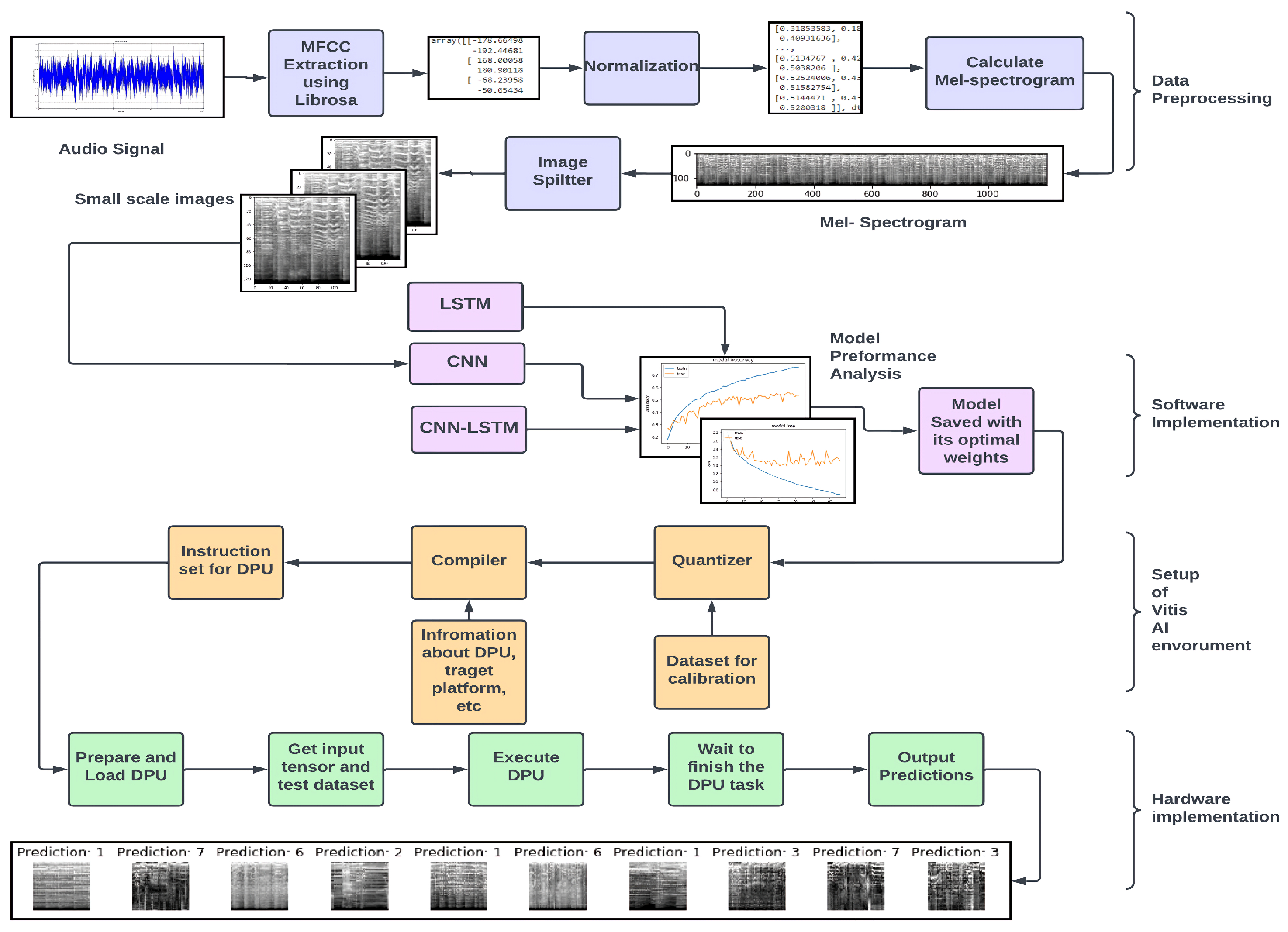
In this section, we describe our proposed deep-learning-based music genre classification system using the ZCU104 Evaluation Kit. The overall process can be divided into four major parts: data preprocessing, software implementation of deep learning models, setup of the Vitis AI environment, and hardware implementation of the models on the ZCU104 Evaluation Kit.
Data preprocessing included the extraction of audio features and normalization of signals. The extracted features were then used to train and test three different deep learning models, namely convolutional neural network (CNN), long short-term memory (LSTM), and CNN-LSTM. These models were compared in the software implementation. Then, the Vitis AI environment was set up to enable the implementation of the trained models on the FPGA board. Finally, the hardware implementation of the deep learning models was carried out on the ZCU104 Evaluation Kit.
Overall, we provide a comprehensive approach for implementing deep-learning-based music genre classification on the ZCU104 Evaluation Kit as shown in
Figure 1. A detailed explanation of each part of our proposed method is provided in the following sections.
3.1. Dataset
The GTZAN dataset [
9] created by George Tzanetakis is widely employed in the development of machine learning and deep learning models for music classification. The dataset consists of 1000 audio clips, each with a duration of 30 s, spanning ten different genres of music, including blues, classical, country, disco, hip-hop, jazz, metal, pop, reggae, and rock. Each genre is represented by 100 audio clips in “.wav” format, and the dataset is publicly available for researchers to use [
9]. The dataset serves as a benchmark to evaluate the performance of various music classification models and has been utilized by many researchers, making it a well-established resource in music classification research. The GTZAN dataset can be conveniently downloaded from Kaggle [
10].
3.2. Mel-Frequency Cepstral Coefficient
We evaluated different feature representations for music genre classification and conclude that Mel-frequency cepstral coefficients (MFCCs) are the most suitable feature for this task. Our decision to use MFCCs was based on the work presented in the literature review section, where it was shown that MFCCs have been commonly used in music classification tasks and are robust to variations in the signal’s overall level and spectral content.
MFCCs are derived from the short-time Fourier transform (STFT) of an audio signal and capture the spectral (frequency) characteristics of the signal that are important for human hearing. They are calculated by taking the log magnitude of the STFT, performing a discrete cosine transform (DCT) on the resulting coefficients, and taking the first few coefficients of the DCT.
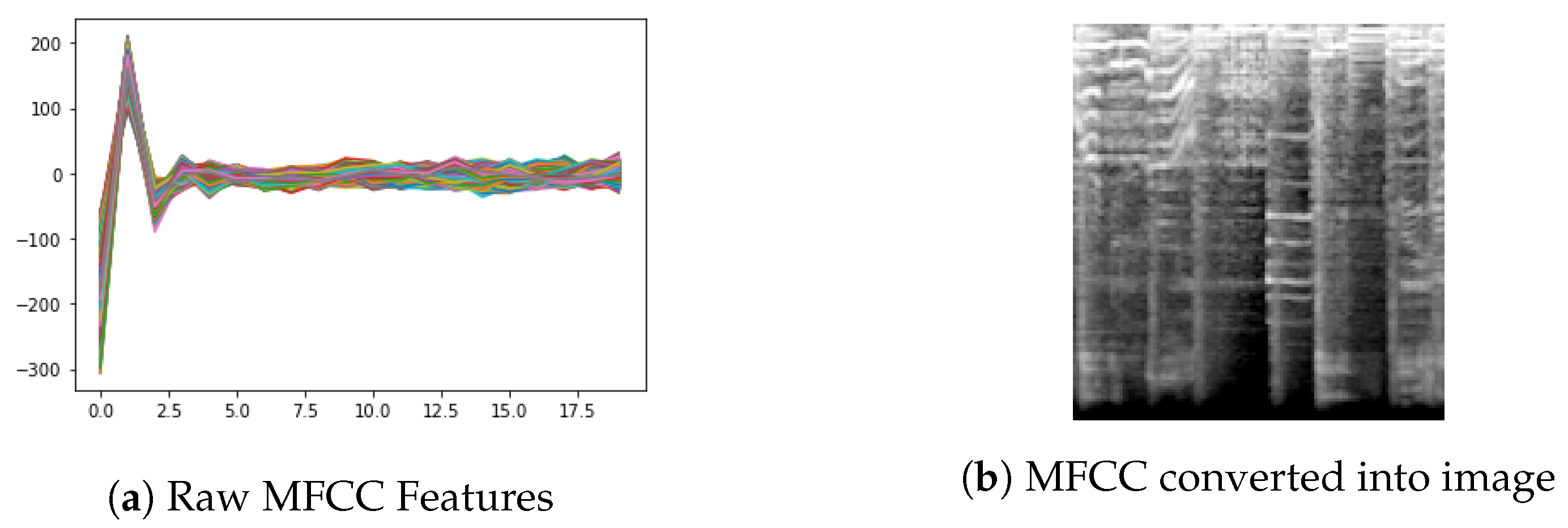
In this study, we utilized MFCCs to train and evaluate deep learning models for music genre classification. We used raw coefficients (as shown in
Figure 2a) to train the LSTM model and image representations (as shown in
Figure 2b) of MFCCs to train the CNN and hybrid (CNN-LSTM) models as shown in
Figure 3. This approach allowed us to leverage the strengths of different deep learning models to achieve better results in music classification and provide a comparative analysis.
3.3. Our Proposed Architectures
Our proposed architectures for music genre classification include three distinct deep learning models: long short-term memory (LSTM), convolutional neural network (CNN), and a hybrid model that combines both CNN and LSTM architectures. Each of these models was thoroughly evaluated to determine their effectiveness in performing music classification tasks. Ultimately, the CNN model was chosen for deployment on the SoC-FPGA due to its superior performance and manageable number of trainable parameters. The choice was also limited by hardware restrictions, as only the CNN model could be executed on SoC-FPGA using the deep learning processing unit (DPU).
3.3.1. LSTM Architecture
In our LSTM architecture as shown in
Figure 4, two LSTM layers are used to capture the sequential dependencies between the MFCC features and the music genre labels. Each LSTM layer consists of 100 LSTM cells. These layers process the input MFCC data and learn the complex relationships between the features and the target labels. The output of the LSTM layers is then fed into two fully connected layers, which make the final prediction about the genre of the input music.
3.3.2. CNN Architecture
The CNN model used here is structured with multiple CNN layers followed by pooling layers specifically designed for image classification tasks as shown in
Figure 5. This model was adapted for the music classification task by feeding MFCC arrays, represented as images, into the model, allowing the CNN to extract features and make predictions with respect to the genre of a musical piece.
3.3.3. CNN-LSTM Architecture
The hybrid model shown in
Figure 6 combines CNN and LSTM algorithms to improve the results for complex tasks in deep learning. The CNN extracts relevant features from the audio stream, while the LSTM models the temporal dependencies between these features. The combination of the two models allows for proper management of both spatial and temporal information in the audio source. The CNN reduces complexity by extracting the most relevant features, and the LSTM preserves the temporal correlations between these elements.
The chosen model for hardware implementation is the CNN model due to its superior performance and computational efficiency compared to the LSTM and CNN-LSTM models. The CNN model is also less complex than the other models, making it easier to interpret and implement on FPGA. However, it is important to note that this choice was also made due to hardware limitations, as only the CNN model could be executed on the FPGA.
In summary, we have proposed three distinct deep learning models for music classification: LSTM, CNN, and a hybrid model combining both CNN and LSTM architectures. After thorough evaluation, the CNN model was chosen for deployment on the SoC-FPGA due to its superior performance and computational efficiency. The LSTM and CNN-LSTM models have the potential to capture the temporal features of data, but the CNN model outperforms the other models in terms of accuracy and computational efficiency.
3.4. Vitis AI
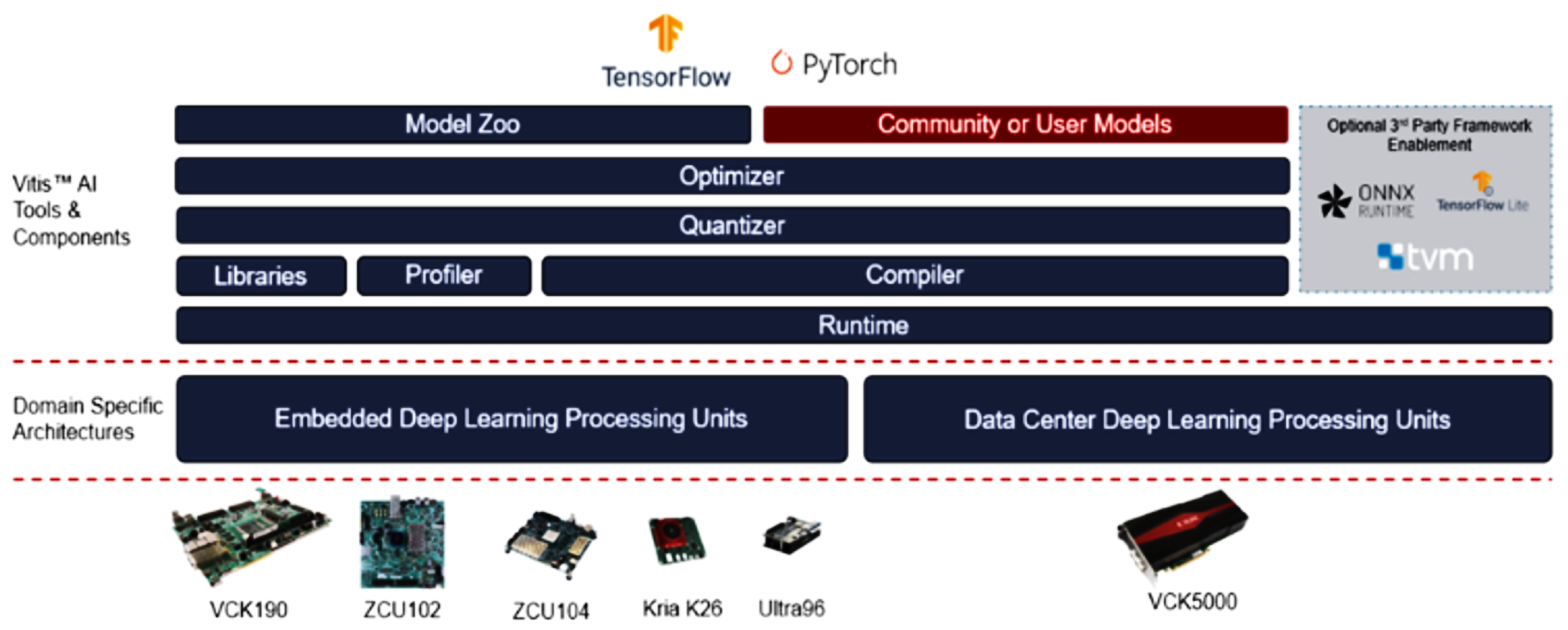
The Vitis AI development environment is an integrated toolkit aimed at boosting the performance of AI inference on Xilinx hardware platforms as shown in
Figure 7. It is an all-in-one solution that provides everything needed to develop AI applications on Xilinx systems-on-chips (SoCs) and adaptive compute acceleration platforms (ACAPs). The environment comprises a suite of optimized IP cores, tools, libraries, models, and example designs. These resources are designed with the goal of maximizing efficiency and simplifying the development process for users—even those without a background in FPGA technology. The Vitis AI development environment is engineered to hide the complex programming details of FPGA technology, allowing developers to focus on creating deep learning inference applications with ease [
11].
The proposed system is executed using two advanced tools: the Vitis AI quantizer and compiler. In addition, Vitis AI’s preimplemented IP core, the deep learning processing unit (DPU), speeds up the system’s development time. The Vitis AI quantizer and compiler help to optimize the deep learning algorithms, while the DPU is a specialized IP core optimized to execute these algorithms. These tools and the DPU were used in this work with the aim of unleashing the full potential of AI acceleration on Xilinx SoC FPGA as shown in
Table 3.
4. Implementation
This section discusses the software implementation of three deep learning models for music classification (LSTM, CNN, and CNN-LSTM), including data preprocessing and model architecture implementation. It also describes the Vitis AI work flow for quantization and compilation of models for deployment on Xilinx hardware. The entire system is implemented using Python and its available libraries. The second part of this section focuses on the hardware system’s design and implementation, including selection of the appropriate DPU, design of the system architecture, and system implementation for the deployment of the CNN model. This section culminates with a whole hardware system design from beginning to end.
4.1. Software Implementation
In this section, we start by providing the details of data preparation for the proposed models, followed by a description of the development of the CNN, LSTM, and CNN-LSTM models. Then, the design flow of each model is provided, followed by the work flow of Vitis AI.
4.1.1. Data Preprocessing
In this study, MFCCs are used for music classification. MFCC features are extracted using a Python library called Librosa as shown in
Figure 8. The library provides a comprehensive set of audio processing functions, including audio visualization, time-frequency analysis, and audio extraction features. To extract MFCC features, the audio file is loaded into the program, and librosa.feature.mfcc() generates a multidimensional MFCC array. This array contains raw MFCC features that are not normalized. Data normalization plays a crucial role in deep learning, as it alters the range of data points, helping the model to find its global minimum. To implement normalization, the preprocessing package provided by sklearn is used. The data are normalized using sklearn.preprocessing.MinMaxScaler(), which scales the range of MFCC features from 0 to 1. These calculated MFCC features are then passed to librosa.feature.melspectrogram() to compute a Mel-scaled spectrogram.
Data augmentation is used to expand the dataset by creating new data points from existing data. In this work, the technique of image splitting is used, which involves dividing an image of the Mel-Spectrogram (with the shape of (128, 1200)) into equally spaced small images of shape (128, 120) as shown in
Figure 9. This technique helps to increase the amount of available data, which can improve the accuracy and generalization capability of machine learning models. With this method, the number of images is increased by 1000 per class, corresponding to 10,000 images of the Mel-spectrogram for 10 classes.
4.1.2. Model Implementation
This work presents the development of three models for comparative analysis: LSTM, CNN, and a hybrid model (CNN-LSTM).
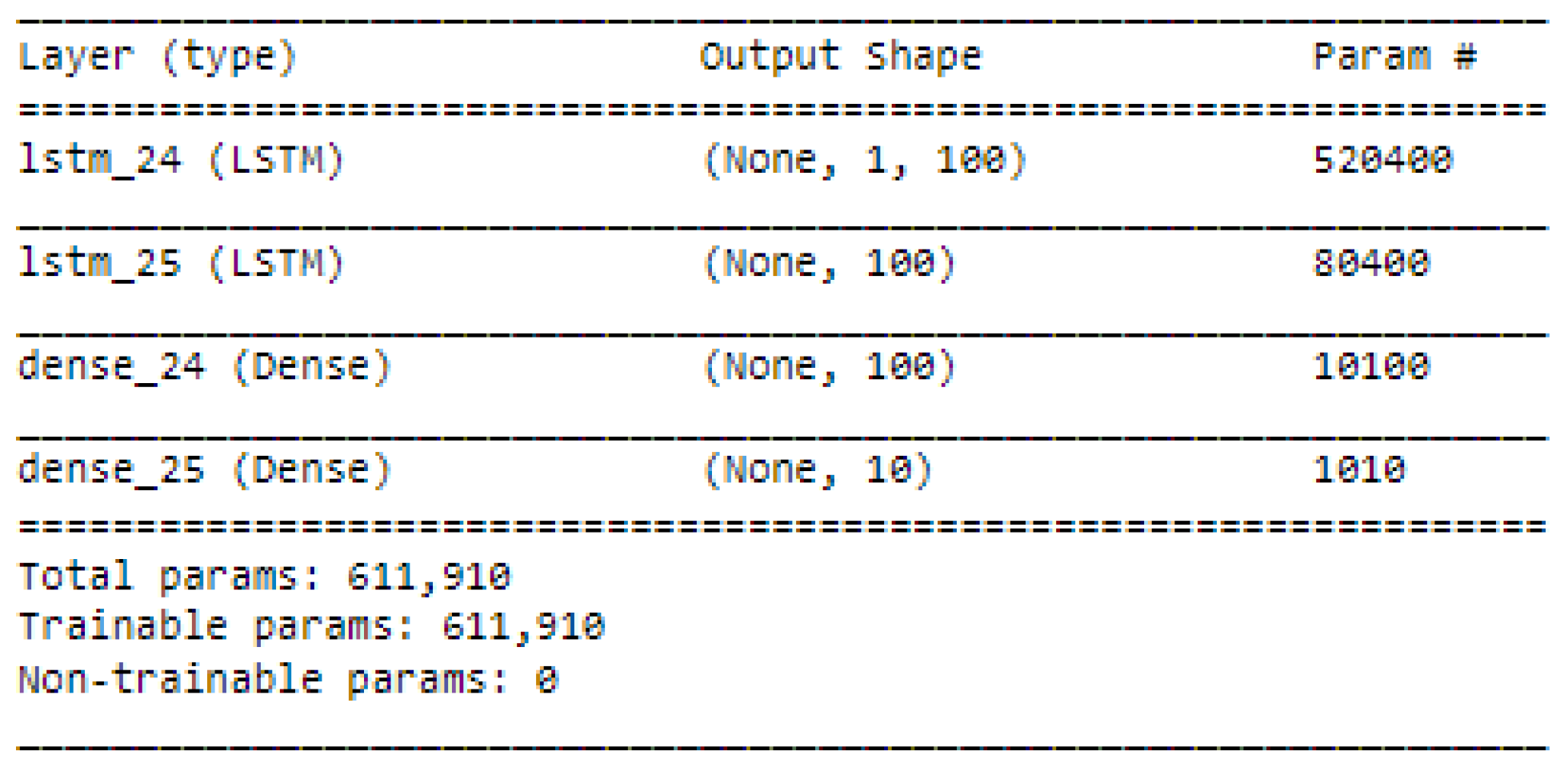
The LSTM model consists of an input layer that takes 1200 features one by one followed by two LSTM layers, each with 100 units as shown in
Figure 10. The first LSTM layer receives an input with a shape of (1, 1200) and outputs data with a shape of (1, 100) through its 100 units, passing the data to the next LSTM layer. After learning the relationship between the features and labels, the data pass through a block of fully connected layers to output the probability distribution of each class.
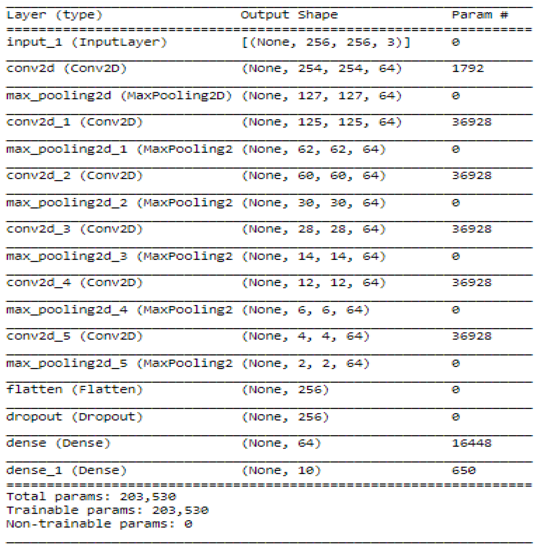
The proposed CNN architecture consists of six CNN blocks, each with a CNN layer followed by a max pooling layer as shown in
Figure 11. After CNN blocks, the captured features pass through a flatten layer, which transforms the features into a single dimension. A dropout layer with a 50% dropout rate is used between the flatten layer and the fully connected block to introduce regularization, which reduces overfitting of the model. The dropout layer randomly drops out a certain percentage of neurons during training, helping to prevent the model from memorizing the training data.
The hybrid model (CNN-LSTM) combines both the CNN and LSTM models as shwon in
Figure 12. The output of the CNN layer is passed to the LSTM layer, which then passes the output to the fully connected layers to output the probability distribution of each class.
Four CNN computational blocks. In each block, a CNN layer is used for feature extraction, followed by a max pooling layer to capture the most prominent feature set.
The output of the CNN block is then reshaped using a reshape layer. This changes a 3D CNN output to a 2D LSTM input.
An LSTM layer is introduced to learn time-dependent features from the data provided by the CNN block.
Finally, a flatten layer followed by two fully connected layers is utilized to output the probability distribution of the classes.
4.1.3. Design Flow for Proposed Models
The proposed models are implemented by one of the leading deep learning frameworks, TensorFlow. Here, we present the implementation and work flow for the proposed LSTM, CNN, and hybrid (CNN-LSTM) models. Further, the combined implementation of CNN and the hybrid model (CNN-LSTM) is discussed, as both models them utilize CNN layers at the beginning of the model.
LSTM Design Flow
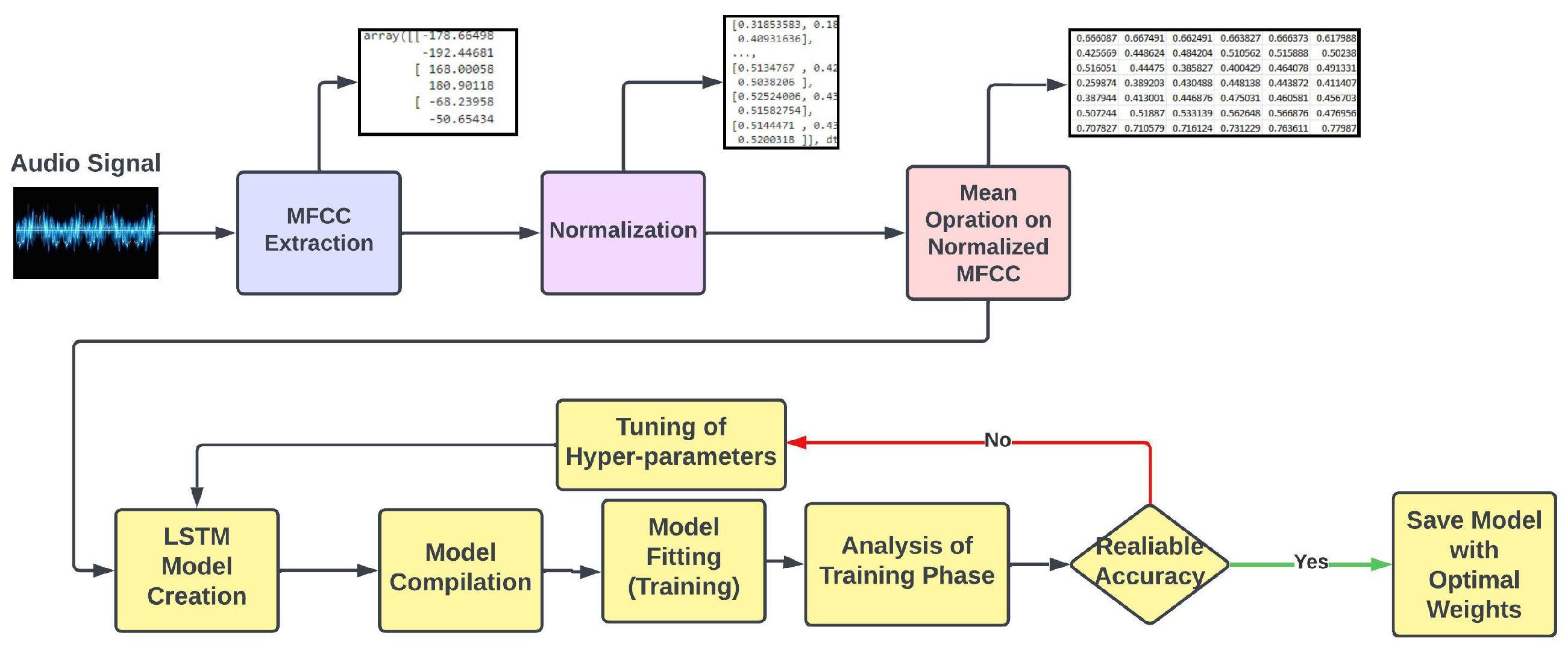
The work flow for the implementation of the LSTM model is illustrated in the
Figure 13. It starts by loading the audio files, followed by data preprocessing. First, the extraction of MFCC features takes place, followed by data normalization. As we discussed earlier, MFCCs are high-dimensional features. In order to make these features compatible with the LSTM model, we take the mean (average) value of each MFCC feature to train the model in a reasonable time. The extracted raw MFCCs have the shape of (128, 1200) for each audio file, resulting in an enormous amount of time for training. By taking the mean of MFCCs, the new shape for each audio file is (1, 1200), where the first dimension (1) represents the average value of 128 MFCCs over 1200 data points (time stamps). Utilizing this method addresses the high-dimensionality problem. The final reduced dataset has the shape of (1000, 1200), where 1000 represents the average-valued MFCC of 1000 audio files with time stamps of 1200.
The proposed LSTM model is implemented using TensorFlow.
Figure 13 shows the steps taken in developing the model. It starts by defining the model architecture. Once a baseline architecture is created, we compile the model. When compiling the model, we specify the loss function, optimizer, and matrix that we want to monitor during the training phase. Here, we use Adam as an optimizer with a learning rate of 0.001. The loss function is
sparse_categorical_crossentropy, and we monitor the matrix of accuracy while training.
The Adam optimizer is commonly used in training LSTM models [
12]. Adam optimization is a type of stochastic gradient descent method that utilizes the estimation of first-order and second-order moments in an adaptive manner [
13]. Sparse categorical cross entropy calculates the cross-entropy loss between labels and predictions. This loss function is utilized in response to the multiclass classification problem [
14].
The development of deep learning models requires a trial-and-error method. After analyzing the model performance, it needs to update. This process is also called hyperparameter tuning. This tuning helps the developers to achieve a balance between underfitting and overfitting [
15]. Once the model achieves a reliable accuracy or starts overfitting, it is saved with its optimal weights.
CNN and Hybrid Model Work Flow
The design flows of the CNN and hybrid (CNN-LSTM) models start with the same preprocessing technique as shown in
Figure 14. Initially, the audio file is loaded into the program, and the MFCC features are extracted utilizing the built-in functions provided by Librosa. To alter the range of the raw MFCCs, the system normalizes the data, followed by the generation of the Mel-spectrogram. After producing the Mel-spectrogram, it passes over an image splitter, which splits the large images into smaller images of the spectrogram, resulting in an increased number of images.
The model fed with these images along with their labels. Both the CNN and hybrid (CNN-LSTM) models are implemented using TensorFlow. After defining the models, they are compiled. To compile the models, root mean square propagation (RMSProp) and categorical cross entropy are used as an optimizer and loss function, respectively.
RMSProp is an optimizer that is effective for deep neural networks and improves the ability to handle extremely small learning rates as the training progresses. This optimizer is often used to train CNNs and performs better as compared to other optimizers for image recognition [
16]. Categorical cross entropy calculates the cross-entropy loss between true labels and predicted labels. This function is best-suited for multiclass classification [
17].
4.1.4. Vitis AI Work Flow
Vitis AI smooths down the process of deployment. This framework is specifically designed for deep learning developers to run and test their models without going into the intricacies of FPGA programming and development. In this project, we used Vitis AI version 1.4, which can be downloaded from DockerHub [
18].
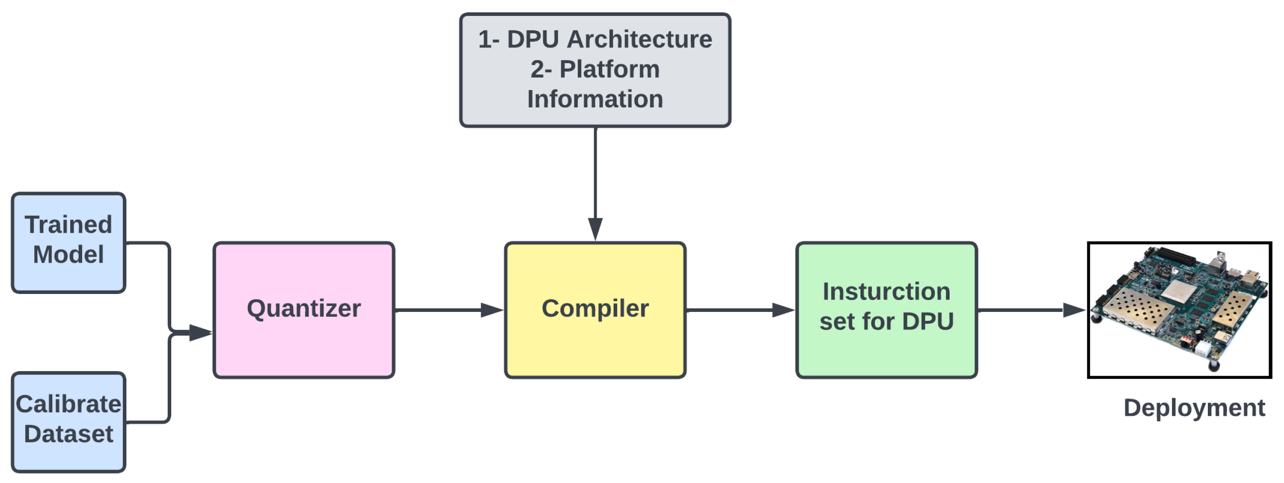
The design flow shown in
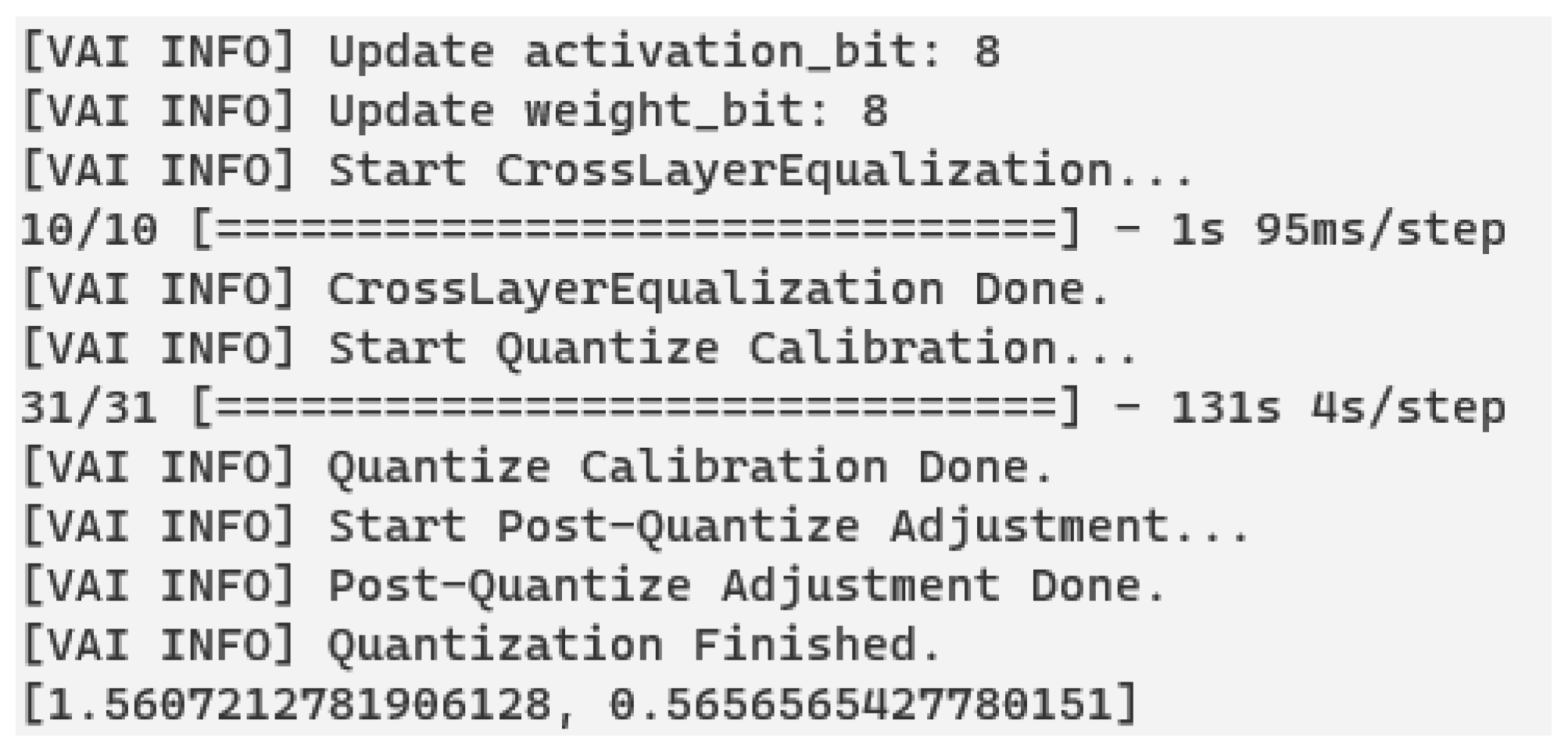
Figure 15 starts by providing the trained model and a calibration dataset to the Vitis AI quantizer. The quantizer receives a trained model with weights and floating-point 32-bit data and converts the model weights into integer 8 bits. During this process, the quantizer shown in
Figure 16 uses a small part of the dataset to calibrate the weight to achieve the maximum model performance. The process of quantization always eliminates some information from the model; however, by utilizing a calibration dataset, the quantizer can reduce the model size by half without compromising much on the accuracy.
The quantized model is then forwarded to the Vitis AI compiler. The compiler computes a highly efficient instruction set that the DPU can execute based on the provided model. It also takes some other input, such the DPU architecture, platform information, and output directory. Here, we use DPUCZDX8G and ZUC104 as the DPU architecture and target platform, respectively. Following compilation shown in
Figure 17, the model is ready for deployment on the FPGA.
4.2. Hardware Implementation
Now, we describe the implementation of the CNN-based music classifier on SoC-FPGA.
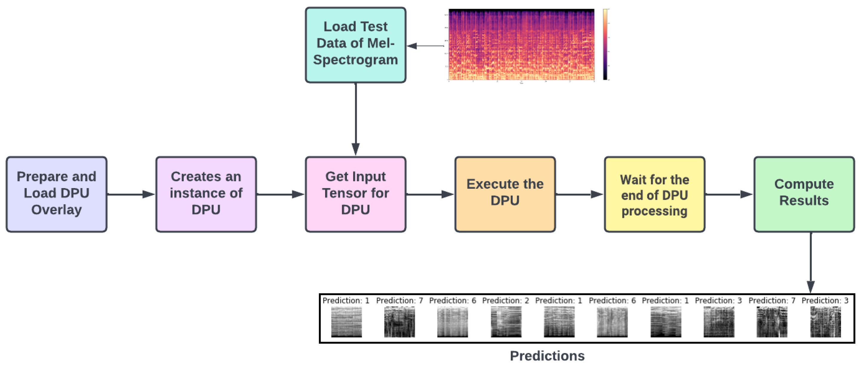
Several steps are involved in the FPGA work flow for to implement deep learning models as shown in
Figure 18. These steps are as follows:
Prepare and load the DPU overlay: The DPU overlay must be prepared and loaded onto the FPGA before it can be used. The DPU IP and its associated configuration parameters are stored in the overlay;
Create a DPU instance: Once the overlay has been loaded, a DPU instance must be created. The deep learning model is run on this instance;
Obtain the DPU’s input tensor: The DPU’s input tensor must be provided. The testing dataset is fed into the DPU in this step. The input data are then preprocessed and sent to the DPU in the appropriate format;
Execute the DPU: The deep learning model is then run using the DPU. The deep learning model is applied to the input tensor by the DPU, and the output tensor is produced;
Wait for the DPU to finish its job: The FPGA waits for the DPU to finish its job. The DPU’s execution time is determined by the model’s complexity and the size of the input data.
Compute results: After the DPU has finished its work, the results are computed. Based on the deep learning model, the output tensor is analysed to make predictions or classify the data.
The work flow to implement deep learning models on FPGA includes loading the DPU overlay, creating an instance of the DPU, providing input data, executing the DPU, waiting for the DPU to finish its job, and computing the results. These steps are required for efficient deep learning model execution on FPGAs.
5. Results and Analysis
The results and analysis of experiments conducted to evaluate the performance of the LSTM, CNN, and CNN-LSTM models in music classification are presented in this section. A detailed comparison of the model complexities and the number of trainable parameters of the three models, followed by an analysis of their accuracy on the testing dataset in the software results section, are presented below. Additionally, the hardware results section presents a performance evaluation of the FPGA-based CNN model implementation, focusing on its execution time and resource utilization.
5.1. Model Complexity
Analysis of the number of learnable parameters in deep learning models is essential to comprehend the model’s operations and its ability to process input data. This metric is pivotal in determining the complexity and capacity of deep learning models. To avoid underfitting or overfitting, it is crucial to monitor the number of parameters in each layer. Thus, keeping track of the number of parameters is a crucial step to ensure the effectiveness and efficiency of deep learning models. Several studies have shown that the number of parameters in a model influences its performance, and optimizing this number is crucial to obtain accurate results [
19].
Comparison and Analysis of Model Complexity
The size of a deep learning model is directly proportional to its number of trainable parameters. The inference time of a model, which is the time it takes to make a prediction, is also influenced by the number of parameters in the model. Generally, models with more parameters take longer to make predictions. Additionally, the computational cost of running a larger model is higher than that of running a smaller model with fewer parameters. This results in a greater demand for energy and storage space when using models with more trainable parameters. To put it simply, the larger the model, the more energy, time, and memory space it requires [
20].
Table 4 depicts a comparative analysis between the three proposed models. The figures show that CNN has the fewest trainable parameters as compared to the LSTM and CNN-LSTM models. In the context of testing accuracy, our results show that CNN has the best testing accuracy among the presented models. This makes the CNN model our choice to implement on the FPGA. However, because the CNN model is the least complex, it provides the best testing accuracy.
5.2. Software Results
The performance of a deep learning model is affected by various factors, such as the model type, the quality and quantity of data used for training, and the hardware platform utilized for testing and training. In this section, we present an analysis and comparison of the performance of three music classification models: the LSTM, CNN, and hybrid (CNN-LSTM) models. The evaluation is based on accuracy of the models in training and testing and their execution time on an Intel Core i7-8550U. The platform used to train the models is also considered, as it can impact their performance. By analyzing these metrics, we can gain insights into the strengths and weaknesses of each model and determine which one is best-suited for hardware implementation.
The models (LSTM, CNN, and hybrid) are compared based on their training and testing accuracy and execution time.
Table 5 provides a detailed analysis. The following points summarize the key insights of the information provided in the table.
Platform for Training: This row shows the platform used to train the models. The CNN and hybrid models were trained on Google Cloud Engine (GCE), while the LSTM model was trained on an Intel Core i7-8550U;
Training Accuracy: This row displays the percentage of correct predictions made by the models during training. The CNN and hybrid models outperform the LSTM model in terms of training accuracy (99%). This suggests that the CNN and hybrid models capture more information from the training data;
Testing Accuracy: This row shows the percentage of correct predictions generated by the models on unseen data. The LSTM model has a significantly lower testing accuracy (22%) than the CNN and hybrid models (57% and 56%, respectively). This indicates that the LSTM model may not generalize well to new data;
Execution Time: This row displays how long each model takes to make predictions on the Intel Core i7-8550U. The LSTM model takes the least time to execute (1.48 s), while the CNN model takes the longest time (25.96 s). The execution time of the hybrid model is intermediate (18.99 s).
5.3. FPGA Results
In this work, the performance of a CNN model is compared on two different platforms (a Zynq UltraScale+ MPSoC ZCU104 Evaluation Kit and an Intel Core i7-8550U) in terms of testing accuracy, execution time, and throughput. The results show that SoC-FPGA outperforms Intel Core i7-8550U, making FPGA an excellent choice for deep learning model implementation.
A CNN model was tested on two separate systems (a Zynq UltraScale+ MPSoC ZCU104 Evaluation Kit and an Intel Core i7-8550U), as shown in
Table 6.
In terms of testing accuracy, the CNN model only lost less than 1% of test accuracy on the Zynq UltraScale+ MPSoC ZCU104 Evaluation Kit as compared to the Intel Core i7-8550U (57% and 56.56% on the Intel Core i7-8550U and Zynq UltraScale+ MPSoC ZCU104 Evaluation Kit, respectively).
However, in terms of execution time, the Zynq UltraScale+ MPSoC ZCU104 Evaluation Kit surpassed the Intel Core i7-8550U, with a time of 5.13 s versus 25.96 s for the Intel Core i7-8550U. This shows that where low latency is required, the CNN model is better-suited for implementation on the Zynq UltraScale+ MPSoC ZCU104 Evaluation Kit.
The CNN model’s throughput was also greater on the Zynq UltraScale+ MPSoC ZCU104 Evaluation Kit, with 192 images per second compared to 38 on the Intel Core i7-8550U. This means that the Zynq UltraScale+ MPSoC ZCU104 Evaluation Kit can process more frames per second, making it better-suited for real-time video processing applications.
6. Conclusions
In this paper, we designed and implemented a real-time system for music genre classification using deep learning on a SoC-FPGA device. The system includes a data preprocessing stage; MFCC audio feature extraction; and neural network classification using LSTM, CNN, and CNN-LSTM models.
A comparison of the three models shows that the CNN and hybrid models outperform the LSTM model in terms of training and testing accuracy. Although LSTM has the shortest execution time, CNN is chosen for hardware implementation due to its less complex architecture and high test accuracy, making it suitable for SoC-FPGA. However, the implementation of the LSTM and hybrid (CNN-LSTM) models is not supported by the DPU running on the SoC-FPGA, limiting their evaluation on the FPGA board.
Overall, this work shows that SoC-FPGA devices can be used for classification tasks using deep learning models. On the GTZAN dataset, the CNN models can achieve a classification accuracy of up to 56% in 5.13 s, demonstrating the feasibility of this approach. The hardware platform of choice is determined by the specific application requirements, with the Zynq UltraScale+ MPSoC ZCU104 Evaluation Kit offering lower latency and higher throughput than the Intel Core i7-8550U, which only slightly outperforms the former in terms of testing accuracy.
Certain constraints exist in the proposed system, which should be addressed in future work. For example, the proposed system is based on a low-cost and low-power SoC-FPGA device, which may limit the scalability and computational capabilities of the developed models. The performance can be improved further if a more advanced platform or design tool is available.
In summary, this research lays the foundation for the utilization deep learning on SoC-FPGA devices for real-time classification tasks. This approach can be used for other similar classification tasks in broader applications.
Author Contributions
Conceptualization, H.M.; methodology, M.F., I.C. and H.M.; software, M.F.; validation, M.F., I.C., H.M. and I.I.; formal analysis, M.F.; investigation, M.F.; resources, M.F.; data curation, M.F.; writing—original draft preparation, M.F. and I.I.; writing—review and editing, M.F., I.I. and H.M.; visualization, M.F.; supervision, H.M.; project administration, H.M.; funding acquisition, H.M. All authors have read and agreed to the published version of the manuscript.
Funding
This Research was funded by British Heart Foundation under number of FS/19/73/34690.
Institutional Review Board Statement
Not applicable.
Informed Consent Statement
Not applicable.
Data Availability Statement
Conflicts of Interest
The authors declare no conflict of interest.
References
- Chen, R.; Wu, T.; Zheng, Y.; Ling, M. MLoF: Machine Learning Accelerators for the Low-Cost FPGA Platforms. Appl. Sci. 2022, 12, 89. [Google Scholar] [CrossRef]
- Ashraf, M.; Geng, G.; Wang, X.; Ahmad, F.; Abid, F. A Globally Regularized Joint Neural Architecture for Music Classification. IEEE Access 2020, 8, 220980–220989. [Google Scholar] [CrossRef]
- Fulzele, P.; Singh, R.; Kaushik, N.; Pandey, K. A Hybrid Model for Music Genre Classification Using LSTM and SVM. In Proceedings of the 2018 Eleventh International Conference on Contemporary Computing (IC3), Noida, India, 2–4 August 2018; pp. 1–3. [Google Scholar] [CrossRef]
- Yi, Y.; Zhu, X.; Yue, Y.; Wang, W. Music Genre Classification with LSTM based on Time and Frequency Domain Features. In Proceedings of the 2021 IEEE 6th International Conference on Computer and Communication Systems (ICCCS), Chengdu, China, 23–26 April 2021; pp. 678–682. [Google Scholar] [CrossRef]
- Khasgiwala, Y.; Tailor, J. Vision Transformer for Music Genre Classification using Mel-frequency Cepstrum Coefficient. In Proceedings of the 2021 IEEE 4th International Conference on Computing, Power and Communication Technologies (GUCON), Kuala Lumpur, Malaysia, 24–26 September 2021; pp. 1–5. [Google Scholar] [CrossRef]
- Hassan, R.O.; Mostafa, H. Implementation of deep neural networks on FPGA-CPU platform using Xilinx SDSOC. Analog Integr. Circuits Signal Process. 2021, 106, 399–408. [Google Scholar] [CrossRef]
- Yoshimura, U.; Inoue, T.; Tsuchiya, A.; Kishine, K. Implementation of Low-Energy LSTM with Parallel and Pipelined Algorithm in Small-Scale FPGA. In Proceedings of the 2021 International Conference on Electronics, Information, and Communication (ICEIC), Jeju, Republic of Korea, 31 January–3 February 2021; pp. 1–4. [Google Scholar] [CrossRef]
- Ushiroyama, A.; Watanabe, M.; Watanabe, N.; Nagoya, A. Convolutional neural network implementations using Vitis AI. In Proceedings of the 2022 IEEE 12th Annual Computing and Communication Workshop and Conference (CCWC), Las Vegas, NV, USA, 26–29 January 2022; pp. 0365–0371. [Google Scholar] [CrossRef]
- Tzanetakis, G.; Essl, G.; Cook, P. Automatic Musical Genre Classification of Audio Signals. In Proceedings of the 2nd International Symposium on Music Information Retrieval, Bloomington, IN, USA, 15–17 October 2001. [Google Scholar]
- Olteanu, A. GTZAN Dataset: Music Genre Classification. 2020. Available online: https://www.kaggle.com/andradaolteanu/gtzan-dataset-music-genre-classification (accessed on 30 April 2023).
- Vitis AI Overview. Vitis AI User Guide (UG1414). Reader. Documentation Portal. Available online: https://docs.xilinx.com/r/en-US/ug1414-vitis-ai/Vitis-AI-Overview (accessed on 30 April 2023).
- Chang, Z.; Zhang, Y.; Chen, W. Effective Adam-Optimized LSTM Neural Network for Electricity Price Forecasting. In Proceedings of the 2018 IEEE 9th International Conference on Software Engineering and Service Science (ICSESS), Beijing, China, 23–25 November 2018; pp. 245–248. [Google Scholar] [CrossRef]
- Keras-Adam. Available online: https://keras.io/api/optimizers/adam/ (accessed on 30 April 2023).
- Keras-Sparsecategoricalcrossentropy-Class. Available online: https://keras.io/api/losses/probabilistic_losses/#sparsecategoricalcrossentropy-class (accessed on 30 April 2023).
- Hyper-Parameter Tuning Techniques in Deep Learning | by Javaid Nabi | Towards Data Science. Available online: https://towardsdatascience.com/hyper-parameter-tuning-techniques-in-deep-learning-4dad592c63c8 (accessed on 30 April 2023).
- Bae, S.H.; Kwon, C.K. Comparison Study of Optimizer on CNN based Finger Number Recognition using sEMG Signals. In Proceedings of the 2021 International Conference on Computational Science and Computational Intelligence (CSCI), Las Vegas, NV, USA, 15–17 December 2021; pp. 1750–1751. [Google Scholar] [CrossRef]
- Keras-Categorical Crossentropy. Available online: https://keras.io/api/losses/probabilistic_losses/#categoricalcrossentropy-class (accessed on 30 April 2023).
- VitisAI-Docker. Available online: https://hub.docker.com/r/xilinx/vitis-ai (accessed on 30 April 2023).
- LSTM: Understanding the Number of Parameters | Kaggle. Available online: https://www.kaggle.com/code/kmkarakaya/lstm-understanding-the-number-of-parameters (accessed on 30 April 2023).
- Pokhrel, S. Model Compression: Needs and Importance | by Sabina Pokhrel | Towards Data Science. Available online: https://towardsdatascience.com/model-compression-needs-and-importance-6e5913996e1 (accessed on 30 April 2023).
Figure 1.
Overview of the proposed methodology with four stages: Data preprocessing; software implementation; setup of the Vitis AI environment; and hardware implementation.
Figure 1.
Overview of the proposed methodology with four stages: Data preprocessing; software implementation; setup of the Vitis AI environment; and hardware implementation.
Figure 2.
Difference between raw and image-based MFCCs. The raw MFCC features are used as time steps in the LSTM model, whereas the CNN model uses the converted version of the MFCC.
Figure 2.
Difference between raw and image-based MFCCs. The raw MFCC features are used as time steps in the LSTM model, whereas the CNN model uses the converted version of the MFCC.
Figure 3.
Extraction and conversation of MFCC features and their utilization in LSTM, CNN and hybrid (CNN-LSTM) models.
Figure 3.
Extraction and conversation of MFCC features and their utilization in LSTM, CNN and hybrid (CNN-LSTM) models.
Figure 4.
Proposed LSTM architecture. We used the extracted MFCC features and fed them into two consecutive LSTM layers, each consisting of 100 LSTM cells. In the end, we took the result from the last LSTM layer and fed it into a fully connected layer of 10 neurons, which provides the classification label.
Figure 5.
Proposed CNN architecture with six CNN blocks followed by a flatten and dropout layer. Each CNN block consists of a CNN layer and a max pooling layer. Fully connected layers are used to predict the music genre. The model uses MFCCs as input features.
Figure 5.
Proposed CNN architecture with six CNN blocks followed by a flatten and dropout layer. Each CNN block consists of a CNN layer and a max pooling layer. Fully connected layers are used to predict the music genre. The model uses MFCCs as input features.
Figure 6.
The proposed CNN-LSTM architecture takes MFCC features as input and consists of a CNN block that captures the spatial Mel-spectrogram features and an LSTM block that captures the temporal Mel-spectrogram features. The probability distribution of each genre class is then defined using fully connected layers.
Figure 7.
Vitis AI integrated development environment [
11].
Figure 7.
Vitis AI integrated development environment [
11].
Figure 8.
Extraction of MFCCs. The process starts by loading and calculating MFCCs, followed by normalization of the raw features. Finally, a Mel-spectrogram is generated based on the MFCC features.
Figure 8.
Extraction of MFCCs. The process starts by loading and calculating MFCCs, followed by normalization of the raw features. Finally, a Mel-spectrogram is generated based on the MFCC features.
Figure 9.
Image splitter used to deal with the limited dataset. It takes a large image of the Mel-spectrogram of shape (128, 1200) and divides each image into 10 small images of shape (128, 120).
Figure 9.
Image splitter used to deal with the limited dataset. It takes a large image of the Mel-spectrogram of shape (128, 1200) and divides each image into 10 small images of shape (128, 120).
Figure 10.
LSTM model summary.
Figure 10.
LSTM model summary.
Figure 11.
CNN model summary.
Figure 11.
CNN model summary.
Figure 12.
CNN-LSTM model summary.
Figure 12.
CNN-LSTM model summary.
Figure 13.
The LSTM model for music classification begins with data preprocessing, which includes MFCC feature extraction and data normalization. The high-dimensionality problem is solved by taking the average value of each MFCC feature, and the reduced dataset is used to train the LSTM model, which uses the Adam optimizer and the sparse categorical cross-entropy loss function to achieve multiclass classification.
Figure 14.
The same preprocessing technique is used by both CNN and hybrid (CNN-LSTM) models, beginning with loading and extraction of MFCC features from audio files. The number of images is increased using image splitters, and images are compiled using root mean square propagation (RMSProp) as an optimizer and categorical cross entropy as the loss function.
Figure 15.
Vitis AI makes deep learning model deployment on FPGA easier by providing a framework that eliminates the need for FPGA programming and development. The deployment process begins with the Vitis AI quantizer, which converts the trained model weights into integer 8 bits, followed by the Vitis AI compiler, which generates an efficient instruction set for the DPU to execute. Finally, the model is deployed on the FPGA.
Figure 16.
Output of the Vitis AI quantizer.
Figure 16.
Output of the Vitis AI quantizer.
Figure 17.
Output of the Vitis AI compiler.
Figure 17.
Output of the Vitis AI compiler.
Figure 18.
Preparing and loading the DPU overlay, creating a DPU instance, providing input data to the DPU, executing the DPU, waiting for the DPU to finish its job, and computing the results based on the DPU’s output tensor are all steps in running a deep learning model on an FPGA with a DPU.
Figure 18.
Preparing and loading the DPU overlay, creating a DPU instance, providing input data to the DPU, executing the DPU, waiting for the DPU to finish its job, and computing the results based on the DPU’s output tensor are all steps in running a deep learning model on an FPGA with a DPU.
Table 1.
Comparison between different models applied on two datasets (GTZAN and FMA) extracted from the literature.
Table 1.
Comparison between different models applied on two datasets (GTZAN and FMA) extracted from the literature.
| Research | Model Architecture | Dataset | Features | Test Accuracy |
|---|
| [2] | CNN-RNN combined with global layer regulation | GTZAN | MFCC | 87.79 |
| [2] | CNN-RNN combined with global layer regulation | FMA | MFCC | 68.87 |
| [3] | LSTM + SVM | GTZAN | SSD, MFCC, Spectral Roll Off, ZCR, Chroma Frequency, Rhythm Histogram, and Spectral Centroid | 89 |
| [4] | LSTM + KNN | GTZAN | MFCC | 91.4 |
| [5] | CNN | FMA | MFCC | 51.59 |
| [5] | Vision Transform | FMA | MFCC | 56.85 |
| [5] | RNN-LSTM | FMA | MFCC | 57.13 |
Table 2.
Comparison between implementations of deep learning (DL) models extracted from the literature.
Table 2.
Comparison between implementations of deep learning (DL) models extracted from the literature.
| Research | FPGA Device | Technique | DL Model | Results |
|---|
| [6] | Xilinx SDSoC | Parallelism and pipelining | CNN | Execution time: FPGAs are better than CPUs but slower than GPUs; power consumption: FPGAs are the best |
| [7] | Digilent ZYBO Z7-20 | Parallelism and pipelining | LSTM | Computational time reduced by 95 percent and power consumption reduced by 92 percent |
| [8] | Software simulation | Xilinx Vitis AI | CNN | Reduced development time |
Table 3.
Tools used in the proposed methodology provided by Vitis AI.
Table 3.
Tools used in the proposed methodology provided by Vitis AI.
| Tool | Description |
|---|
| Vitis AI Quantizer | Edge applications need low-latency, high-throughput AI inference, which is both computationally and memory-intensive. By representing weights and activations in lower bits, quantization can address these challenges, resulting in integer computing units and improved power efficiency. The Vitis AI quantizer converts 32-bit floating-point values to 8-bit integer values, reducing processing complexity while maintaining prediction accuracy. |
| Vitis AI Compiler | On Xilinx hardware platforms, the Vitis AI compiler optimizes and executes neural networks. It takes a quantized network model as input, parses its topology, and generates an internal computation graph. The model is then optimised by fusing computation nodes, efficiently scheduling instructions, and mapping the model into an extremely efficient sequence of instructions and data flow. |
| Deep Learning Processing Unit (DPU) | The DPU is a specialised engine designed to accelerate deep learning algorithm computing processes, particularly for computer vision applications. The DPU is hardware-implemented and optimised for popular convolutional neural networks such as VGG, ResNet, and YOLO. DPUCZDX8G is a highly configurable DPU designed for deep learning tasks in Zynq UltraScale+ MPSoCs, with on-chip memory to maximise throughput and efficiency. The DPUCZDX8G is controlled by optimised instructions from the Vitis AI compiler, allowing deep learning workloads to be significantly accelerated. |
Table 4.
Comparison of model complexity. The results show that the CNN model is less complex than the LSTM and CNN-LSTM models.
Table 4.
Comparison of model complexity. The results show that the CNN model is less complex than the LSTM and CNN-LSTM models.
| Model | Number of Trainable Parameters |
|---|
| LSTM | 611,910 |
| CNN | 203,530 |
| Hybrid Model (CNN-LSTM) | 4,633,930 |
Table 5.
Performance of proposed models (LSTM, CNN, and CNN-LSTM) on software implementation.
Table 5.
Performance of proposed models (LSTM, CNN, and CNN-LSTM) on software implementation.
| Model | Training Platform | Training Accuracy | Testing Accuracy | Execution Time |
|---|
| LSTM | Intel Core i7 8th Gen | 97% | 22% | 1.48 s |
| CNN | Google Cloud Platform (GCP) | 99% | 57% | 25.69 s |
| Hybrid Model (CNN-LSTM) | Google Cloud Platform (GCP) | 99% | 54% | 18.99 s |
Table 6.
Comparison of the CNN model on two different hardware platforms: Zynq UltraScale+ MPSoC and Intel Core i7-8550U.
Table 6.
Comparison of the CNN model on two different hardware platforms: Zynq UltraScale+ MPSoC and Intel Core i7-8550U.
| Testing Platform | Test Accuracy | Execution Time | Throughput (Images per Second) |
|---|
| Zynq UltraScale+ MPSoC ZUC104 EV | 56% | 5.13 s | 192 |
| Intel Core i7 8th Gen | 57% | 25.96 s | 38 |
| Disclaimer/Publisher’s Note: The statements, opinions and data contained in all publications are solely those of the individual author(s) and contributor(s) and not of MDPI and/or the editor(s). MDPI and/or the editor(s) disclaim responsibility for any injury to people or property resulting from any ideas, methods, instructions or products referred to in the content. |
© 2023 by the authors. Licensee MDPI, Basel, Switzerland. This article is an open access article distributed under the terms and conditions of the Creative Commons Attribution (CC BY) license (https://creativecommons.org/licenses/by/4.0/).
