Effectiveness of Weather Derivatives as a Risk Management Tool in Food Retail: The Case of Croatia

Abstract

Non-catastrophic weather risk is gaining importance as climate change becomes more pronounced and economic crisis forces companies to strengthen their cost control. Recent literature proposes weather derivatives as flexible weather risk mitigating tools. Only a handful of studies analysed the feasibility of weather derivatives in industries other than agriculture and energy. The purpose of this paper is to review available weather risk management solutions in retail, present weather derivatives as non-catastrophic weather risk management tools, empirically demonstrate the process of designing weather derivatives and assess their effectiveness as risk mitigating tools in retail. Empirical analysis is performed on beverage sales in 60 large food stores in Croatia, and performance of monthly temperature put options during the summer season is examined. For weather sensitivity analysis of sales, the method of panel regression was used. Results show that weather has a statistically significant effect on beverage sales and that weather derivatives prove to be effective in beverage sales uncertainty reduction. Their effectiveness differs between covered periods and cities.

1. Introduction

Weather affects economies worldwide, having a significant impact on companies’ revenues or costs, or both [1]. Auer [2] states that four-fifths of the world economy is, directly or indirectly, exposed to weather. Sensitivity or exposure to weather can be defined as sensitivity of sales, production or costs to meteorological elements such as temperature, sunshine, rainfall, snowfall, wind, etc. If volatility of output of a certain sector is caused by changes in weather, the sector is said to be weather sensitive. Results of [3] show that weather sensitivity varies between economic sectors and geographical areas, and that all economic sectors are, to some extent, weather sensitive.

Regarding the severity of its impact, weather can be characterised as catastrophic and non-catastrophic. Catastrophic weather includes events with low probability of occurrence that cause massive financial damages such as floods, hurricanes and tornadoes. Non-catastrophic weather relates to the minor deviations from usual or normal weather, such as warmer than usual winters and rainier than usual summers. The main difference is that non-catastrophic weather affects companies’ performance but does not threaten lives and property. Uncertainty in future cash flows as a result of seasonal deviations in average, i.e., normal weather, is defined as non-catastrophic weather risk [4]. As a source of risk, weather is specific because it primarily affects the quantity of production and/or quantity of demand for a certain good, and not the price at which the good is being sold [5]. In other words, weather is a volumetric risk rather than a price risk. As an example of unfavourable weather impact on demand, the reduced consumption of heating energy during the unusually warm winters can be mentioned. Weather also significantly affects the quantity and quality of yields and also price in agriculture, power generation from renewable sources such as wind, sun and water, output of recreation, tourism and outdoor activities, budgets of local municipalities regarding the snow removal costs, store traffic and retail sales, etc. Weather risk is highly geographically localised, meaning that weather varies significantly even when it comes to the small spatial distances. Aforementioned specificities of weather risk call for customised weather risk management solutions.

Catastrophic impact of weather has long been recognised, acknowledged and managed. On the other hand, non-catastrophic weather exposure has been given much needed attention only as the effects of climate change became more apparent and economic crisis forced companies to strengthen their cost control. Climate change has shown that weather does not need to be extreme to have serious financial consequences on companies’ performance because even minor adverse weather deviations can cause negative impacts on companies’ cash flows and value. High earnings volatility can decrease company’s credit ratings and result in higher rates of borrowing capital. In order to diminish negative effects of adverse weather and consequential earnings volatility, companies need to employ effective weather risk management. Weather derivatives present a new tool of non-catastrophic weather risk management, offering many advantages over alternative management tools. Potential application of weather derivatives by beverage retailers would be to cover highly weather sensitive month(s) in order to reimburse lost sales due to poor weather, with the indemnity paid by weather derivative. The final aim is to achieve lower sales variability, i.e., lower uncertainty and risk.

The impact of weather on business activities has been mainly studied in primary and secondary activities highly sensitive to weather such as agriculture, farming, and energy [6,7,8,9,10,11,12,13,14]. In the tertiary sector, the majority of studies were done in finance [15,16,17,18,19,20]. Retail remains rather understudied, even though many sales managers often blame weather for poor sales [21,22]. According to internal data of the leading association in weather risk management industry, the Weather Risk Management Association, the problem of weather sensitivity is gaining increasing awareness among retailers. It is why weather sensitivity and weather risk management in retail forced itself as an understudied subject.

The aim of the paper is to present weather derivatives as non-catastrophic weather risk management tools, empirically illustrate the process of designing weather derivatives and assess their effectiveness as risk mitigating tools in food retail. As the product category of interest, non-alcoholic beverages were chosen. The following research questions emerged:

• Is there a statistically significant effect of weather on non-alcoholic beverage sales?
• Which weather elements have the strongest impact on beverage sales?
• Is weather’s effect on beverage sales constant through the year or does it differ between months?
• Are weather derivatives effective in reducing uncertainty of non-alcoholic beverage sales?

Empirical analysis is performed on beverage sales in 60 large food stores in Croatia and the performance of monthly temperature put options during the summer season is examined. For weather sensitivity analysis of sales, the method of panel regression was used, namely the panel-corrected standard errors (PCSE) estimator. Practical and scientific value of the paper is reflected in studying an insufficiently studied area and creating new knowledge on non-catastrophic weather risk management, in retail and in general. The value of the empirical research is in econometric analysis, since only a small number of studies have quantitatively analysed the impact of weather on retail sales. The proposed method of weather sensitivity analysis can be generally applicable in other weather sensitive industries as well.

The rest of the paper is organised as follows: Section 2 gives a literature review on weather risk management strategies in retail with special emphasis put on weather derivatives. Section 3 describes empirical research design: used data, statistical methods and constructed models of weather sensitivity. Section 4 illustrates the design of hedging strategy in the form of weather derivatives according to the determined weather sensitivity. Section 5 provides results and discussion on effectiveness of weather derivatives in food retail. Section 6 gives conclusions of major theoretical and empirical insights.

2. Weather Risk Management in Retail

Weather affects four major purchasing decisions: what, where, when [23] and in what quantity to buy [24]. Weather effects in retail are quite complex and need to be thoroughly studied before making further decisions on risk management. Weather can affect consumption and retail sales in several ways. Unfavourable weather such as excessive heat or heavy rain can cause inconvenience for consumers, making them feel uncomfortable to leave their homes and go to the store. Severe weather that hampers traffic mobility, such as heavy snow, can physically prevent consumers from going shopping. Adverse weather strikes products most heavily whose purchase is easily deferrable, such as furniture and apparel [25]. However, the impact of weather is not equal in all stores, but depends on the store location [23,26]. Poor weather can have adverse effect on the number of shoppers in large food stores located in suburban areas while having a favourable effect on the small neighbourhood stores. Weather can also affect sales through psychological effects on consumers, causing changes in their shopping behaviour because, when in a positive mood, people tend to self-reward and spend more money [27]. The weather effect is product-specific as characteristics of the product category define whether adverse weather effect on sales and consumption will be permanent or merely temporary. If adverse weather merely delays the sales, but does not impact the overall consumption, reduced sales in the current period will be offset by increased sales in future periods. Adverse weather leads to a permanent loss of sales if sales occur neither in the current nor in the future periods but completely fail.

While it is rather easy to make general assessments on the relationship between meteorological elements and certain product consumption, sophisticated statistical analysis is needed for operational decision-making. Weather impact on retail sales has been studied for more than 50 years now [28], but there are still only a handful of studies that provide sophisticated econometric analysis of weather effect. Starr-McCluer [25] examined the effects of temperature on total US retail sales. Agnew and Palutikof [29] examined the effect of temperature, sunlight and precipitation on total UK retail sales and sales of specific product categories: clothing and footwear, fruit and vegetables, and beer and wine. Steele [28] studied the impact of snowfall, rainfall, temperature, wind speed and sunshine on the sale of department stores. Parsons [30] studied the effect of temperature, rainfall, sunshine hours and relative humidity on shopping centre attendance. Few recent studies examined the weather effect on specific product category sales: refreshing beverages [31], tea [27], spring herbs and vegetables [32] and apparel [33,34,35]. Based on the study review, it can be concluded that weather sensitivity in retail is not uniform but varies between different store types, product categories, geographical areas and seasons. It is why deductive conclusions cannot be made and why weather sensitivity of retail sales should be studied among homogenous group of stores and product categories in climatologically homogenous areas. In order to manage weather risk effectively, retailers need to learn to understand it first.

The purpose of risk management activities is to ensure the best possible combination of return and certainty of achieving that return with respect to the company’s resources and risk preferences. Deviation from the planned revenues or cash flows may weaken a company’s financial state and lead to harder access to external capital at higher rates. Reducing the volatility of cash flows, companies can decrease costs of financial distress and obtain internal funds for financing new investments, as well as reduce the dependence on costly external capital. In the past, many companies had completely ignored non-catastrophic weather risk or were simply trying to cope with the adverse consequences of seasonal weather variations to the best of their capabilities. Today, principles of weather risk management cannot be overlooked.

Dorfman [36] divides available risk management strategies into four basic groups: avoidance, acceptance, reduction and transfer. Avoidance strategy entails avoidance of all activities associated with risk. When speaking of weather risk in retail, the company using this strategy would simply decide not to sell its products and services in areas with historically unfavourable weather. Acceptance strategy entails acceptance of losses incurred as a result of adverse events. Non-catastrophic weather risk in retail is often managed in this way—the company simply takes into consideration possible favourable or unfavourable effects when projecting sales volume. Since weather cannot be predicted more than a few days ahead with accuracy that is required when making business decisions, the use of weather forecasts to reduce demand uncertainty is restricted to retailers able to adjust their supply chain activities within two weeks [35]. Other retailers need non-catastrophic weather risk protection instruments that provide compensation for the resulting financial damages, such as weather derivatives. Reduction strategy entails reduction of actual risk exposure and mitigation of consequences of adverse events. The most common examples of weather risk reduction in retail are product line extension and geographical expansion. Transfer strategy entails the risk transferring process to another party, and, as such, represents the most successful i.e., effective strategy of risk management. Common ways of weather risk transfer are weather insurance, contract contingencies, and, more recently, commodity futures and weather derivatives.

Until the emersion of the weather derivatives market in 1997, non-catastrophic weather risk was extremely difficult to manage. Companies could choose from four basic management solutions, each of which possesses certain disadvantages compared to weather derivatives: diversification, contract contingencies, weather insurance and commodity futures [37]. Diversification is basic weather risk management strategy that can be achieved either through product line extension or geographical expansion. The aim of product diversification is to expand existing assortment with new products and service sales, which are driven by different weather events as to diminish overall weather sensitivity. Likewise, the aim of geographical diversification is to expand operations onto new geographic areas characterised by substantially different weather. The downside of diversification is that weather risk, even though reduced, remains retained within the company. Contract contingencies are special terms incorporated in the contracts according to which financial implications of adverse weather shall be borne by the other party in the contract. This kind of weather protection is common in the construction sector, whereas, in retail, it is mainly applicable in the supply chain management. The downside of contract contingencies is that, even though weather risk is transferred, neither party receives indemnity for occurred losses. Weather insurance is similar to weather derivatives in a way that both involve payment of indemnities that are contingent upon a future weather event whose occurrence is uncertain. However, traditional weather insurance shows certain deficiencies in non-catastrophic weather risk management, as it requires demonstration of a loss, which is why field inspection and resultant administrative costs are inevitable [38]. On the contrary, indemnities paid by weather derivatives are purely objective, as they are solely dependent on the value of the underlying weather index and not on estimated damages. Compared to traditional insurance, weather derivatives constitute an economical and sustainable system of weather risk management [13]. Recently, weather-based index insurance contracts were designed that achieve economic impact equal to that of weather derivatives. However, weather-based index insurance, as well as traditional insurance contracts, assume that the holder of an insurance contract has an interest in the subject matter of the contract beyond the amount that may, or may not, be paid to him [38], and as such, does not allow the possibility of speculations that provide much needed liquidity on the derivatives market. Commodity futures can be used as a hedge against weather risk because quantity changes caused by weather often lead to price changes in order to cover lost sales or excess costs. However, commodity futures offer only partial protection, as they are not applicable to all businesses and because weather-price correlation is not as strong as weather-quantity correlation, thus creating the possibility that payoffs under derivatives are not sufficient to offset incurred financial loss.

Weather derivatives provide many benefits over alternative weather risk management strategies as they: (1) transfer the risk to the party that is able to manage it more effectively (advantage over diversification); (2) provide compensation for losses incurred (an advantage over the contract contingencies); (3) offer a payment based on index value with field inspection not being necessary in order to determine the loss (advantage over traditional weather insurance), (4) do not require an insurable interest in the subject of insurance, and, therefore, allow for speculations that are important to maintain market liquidity (advantage over the weather-based index insurance); finally, (5) since weather risk is primarily quantity risk, the possibility that the payoff under the derivative contract will be insufficient to cover the damage incurred by weather is minimised (advantage over commodity futures) [39]. Weather options share common attributes foremost with weather insurance as both require prepaid premium and provide indemnity payments further in the future if adverse weather occurs. However, since derivatives allow for speculations that are often associated with negative connotations, especially in developing countries, weather derivatives are often perceived as high-risk investments that present massive obstacles in their application [40]. Zara [8] believes that weather derivatives would achieve greater success if presented to potential end-users in the simplest possible way—for example, in the form of index insurance since both have the same principle of execution.

Companies use weather derivatives in order to smooth revenues, cover excess costs, reimburse lost opportunity costs, stimulate sales and diversify investment portfolios [41]. Effectiveness of weather derivatives in reduction of revenue volatility has been proven in the energy sector [8,42,43], dairy production [44] and tourism [41]. Moreover, since weather indices show low correlation with traditional forms of investment such as stocks and bonds, weather derivatives can be used as alternative asset class and effective portfolio diversifiers [45].

A major limitation to effective application of weather derivatives is basis risk arising from the fact that payoffs under derivatives are determined solely on the value of weather index regardless of the actual damage caused by adverse weather. Basis risk arises from imperfect correlation between underlying weather index and resulting business performance (production related basis risk) and discrepancy between period (temporal basis risk) and location (geographical basis risk) covered by weather derivatives and those actually exposed to weather risk. The most commonly studied type of basis risk in weather derivatives application is geographical basis risk [6,14,44,46]. The problem of geographical basis risk arises mostly in two cases: when one wants to use standardised weather derivatives to protect the location not covered by an organised exchange such as Chicago Mercantile Exchange, and when wide geographical areas characterised by different weather want to be covered. Empirical research confirms that basis risk decreases effectiveness of weather derivatives [6,14,44]. However, compared to a non-hedged situation, application of weather derivatives still reduces earnings variability. Basis risk can be reduced and effectiveness of weather derivatives increased by thorough and comprehensive weather sensitivity analysis preceding the design of customised weather derivatives.

3. Empirical Research Design

Studies show that weather sensitivity in retail differs between store formats [23] and product categories [29], implying that weather sensitivity should be studied among homogenous groups of stores and product categories. Given that weather is highly geographically localised, stores should be situated in climatologically homogenous area as well. The effectiveness of weather derivatives will be studied in the case of non-alcoholic beverage sales in large food stores (supermarkets and hypermarkets) located in the seven cities in northwestern and central Croatia (Zagreb, Bjelovar, Čakovec, Krapina, Karlovac, Sisak and Varaždin). Food stores account for a dominant share of retail turnover in Croatia, and large format stores were chosen because market trends show that Croatian consumers prefer to shop in large stores. The category of non-alcoholic beverages was chosen because Blom [31], Divakar et al. [47] and Ramanathan and Muyldermans [48] confirmed it to be weather-sensitive. High correlation coefficients between average daily temperatures ranging from 0.9425 to 0.9909 confirmed that studied geographic area is climatologically homogenous.

The study was conducted as a two-step analysis. The first step entailed weather sensitivity analysis of beverage sales and design of appropriate weather derivatives. The second step consisted of assessment of weather derivative performance in reduction of sales revenue volatility.

3.1. Data

The dependent variable is sales of non-alcoholic beverages (sales), which included carbonated and non-carbonated water, soft drinks, natural fruit and vegetable juices, and ice tea. A total of 736 daily pieces of data on non-alcoholic beverage sales for 60 food stores were collected, which accounts for 23.8% of total population. Sales are expressed in litres per square meter in order to rectify different store sizes and to avoid price variation influence since weather risk is primarily volumetric risk. Original sales data are transformed to indices with base value 100 in order to assure data confidentiality.

The most important independent variables are weather variables. Weather data on average daily temperature in °C (temp), daily rainfall in mm/m² (rain) and number of daily sunshine hours (sun) were observed in seven main meteorological stations. In order to control beverage sales for variables besides the weather, the following variables were observed: day of the week (dow), holiday (holiday), preholiday (pre_hol), post-holiday (post_hol), long weekend (weekend) and store location (location) as dummy variables and store size (size) in square metres. Variable location and size do not change over time, only between cross-sectional units, thus allowing for heterogeneity between stores.

3.2. Statistical Methods and Weather Sensitivity Model

A method of multiple linear regression was chosen for weather sensitivity analysis and quantification of weather impact on beverage sales after reviewing several possible methods of quantification [42]. Since data have two dimensions: cross-sectional (by food stores) and temporal (by days), panel data analysis is performed. Panel data analysis shows the number of advantages compared to one-dimensional cross-sectional regression or time-series analysis. Two dimensions of data allow for collection of a larger number of observations, thus capturing more volatility of data and providing a more informative model [49]. Controlling for individual heterogeneity between observed units in panel leads to less biased estimates. Panel data allow the study of dynamics of variables change [50] and reduce the problem of multicollinearity among variables, thus enabling better parameter estimates:

The weather sensitivity of beverage sales is assessed based on the following model:

$$\begin{array}{c}{{\displaystyle sales}}_{itm}={{\displaystyle \beta }}_0+{{\displaystyle \beta }}_1{{\displaystyle temp}}_{itm}+{{\displaystyle \beta }}_2{{\displaystyle sun}}_{itm}+{{\displaystyle \beta }}_3{{\displaystyle rain}}_{itm}+{{\displaystyle \beta }}_4{{\displaystyle dow}}_{itm}+{{\displaystyle \beta }}_5{{\displaystyle pre\_hol}}_{itm}+\\ {{\displaystyle \beta }}_6{{\displaystyle holiday}}_{itm}+{{\displaystyle \beta }}_7{{\displaystyle post\_hol}}_{itm}+{{\displaystyle \beta }}_8{{\displaystyle weekend}}_{itm}+{{\displaystyle \beta }}_9{{\displaystyle size}}_{itm}+{{\displaystyle \beta }}_{10}{{\displaystyle location}}_{itm},\end{array}$$

(1)

where i stands for cross-sectional unit (store), t for time (day) and m for month. Daily sales data of 736 days were analysed. A total of 12 panel models were conducted, one for each month of the year (m = 12). Cross-sectional dimension (i) equals 60 and time-series (t) ranges to up to 73, depending on the observed month. Altogether, the database consisted of more than 430,000 records. Observed data show large temporal dimensions and can be defined as a special type of panel data called time-series cross-section (TSCS) data. Specific characteristics of TSCS data make application of the usual regression estimator, ordinary least squares (OLS), inefficient. It is preferable to use the PCSE estimator, which is, at its core, an OLS estimator with standard errors corrected for violated Gauss-Markov assumptions of variance homoscedasticity and cross-sectional and temporal independence of residuals [51].

As a preliminary analysis, panel unit root tests are performed on each variable. Next, Gauss-Markov assumptions of independent and equally distributed residuals are tested. Autocorrelation is tested with a Wooldridge test [52], and results indicate first order autocorrelation in all months except August. Contemporaneous correlation is tested with a Breusch-Pagan Lagrange Multiplier test [53], and results indicate that residuals are contemporaneously correlated in all months. Groupwise heteroscedasticity is tested with a modified Wald test [53], and results indicate existence of residual heteroscedasticity in all months. Since Gauss-Markov conditions are not fulfilled, a PCSE estimator that corrects standard errors for violated assumptions is applied.

The effectiveness of weather derivatives as risk mitigating tools is assessed by comparison of beverage sales with and without application of weather derivatives, i.e., with and without weather derivatives payoffs. The comparison of the economic value of beverage sales with and without the use of weather derivatives can be compared to the comparison of two investment portfolios’ performance: one consisting solely of beverages and the other consisting of beverages and weather derivatives. According to the principles of traditional risk management, between the two portfolios with a similar rate of return, the investor will prefer the less risky one, i.e., the one that provides less uncertain returns. Analogically, between the two portfolios with similar risk, the investor will prefer the one with a higher rate of return. As a measure of sales uncertainty, i.e., riskiness, standard deviation is used, which is a common measure of weather derivative risk reducing performance [9,41,54].

4. Empirical Illustration of Weather Derivative Design

The process of hedging strategy design entails defining weather derivative attributes: contract period, weather variable, meteorological station, weather index, type of weather derivative contract, strike, tick value and premium based on which payoff function can be determined.

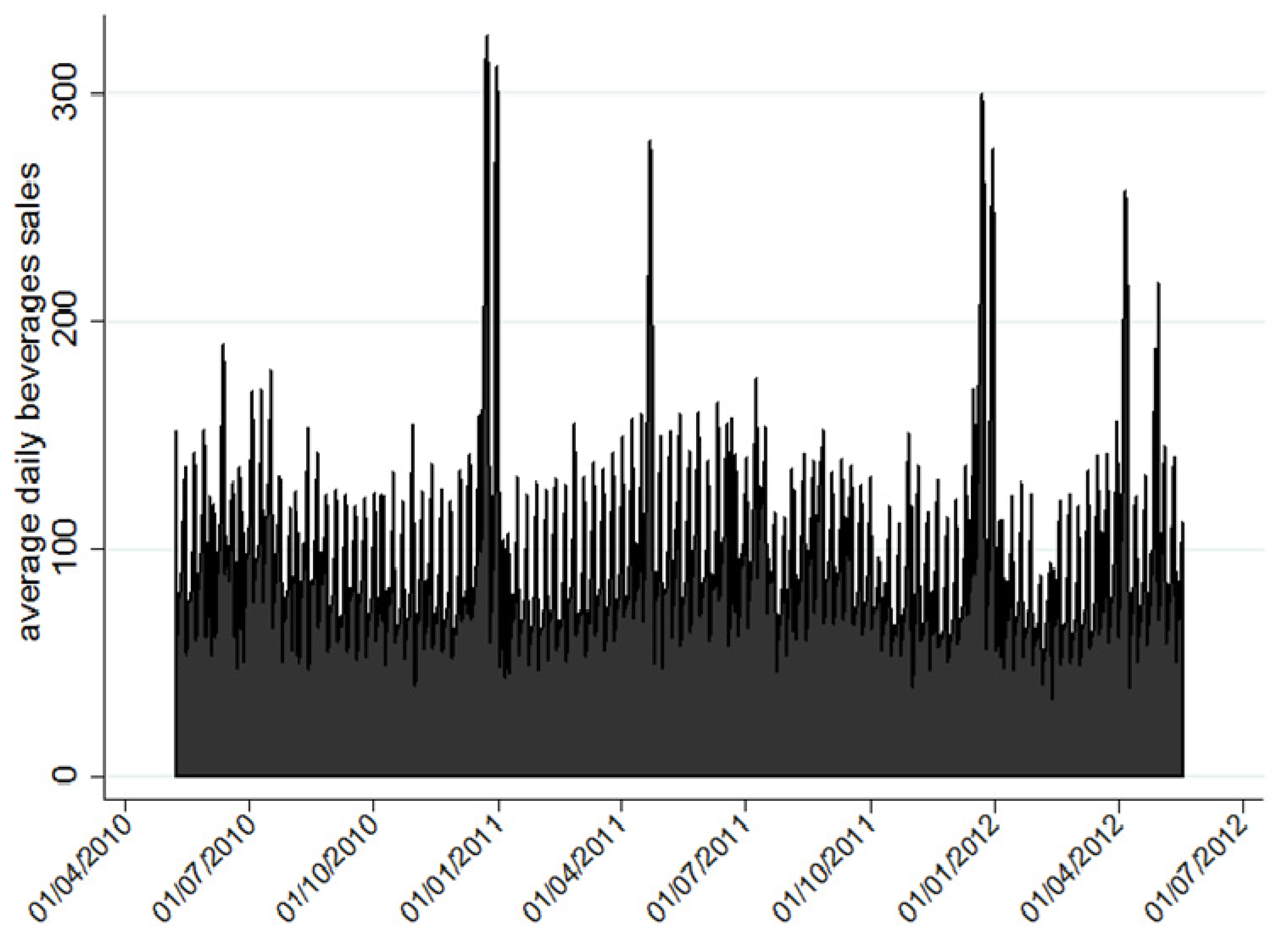
In order to minimise temporal basis risk, a covered contract period should be characterised by high weather-sales correlation. Beverage sales show seasonal patterns with booms during summer season and peaks during holidays (Figure 1). Thus, performance of weather derivatives over summer periods will be studied (May through September).

Analysing the Pearson correlation coefficients between average daily beverage sales and average daily temperatures by months (

Table 1. Correlation between average daily beverage sales and average daily temperatures, by month.

	Jan.	Feb.	Mar.	Apr.	May	Jun.	Jul.	Aug.	Sep.	Oct.	Nov.	Dec.
Pearson corr. coef.	0.0559	0.1312	0.1470	0.3280	0.1740	0.1738	0.2890	0.2225	0.1891	0.0502	0.0693	−0.0653

), it is noticeable that temperature-sales correlation is not constant throughout the year, and that it is three times stronger in summer (May to September) than in winter months (November to March)—0.21 to 0.07 on average, respectively. April and October are excluded from the correlation analysis, as they are shoulder months.

In order to allow for weather sensitivity to differ between months, which is an economically reasonable assumption, monthly specific weather derivative contracts are designed for May, June, July, August and September, instead of one overall seasonal contract for summer. In this way, retail managers can design customised weather risk management solutions specific to each month, thus enhancing the risk management effectiveness.

In order to define other derivative attributes, econometric models are constructed according to the model presented by Formula (1), and parameters are assessed using PCSE.

Table 2. Weather sensitivity of beverage sales, by month.

Variable	May	June	July	August	September
temp	1.224051 ***	2.6840115 ***	1.8340112 ***	2.8683797 ***	1.086543 ***
sun	−0.08842621	−0.22984299	1.0569893 **	−0.38517782	0.46564119 *
rain	0.00797104	−0.17820623	0.28424749	−0.00026603	−0.02082042
constant	28.863996 ***	9.8627568	11.66014	5.9232401	30.415982 ***
χ2	2482.7234	943.405442	1244.4146	1745.3798	2238.4623
df	19	20	16	20	16
N	3792	3020	3110	3112	3084
RMSE	25.367282	29.725892	27.073215	40.516222	22.933565
R2	0.62609718	0.57975282	0.58999838	0.40536533	0.56410881

Note: * p < 0.05; ** p < 0.01; *** p < 0.001. RMSE: root mean square error; df: degrees of freedom.

gives statistical output of constructed models of weather sensitivity by month. Results concerning only weather variables are presented, while full output is available from the author upon request.

Temperature is the only weather variable with a significant impact on beverage sales in all summer months, and, since it shows the highest impact on sales, underlying weather indices are constructed as temperature indices. Indices are computed as cumulated average temperature (CAT) indices, which are customary weather indices for Europe in summer seasons. The CAT index is calculated as a simple summation of average daily temperatures during the covered period:

$$\mathrm{CAT}={\displaystyle {\displaystyle \sum }_{\mathrm{i}=1}^{\mathrm{n}}{{\displaystyle \mathrm{T}}}_{{{\displaystyle \mathrm{avg}}}_{\mathrm{i}}}},$$

(2)

$${{\displaystyle \mathrm{T}}}_{{{\displaystyle \mathrm{avg}}}_{\mathrm{i}}=\frac{{{\displaystyle \mathrm{T}}}_{\min }+{{\displaystyle \mathrm{T}}}_{\max }}{2}},$$

(3)

where i stands for day and n for number of days in a covered period. Temperature is measured in meteorological stations situated in seven cities in northwestern and central Croatia (Zagreb, Bjelovar, Čakovec, Krapina, Karlovac, Sisak and Varaždin). As a type of weather derivatives contract, performances of which are examined, options are chosen because, compared to swaps, options are a lot less risky as derivative types, so it can be hypothesised that hedgers would prefer weather options over weather swaps. More precisely, the application of put options will be assessed since beverage retailers seek protection against cooler than usual summers and low temperatures. Payoff of put options can be presented by the following formula:

$$p(x)=\max \left[0,T\times (S-W)\right]-premium,$$

(4)

where T stands for tick, S for strike and W for realised weather index during contract period. The payoff from weather options is not always positive, but can be negative as well if deviation of a realised weather index from a predetermined strike level (S − W) is smaller than the prepaid premium. However, the loss from an option can never be higher than the cost of the premium.

Strike is calculated as a 10-year average CAT index (in the period 2000 to 2009) in selected months at selected meteorological stations, as is common practice in the over-the-counter (OTC) market [42]. Some authors believe it is better to include longer weather observations, heading back 20 to 40 years, as to include more variation [55], but, given pronounced climate change, it can be argued that shorter weather observations provide more credible strike level. Prior to the calculation of strike, temperature series are tested for trends by regressing temperature values on time variables. Results indicate no trend in temperature, meaning that strike can be calculated based on original temperature values.

Tick value is determined as to reflect temperature sensitivity of beverage sales, i.e., the change in beverage sales following the 1 °C increase in average daily temperature. Statistically, tick value equals temperature regression coefficients presented in Table 2.

Premiums are calculated using a simple historical burn method as an average swap payoff over the past ten years (2000–2009) and can be defined as a fair or impartial premium because it drives the long-term option payoff to be zero, and thus privileges nor buyer nor seller. Historical burn analysis is an often-used method in literature [8,9,56]. Premiums are calculated according to the following formula:

$$\mathrm{p}(\mathrm{x})=\frac{{\displaystyle {\displaystyle \sum }_{\mathrm{i}=1}^{10}\left[{{\displaystyle \mathrm{T}}}_{\mathrm{i}}\times ({{\displaystyle \mathrm{S}}}_{\mathrm{i}}-{{\displaystyle \mathrm{W}}}_{\mathrm{i}})\right]}}{10}$$

(5)

where i stands for each year in a preceding 10-year period from 2000 to 2009, T for tick, S for strike, and W for realised weather index during the covered period.

From each of the seven cities in which temperature is measured, one food store is randomly selected for which five temperature put options are created for each month of the summer season. As a result, a total of 35 temperature put options are created, performances of which are analysed.

Table 3. Attributes of designed weather derivatives.

Attribute	Contract period
	May	June	July	August	September
Contract type	Put option	Put option	Put option	Put option	Put option
Meteorological element	Temperature	Temperature	Temperature	Temperature	Temperature
Weather index	CAT	CAT	CAT	CAT	CAT
Tick	1.22	2.68	1.83	2.86	1.08
Strike:
Zagreb	540	622	686	668	486
Varaždin	523	604	664	645	462
Krapina	518	602	660	638	460
Karlovac	518	605	673	647	457
Čakovec	510	596	651	632	448
Sisak	545	631	693	669	478
Bjelovar	558	635	695	674	481
Premium:
Zagreb	18.68	48.55	19.97	67.94	17.04
Varaždin	18.22	54.93	22.04	55.87	14.05
Krapina	19.14	49.57	19.68	60.75	17.10
Karlovac	22.17	51.83	20.69	58.14	18.00
Čakovec	19.22	54.48	21.21	56.88	15.26
Sisak	17.83	54.99	19.18	56.94	16.62
Bjelovar	21.20	65.55	22.35	59.21	17.22

CAT: cumulated average temperature.

summarises designed attributes of weather derivatives.

Strike is measured in the same units as weather index, in CAT degrees. Premium and tick are measured in the same units as beverage sales, in indexed points of litres per square meter. When calculating monetary effect of temperature on beverage sales, i.e., tick value in monetary units, tick value in index points should be multiplied by index point value and average price of one litre of non-alcoholic beverages.

5. Results and Discussion on Effectiveness of Weather Derivatives

The effectiveness of temperature put options is examined on simulated economic values of beverage sales if options were applied in the period from May 2010 to May 2012, and results are presented in

Table 4. Performance of temperature put options, by city and contract period.

	May	June	July	August	September
Zagreb
∆(%) in average e.v. of sales *	0.26	−2.09	−0.92	−1.66	0.06
∆(%) in standard deviation	36.14	−2.30	0.00	−38.97	−11.99
Varaždin
∆(%) in average e.v. of sales	0.57	−1.58	−0.54	−0.40	0,57
∆(%) in standard deviation	−9.97	933.84	−8.52	−62.06	−13.70
Krapina
∆(%) in average e.v. of sales	0.17	−1.05	−0.36	−0.83	−0.02
∆(%) in standard deviation	6.54	8.10	−1.57	−98.26	−7.04
Karlovac
∆(%) in average e.v. of sales	0.49	−2.38	−0.69	−1.89	−0.28
∆(%) in standard deviation	0.46	−26.69	−10.08	−45.29	−16.03
Čakovec
∆(%) in average e.v. of sales	0.51	−1.87	−0.44	−0.99	0.32
∆(%) in standard deviation	−17.44	82.45	−5.92	−47.94	−37.94
Sisak
∆(%) in average e.v. of sales	0.92	−1.46	−0.62	−1.06	0.04
∆(%) in standard deviation	1.20	−34.02	−7.35	−19.80	−20.32
Bjelovar
∆(%) in average e.v. of sales	1.71	−1.71	−0.63	−1.52	0.10
∆(%) in standard deviation	−12.43	−45.84	−10.68	−35.96	−12.85
Average
∆(%) in average e.v. of sales	0.66	−1.73	−0.60	−1.19	0.11
∆(%) in standard deviation	0.63	130.79	−6.30	−49.76	−17.12

* Average e.v. of sales stands for average economic value of sales, which is comprised of average beverage sales and (positive or negative) derivative payoff.

. Temperature put options are considered effective in risk mitigation if their application results in lower deviation of economic value of beverage sales. Reduction in deviation is presented by negative values. In other cases, application of temperature put options results in more volatile, i.e., more uncertain economic value of beverage sales and is considered ineffective. Values in bold reflect the month for a given city, in which usage of temperature put options results in the largest reduction in deviation of economic value of beverage sales.

Results show that effectiveness of temperature put options in reduction of volatility of economic value of sales for studied food stores varies by month and city, and ranges from 1.6% (for Krapina in July) to 98.3% (for Krapina in August). For a given city, effective application of weather options ranges from three to five months. Out of a total of 35 temperature put options that are designed, the application of 27 of them shows reduction in sales deviation, which results in a high effectiveness rate of 77% for the entire store sample. On average, temperature put options prove to be effective in July, August and September. The largest reduction in volatility of economic value of beverage sales is realised in August, which is the month with the strongest impact of temperature on sales and historically the most volatile temperature.

On average, in July and August, the lower level of volatility is achieved at the lower level of average economic value of beverage sales, which reflects the trade-off between return and risk of investment that a retailer must make. Application of temperature put options in September results in lower volatility at a higher level of average economic value of beverage sales, providing twofold benefits for potential end-users. It is likely that retailers with high aversion towards risk and uncertainty will choose to cover sales in August, and are willing to give up some sales in exchange for a large reduction in uncertainty of sales revenue. On the other hand, the use of temperature put options in June proves highly ineffective. Given that options in June result in lower average sales and higher volatility, their application on average seems highly unlikely. With Varaždin excluded from calculation, their application turns effective with a slight reduction of sales volatility of 3%. The incredibly high value of standard deviation change in June in Varaždin is due to warm June temperatures in 2011, which resulted in a single negative derivative payoff and hence high standard deviation altogether. The month of May stands out because application of temperature put options results, on average, in a slight increase in volatility, as well as average economic value of beverage sales. Accordingly, May options are ineffective in terms of weather risk mitigation and are unacceptable for hedgers. However, May options seem appealing for retailers who are willing to take more risk in exchange for a higher return.

Results regarding risk reducing performance of temperature put options in retail are comparable to effectiveness of weather derivatives in other industries. Application of weather derivatives results in volatility reduction in crop production ranging from 16% to 77% [43], 80% in golf tourism [41], and 20% in viticulture [8].

The cost of the premium is a key determinant of temperature put option performance. High premiums are a result of large average option payoffs during the historic period, so it can be expected that a given option will result in large average payoffs in the near future as well.

Table 5. Cost of premium relative to maximum weather derivative payoff.

Premium (%)	May	June	July	August	September	Average
Zagreb options	18.62	25.55	28.28	28.70	28.55	25.94
Varaždin options	17.68	31.25	26.48	25.12	26.90	25.49
Krapina options	17.55	29.49	20.75	23.46	29.74	24.20
Karlovac options	19.17	34.76	27.82	26.13	44.50	30.48
Čakovec options	17.78	33.31	25.46	24.76	25.37	25.34
Sisak options	18.53	30.05	31.32	24.67	38.54	28.62
Bjelovar options	25.92	34.35	33.70	23.95	25.31	28.65
Average	19.32	31.25	27.69	25.26	31.27	26.96

presents premiums of designed options expressed, relatively, as percentages of maximum payoffs during the previous 10-year period.

Premiums of designed options for food retail stores are relatively high, ranging from 17.6% to 44.5% of maximum payoffs. These results are consistent with results in agriculture. Vedenov and Barnett [43] reports that the cost of option premiums in crop production ranges from 17.3% to 45.2% of the maximum payoff. Generally, it can be concluded that weather options with higher premiums result in larger reduction in the volatility of the economic value of beverage sales, but exceptions do exist.

The obtained results offer important implications for both academics and professionals. Future research should study the effectiveness of different types of weather derivative contracts—for example, swaps. Studies on weather derivative effectiveness should also be performed in other climatic regions and retail stores with different assortment in order to give more comprehensive insights on weather derivatives performance in retail.

6. Conclusions

Prior to the advent of weather derivatives, companies had limited solutions for non-catastrophic weather risk management. Many companies simply ignored the weather risk or were trying to cope with the consequences of adverse weather to the best of their abilities. Nowadays, the weather risk management principles are more necessary due to the omnipresent economic crisis and increased weather volatility caused by climate change. In the short run, some of the adverse weather effects can be mitigated by weather forecasts and adequate preventive measures, while, in the long run, weather cannot be predicted with validity adequate for business decision-making, and solutions that provide indemnity are needed. Weather derivatives provide flexible weather risk management solutions with completely objective payoffs, thus minimising moral hazard and adverse selection problems.

Given that derivatives allow for speculations that are often associated with negative connotations, especially in developing countries, weather derivatives are often perceived as highly risky investments that presents massive obstacles in their application. This is why weather derivatives should be presented and commercialised among potential users in the form of weather index insurance. By doing so, insurance companies could come to the fore as major sellers of weather derivatives, thus enabling the application of such sophisticated weather risk management solutions in developing countries that do not have organised futures markets.

Based on the empirical data, temperature put options are designed for food retailers as risk mitigating tools against adverse temperature impact on beverage sales during summer season. Options are designed to cover each of the five months and seven cities, which resulted in a total of 35 temperature put options. Their effectiveness is assessed based on the reduction in volatility of expected economic value of beverage sales. Results show that performance of temperature put options differs between months and cities. On average, temperature put options prove to be effective in July, August and September, providing a reduction of sales volatility in the range of 1.6% to 98.3%. When deciding which period to cover with weather derivatives, retailers need to take into account sales sensitivity to weather and average historic volatility of the weather index. The final results of weather derivative application depend on the specific weather conditions during the contract period.

Scientific contribution of this article is reflected in the studying of an insufficiently studied area and creating new knowledge on non-catastrophic weather risk management, in retail and in general. The value of the empirical research is in the econometric analysis, since only a small number of studies have quantitatively analysed the impact of weather on retail sales. The proposed method of weather sensitivity analysis can be generally applicable in other weather-sensitive industries as well. Practical value of this paper is reflected in the broadening of the potential areas of weather derivative application, both in new industries and in emerging markets. To the author’s knowledge, this is the first paper that studies the effectiveness of weather derivative application in food retail based on the econometrical weather sensitivity analysis. Additional value of this paper is that it illustrates the design process of customised weather derivatives based on the empirical data. Methodologically, the study distinguishes because two dimensions of data are observed, which calls for application of panel analysis and provides more precise results on weather sensitivity and weather derivative effectiveness.

Further research on weather sensitivity of retail sales is needed in order to provide more comprehensive insights on weather risk in retail. Future research should explore weather sensitivity of different product categories and different store formats, as well as weather derivative effectiveness in reducing volatility of its sales. It would be also interesting to design weather derivatives with alternative attributes and compare the effectiveness of such alternative weather derivative designs; for example, weather derivatives with limited payoffs, different covered periods, different strike levels, and, consequentially, different premiums. In the future, weather sensitivity of sales could be tested with nonlinear models as well as model fit on out-of-sample data.