Article

Bank Credit Risk Management and Rating Migration Analysis on the Business Cycle

1
Shipping, Trade & Transport Department, Business School, University of Aegean, Chios 82100, Greece
2
Audencia Nantes School of Management, Nantes Cedex 3 44312, France
*
Author to whom correspondence should be addressed.
Int. J. Financial Stud. 2014, 2(1), 122-143; https://doi.org/10.3390/ijfs2010122
Submission received: 6 November 2013 / Revised: 11 February 2014 / Accepted: 15 February 2014 / Published: 3 March 2014
(This article belongs to the Special Issue Credit Risk under Moral Hazard)

Abstract

:
Credit risk measurement remains a critical field of top priority in banking finance, directly implicated in the recent global financial crisis. This paper examines the dynamic linkages between credit risk migration due to rating shifts and prevailing macroeconomic conditions, reflected in alternative business cycle states. An innovative empirical methodology applies to bank internal rating data, under different economic scenarios and investigates the implications of credit risk quality shifts for risk rating transition matrices. The empirical findings are useful and critical for banks to align to Basel guidelines in relation to core capital requirements and risk-weighted assets in the underlying loan portfolio.
JEL Classifications:
C15; C58; E02; E32; G21

1. Introduction

Credit risk is defined as “the potential that a bank borrower or counterparty will fail to meet its obligations in accordance with agreed terms” by the Basel Committee on Banking Supervision [1]. Credit risk is usually conceived in loan exposures and interest-generating securities which are core revenue sources for financial institutions. In an environment of global financial crisis and economic recession, banks are now increasingly exposed to credit risk from a diversity of financial instruments other than loans, including interbank transactions, trade financing, foreign exchange transactions, financial futures, swaps, bonds, equities and options, inter alia.
According to Basel II and III guidelines, banks are allowed to incorporate their own estimates of different risk exposures, adopting internal risk rating systems, in order to realistically assess their regulatory capital requirements, known as the “internal-ratings-based” (IRB) approach. Only banks meeting certain minimum conditions, disclosure requirements and approval from their national supervisor are allowed to apply this approach [2]. Furthermore, the notion of “incremental risk charge” (IRC) requires banks to calculate a one-year 99.9% VaR (value-at-risk) for losses associated with credit sensitive products in the trading book [3]. In this dynamic process, banks need to monitor credit rating shifts and potential defaults in a volatile economic environment [4].
In a broader context, the assignment process of credit risk rating takes into account both qualitative and quantitative elements ([5,6,7], inter alia). An important feature of external agency ratings is that, assuming time-homogeneity, they are assigned typically with a “through-the-cycle” (TTC; also, “stressed ratings”) approach, based on an undefined long-term perspective on credit risk but of a more stable perspective [8]. This implies an evaluation of the borrower based on a downside scenario (e.g., the worst phase in the macroeconomic cycle) rather than on current market conditions, as in the so-called “point-in-time” (PIT) approach [9,10]. TTC ratings, therefore, tend to be more stable than PIT ratings, as rating transitions (migrations)—i.e., movements from one rating class to another—are less frequent. Also, historical default rates for each rating class may be more unstable, since in bad years the default rate may increase without companies being moved to a different rating class, as occurs under the PIT approach. Since PIT ratings are sensitive to cyclical changes in the borrower’s credit risk, risk levels and corresponding capital requirements tend to increase during recession periods and to decline during economic expansions. Because of increasing (regulatory) capital requirements during downturns, banks tend to restrict lending activities or to increase price margins, both reducing funding opportunities. The economic downturn may be exacerbated by reduced funding due to increasing capital requirements from PIT rating systems and this phenomenon is referred to as procyclicality. Empirical evidence suggests already that banks, for a number of reasons, reduce lending more than the reduction of economic activity during downturn. Therefore, procyclicality has been a critical issue in Basel II and II capital guideline rules that clearly advise TTC ratings. Rating stability, on the other hand, may be in conflict and not reflect recent changes in default risk, as ratings are adapted slowly to these changes. Many of the internal rating systems built by financial institutions are PIT systems measuring credit risk taking into account the current conditions and situation of a borrower [6,7].
To this end, credit ratings facilitate bank evaluation of borrower’s credit quality and worthiness. Credit rating (or scoring) transition, in specific, is the migration of a debt instrument from one rating to another rating over a period of time. This migration is the movement either as an upgrade or a downgrade from an existing rating and indicates the change in the credit quality of an entire loan portfolio as well as the potential for significant financial stress and loan default [11]. In relation to that, transition matrices represent a key tool when assessing the riskiness of a credit exposure. A transition matrix reports the distribution of issuers/borrowers based on their initial rating class (on rows) and on their final status (in columns: final rating class, withdrawn rating or default) at the end of a particular time interval (e.g., one-quarter or one-year). It is now widely recognized that the implementation of a transition analysis approach would support banks to accurately model credit rating migration probabilities 1 as an integral part of modern credit risk management [12]. Indeed, the recent turmoil in global capital markets and the adverse prevailing economic conditions have resulted in a widespread shift towards negative credit ratings, signalling severe deterioration in credit quality. Credit risk transitions are seen to exhibit different behavioural patterns over different macroeconomic phases and business cycle states (booms–contractions). To take into account the implication of business cycles and real economic activity on credit risk and rating migration behaviour, a number of studies distinguish between different economic phases (regimes), treating booms separately from contractions ([13,14,15,16,17], inter alia).
The core objective of the paper contributes to the empirical investigation of credit risk transition patterns in different business cycle states. More specifically, the study attempts to model corporate rating migration probabilities on bank loan portfolios, incorporating the state of real economic activity as well. The empirical approach assumes an IRB bank internal rating framework. The paper proceeds as follows. Section 2 reviews past empirical literature on critical factors that arguably influence bank loan portfolio monitoring as well as the assessment of borrowers’ creditworthiness. Section 3 proposes and applies a discrete-time maximum likelihood (DTML) model [18,19,20] and incorporates key macroeconomic factors to reflect different states of the real economy. Section 4 evaluates the empirical findings on the basis of a bank’s internal rating system and, finally, Section 5 concludes.

2. Literature Review

As BCBS postulates “borrowers and facilities must have their ratings refreshed at least on an annual basis; certain credits, especially higher risk borrowers or problem exposures, must be subject to more frequent review. In addition, banks must initiate a new rating if material information on the borrower or facility comes to light” [21]. BCBS, furthermore, indicates that monitoring shifts in new rating patterns can be a useful input in anticipating future default signals, when scrutinising obligors’ historical track records. Such monitoring can be founded upon the notion that phases of increased default risk are seen to follow earlier phases of highly frequent new ratings. Nevertheless, a bank’s feasibility to continuously monitor a risky borrower and to efficiently assess the level of creditworthiness remains a critical issue.
Past relevant studies have dealt with credit rating migration analysis taking into consideration the following issues. In case a sequence follows a first-order Markov process, the migration probability matrix can be critical in revealing transition properties. This outcome, however, may be biased towards the dependence of immediately successive events and does not contain all prior events [22,23]. The type on dependence is often known as the “memory of the process”, which in this case has a length of one-step (distance between adjacent events). Furthermore, whenever one-step transition probabilities do not depend on time, so that Ijfs 02 00122 i001, they are assumed to be stationary and the Markov chain is also stationary or time-homogeneous [24]. Finally, key macroeconomic factors are argued to be critical inputs to be incorporated in the modeling process, in order to proxy business cycles and states of the economy.

2.1. First-Order Markov Process

Transition matrices are at the centre of modern credit risk management. A standard specification for rating transition probabilities is the first-order, time-homogeneous Markov model, which is based on the assumptions that (a) the probability of migrating from one rating class to another depends on the current rating only and (b) the probability of changing from one rating class at time t to another class at time t + n does not depend on t. Past empirical evidence, nevertheless, indicates that transition probabilities are influenced by rating history (see: [25,26,27]). Consecutive rating changes in the same direction are seen to be more frequent than in the opposite direction. Since the effect is stronger in the case of downgrades, this phenomenon is referred to as “downward momentum” [28].
A number of studies postulate that credit ratings under the first-order Markov assumption provide a reasonable practical approximation, as long as different transition matrices are considered in booms from contraction states [15,26,29,30]. Markovian models are seen to produce information on the probabilities of rare transitions (compared with a typical multinomial or cohort approach), even in case these transitions are not actually observed in the data [27]. The state space of the rating process can expand to render the Markov assumption reasonable. Furthermore, a Markovian model can be conveniently specified for firms that are downgraded and enter, subsequently, an “excited state” for a stochastic time-horizon [27,31]. A company’s rating is termed as “excited” (“non-excited”) in case the last rating change was a downgrade (otherwise).

2.2. Time-Homogeneity

The cross-sectional and temporal homogeneity of transition intensities is critical for deriving the modeling approach to transition matrices. A number of past studies investigate transition probabilities functions of distance points in time between different rates and study whether the same transition matrix can be used for each-point-in time (PIT) independently of the date points in time. Some studies conclude that credit rating transitions can be adequately modeled as a Markov chain for typical forecast horizons (one or two years), based on in-sample datasets [32,33]. Furthermore, heterogeneity in default probability, measured by a credit rating scoring for instance, is shown to be of critical importance in affecting the shape of the loss distribution [34,35].
Several studies specify non-homogeneous models that incorporate the notion of cyclicality and treat credit rating migrations as a non-memory-less process [35,36,37]. Nickell et al. [38], for instance, investigate the dependence of ratings transition probabilities on industry, country and stage of the business cycle and argue that the business cycle dimension is critical in explaining variations in transition probabilities. Bangia et al. [15] distinguish between transition matrices dependent on the business cycle and find that the loss distribution and economic capital of a synthetic bond portfolio can vary considerably in different economic environments. Jafry and Schuermann [39] propose a “mobility-metric” (a measure of overall mobility for a rated issuer), estimated as the average of the singular values of the mobility matrix for the issuer’s profile. Similarly, Truck and Rachev [40] conclude that migration matrices estimated at different business cycle points produce significantly different VaR measures for an underlying portfolio.
When modeling credit rating migration over a specific time-horizon (not in infinity), time-homogeneity is a key issue. Modeling rating transition as a Markov chain process implies that default is considered to be an absorbing state, that is, in the long-term all assets are in default. Past studies based on external rating data and up to two-year forecasts, postulate that credit rating dynamics can be adequately modeled as a Markov chain [32,41]. Furthermore, the incorporation of discrete-time approaches rather than of continuous-time duration models with time-homogeneity is argued to be ambivalent in terms of loss efficiency in cohort data analysis. Different estimation approaches can result to large differences in portfolio risk profile and capital requirements. Estimations based on continuous-time duration settings are found to be more efficient relative to multinomial cohort based approaches [42,43].

2.3. Macroeconomic Factors

A number of studies incorporate critical macroeconomic explanatory factors and business cycle states in modeling rating transition probabilities, in order to establish linkages between underlying economic conditions and credit risk migration. Transition probabilities are seen to depend on industry, company, location and business cycle states [15,38,44,45]. Average time-to-default is found to decrease when economic activity decreases [46,47,48,49]. The time-varying cyclical nature of default rates over long historical periods has been also investigated [50,51,52].
Jafry and Schuermann [39] develop a metric that applies to migration matrices, in order to compare different estimation methods of migration probabilities. Similarly, Truck and Rachev [53] propose a class of “directed difference indices” to apply on transition matrices and these measures exhibit high correlation with differences in credit VaRs. To better understand the economic structure of time dependence, Parnes [35] examines shifts in key macroeconomic business conditions, incorporating a scaled GDP variable, contraction—expansion states and the CBOE volatility index (VIX). A number of studies test models of rating transitions in a calendar time framework over discrete time slots [36,54,55]. GDP is seen to be a key macroeconomic variable [56,57]. Recent studies incorporate alternative models in a dynamic framework, such as generalized linear mixed models (GLMM) and Markov chain Monte Carlo (MCMC) techniques [36,37] or conclude asymmetry in credit cycle dynamics [58]. Macroeconomic factors are found to affect the persistence of a low default regime more than a high default regime, supporting correlations of credit and business cycles. On the other hand, credit portfolio models conditional only upon business cycle proxies may miss out on a significant part of systematic portfolio credit risk.

3. The Discrete-Time Maximum Likelihood Framework

Α model of discrete-time maximum likelihood (DTML) is now discussed (quarterly intervals); it incorporates a parametric approach to account for the state of the economy by including key macroeconomic factors. The framework applied here is suitable for producing maximum likelihood (ML) estimates, whenever the exact time of movement between rating classes and the class occupancy between observation times are unknown; it also takes into account that the inter-examination periods (time-spans between successive ratings) may vary for different firms or individual borrowers.

3.1. Time-Homogeneity in Transition Probabilities

Initially, certain critical differences between discrete and continuous-time frameworks are discussed. For that, a first-order time-homogenous Markov chain X(t) is incorporated to indicate credit rating categories at time t (t ≥ 0). Assuming discrete data and identical observation times equally spaced for each borrower in the Markov chain (to < t1 < tj < … < tjn), such that Sj = tjtj−1 = S, for all j = 1,…, jn monitoring steps, the ML estimator of the stationary transition probabilities drawn by Equation (1) is the cohort estimator:
Ijfs 02 00122 i002
where 1, 2, …, lD are finite numbers of the Markov chain states (1, 2,…, lD−1 correspond to decreasing levels of creditworthiness and lD indicates default); P(s) denotes the lD × lD transition probability matrix with its (ll’)th element, namely pll’(s), corresponding to migration probability from state l to l’ within a s-length time interval; Nll’ = Ijfs 02 00122 i003 
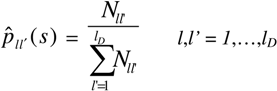
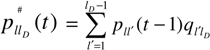
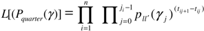
is the total number of verified transitions from l to l’.
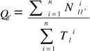
In case that observation time points are not identical and equally spaced, the cohort estimator remains “poor” as it does not correspond to the ML estimator of pll’(s) any longer, due to the fact that only the observations with identical and equal monitoring steps are considered. In other words, the cohort approach estimates the migration probabilities as observations running from the beginning to the end of a time period under study (any observations within this period interval are ignored). On the contrary, the DTML framework provides an alternative approach that contains this latter flaw.
In the continuous-time maximum likelihood (CTML) framework, the Markov chain applies transition intensities qll’(t,s) = qll’, whereby, given that state l enters in time t and is still occupied at t + s, then the transition out of l is determined by a set of lD−1 transition intensities qll’ > 0. (The intensity, qij(t), from state i to state j can be perceived as the rate of change of the probability Pij in a very short time interval, Δt). Given a time-homogenous Markov chain, the relationship between an (lD × lD) intensity matrix 2, Q, and the transition matrix, P(s), is given by Equation (2):
P(s) = eQs
In this case, the ML estimator of the transition intensity is given by Equation (3):
Ijfs 02 00122 i004
where Ijfs 02 00122 i005 denotes the number of ll’ transitions made by an obligor i and Ijfs 02 00122 i006 is the overall time that obligor i has spent in class l [26]. This is the duration estimator which counts every rating drift in a given period divided by the total time spent in each rating class. With no information available about the timing of events between observation times or about the exact transition time, neither the numerator nor the denominator of Equation (3) can be calculated [30]. Assuming discrete data (observations corresponding to a sequence of discrete time points), the duration intensities cannot be used to evaluate the transition intensities; moreover, the observation times must be identical and equally spaced, in order for the cohort estimator (Equation (1)) to provide ML estimations.
Based on earlier empirical studies [30,60,61,62] proposes a model to produce ML estimates of the intensity matrix, Q. Observation time points are assumed to be arbitrary and the exact times of rating class transitions and the class occupancy between observation times are assumed to be unknown. Transition probabilities, pll’, are expressed in terms of intensities; hence, it is vector θ of intensities qll’ to be estimated. Incorporating a canonical decomposition and assuming that Q(θ) has distinct eigenvalues, Ijfs 02 00122 i007, Equation (2) develops into Equation (4):
Ijfs 02 00122 i008
where A0 is a lD × lD matrix whose lth column is the right eigenvector for λl. The individual contribution to the total likelihood function that is to be maximized is divided into observations of the firms defaulting during the observed time ti0 = 0,ti1,…, Ijfs 02 00122 i009 
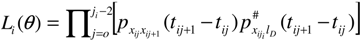
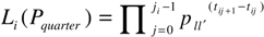
with the rating of firm i as xi0,xi1,…, Ijfs 02 00122 i010 respectively [x ∊{l,…,lD}] and those that are censored at the end of the observation time period.
Assuming that the exact time of default is known but the rating class before the default is not known, the censored observations (in the set R = {l,…,lD − 1}) contributes to the likelihood function by:
Ijfs 02 00122 i011
where for l = 1,…, lD−1
Ijfs 02 00122 i012
The non-censored observations (firms i entering default during the observed period tij) contribute to the likelihood function by:
Ijfs 02 00122 i013
where, for l = 1,…,lD−1
Ijfs 02 00122 i014
The total likelihood function is the product of the likelihood contributions over all n firms, conditional upon the distribution of firms among the states at ti0 [30]:
Ijfs 02 00122 i015
Considering the discrete-time framework (quarterly intervals), by transforming Equation (2):
Ijfs 02 00122 i016
where n = 1, …, m quarters and Pquarter is the one-quarter transition matrix.
The total likelihood function is the outcome of the likelihood contribution over firm i, as in Equation (11):
Ijfs 02 00122 i017
where pll’ = Pquarter(l,l’). Equation (11) can be rewritten as in Equation (12):
Ijfs 02 00122 i018
Thus, the log-likelihood function is given in Equation (13) as:
Ijfs 02 00122 i019
Equation (13) indicates that the quarterly transition matrix is evaluated within every observation available, where only the exact time of default is known but the previous rating class (prior to default) is unknown. Hence, an attractive feature of DTML against CTML relates to the issue that the former approach does not require iterative eigenvalue calculations to produce an outcome. In order to obtain a ML outcome in the general case of lD≥2, a Quasi-Newton algorithm with finite differences can apply to produce numerical derivatives approximations [59]. Since the algorithm is an iterative process, a starting point can be the cohort estimator [30].

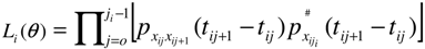
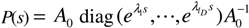
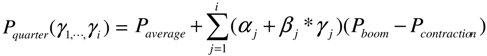
3.2. Business Cycles in Transition Probabilities

The incorporation of business cycles and the state of the economy into a time-homogenous Markov chain in a DTML framework is now discussed. As past studies postulate, the approach to estimate matrices conditioned on the business cycle remains a critical issue [15,22,33,63]. In brief, a migration matrix describes all possible transition probabilities given a rating scale [64], as in Equation (14):
Ijfs 02 00122 i020
where each pi,j represents the transition probability from state i to state j, if ij at time period t; the rows represent current ratings of obligors whereas the columns represent future ratings. The last row, L, represents the absorbing state of default, i.e., the probability of leaving the default state equals zero. With the highest rating in the first row, the elements below the diagonal are the probabilities for upgrades and the elements above the diagonal are the probabilities for downgrades. The upper part of the matrix also includes the Lth column which gives default probabilities for different ratings. The diagonal elements represent the probabilities for the ratings to be preserved in period t.
Two separate time-homogenous rating migration matrices can be estimated, conditioned on the boom and contraction state of the economy, respectively. The total transition matrix (estimated on all available observations) is used to construct the average transition probabilities. The transition matrix is anticipated to shift between upward or downward market phases, depicted by the explanatory macroeconomic variables (such as GDP per capita; GDP growth; inflation rate; external debt/exports, fiscal/external balance; [65]). In order to depict the statistical correlation between macroeconomic variables and transition matrices on the state of economy, Equation (15) is set as:
Pquarter(γ) = Paverage + (α + β * γ)(PboomPcontraction)
where γ is a key macroeconomic factor and α and β reflect the boom and contraction coefficients, respectively. In accordance with Equation (12), the log-likelihood function can be set as in Equation (16):
Ijfs 02 00122 i021
where pll’(γj)(tij+1tij) is the ll’th element of:
Ijfs 02 00122 i022
where γj is the macroeconomic variable at time tij.
In case of inclusion of i economic variables, Equation (15) can be transformed into Equation (17):
Ijfs 02 00122 i023
A number of past studies examine the issue of business cycles and states of the economy in the context of credit risk [15,17,18,22,33,38,39,42]. Some approaches classify the states of the economy as finite regimes and assume transition matrices change over time with the states of the economy. According to Xing et al. [66], this ignores the fact that the states of the economy at different periods might be different even if they are in the same regime. From this perspective, it would be better not to restrict the number of regimes. In their study, they assume the state of the economy to be continuous, and model the structural changes in the economy as the shifts of the state of the economy in a continuous space. This implies that the generators of the rating transition matrices are constant between two adjacent structural changes in the economy. Xing et al. [66] show that the generator and transition matrices of rating transitions are indeed changing over time and the estimated structural breaks are not only statistically significant but economically meaningful as well. They also demonstrate that the generator or transition matrices in different industry categories have different behaviors and, specifically, industry sectors related to finance services are more susceptible to economic changes than other sectors.

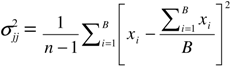
3.3. Statistical Measurements

Past studies incorporate a variety of statistical approaches, models and measurements to deal with the empirical analysis of rating migration matrices. The next sections discuss briefly the singular value decomposition metric and bootstrapping approaches. The latter are frequently incorporated in transition matrix analysis, as they arguably bear attractive properties and flexibility [42].

3.3.1. Singular Value Decomposition Metric

The singular value decomposition (SVD) is a generalization of the eigen-decomposition which can be used to analyze rectangular matrices. The main idea of the SVD is to decompose a rectangular matrix into three simple matrices: two orthogonal matrices and one diagonal matrix. Because it gives a least square estimate of a given matrix by lower rank matrix of same dimensions, the SVD is equivalent to principal component analysis (PCA) and metric multidimensional scaling (MDS) and is, therefore, an essential tool for multivariate analysis [67]. In the context of transition matrices, Jafry and Schuermann [39] propose a new metric for comparing these matrices—a mobility index—termed the “the singular value of decomposition metric”, MSVD, which has an intuitively-appealing “size” related to the average probability of migration of the original matrix. This metric for a transition probability matrix, P, of dimension lD × lD is given in Equation (18) as:
Ijfs 02 00122 i024
where the identity matrix of the same I and λj(G) denotes the jth eigenvalue of a lD × lD matrix G. By subtracting the identity matrix I from the migration matrix, only the dynamic part of the original matrix remains, reflecting the magnitude of P in terms of implied mobility. The value of MSVD is shown to indicate the “average amount of migration” contained in P; the larger the MSVD value, the higher the average probability of rating change. The distance metric between the migration matrices PI and PII, is given as in Equation (19):
ΔMSVD(PI,PII) = MSVD(PI) − MSVD(PII)

3.3.2. Bootstrap Method

The bootstrap procedure involves choosing random samples with replacement from a data set and analyzing each sample in the same way, with each observation selected separately in random from the original dataset [68]. A particular data point from the original data set could appear multiple times in a given bootstrap sample. The number of elements in each bootstrap sample equals the number of elements in the original data set. An important advantage of bootstrap against other methods is that the researcher does not need to have a preconceived notion of the original sample distribution [42]. A number of past studies [39,69] indicate that 200 and 1000 bootstrap replications are sufficient for obtaining standard errors of bootstrapped statistics and confidence intervals, respectively. On the basis of data input constraints and in line with standard earlier practice, this study assumes the number of B = 1000 replications to be sufficient.
The bootstrap approach applied in this study involves the following steps: first, selection of a number of firms in random out of the sample under study along with their rating histories; subsequent replacement until the number of firms is the same as in the original sample; second, incorporation of a cohort and a DTML estimation approach; third, repetition (B-1) times of the two previous steps, with computation of the comparative metric MSVD for every estimation, along with the confidence interval of α magnitude; α is obtained by sorting the comparative metrics in descending order and examining the breakpoints of top and bottom (1−α)/2 percentiles. The standard deviation of the transition probabilities is calculated as:
Ijfs 02 00122 i025

4. Empirical Application

The dataset of the study is based on the entire loan portfolio and internal rating system of a major Austrian bank (anonymity preserved for confidentiality reasons). An initial empirical step relates to defining the segmentation of business sectors; this is based on the respective Standard & Poor’s (S&P) segregation, including: financial institutions; insurance; consumer/services; energy and national resources; real estate; leisure time/media; and transportation. Critical issues include also the specification of a rating system with credit quality classes, grades and probabilities of migration from one class to another over the credit risk horizon. Rating agencies, such as Moody’s [70], Fitch Ratings [71] and Standard & Poor’s [72], for instance, incorporate a 21-, 20-, and a 17-grade scale, respectively, for corporate borrowers.
Past studies on internal rating systems [73], conclude a 5-grade rating system for the median bank out of the 50 largest US banking organizations. Other studies [30,56] use a 6-grade and a 7-grade rating system, respectively. A number of banks are interested in increasing the number of internal grades, either through the addition of ± modifiers or by splitting riskier grades. For the purposes of this study, a simple 5-grade rating system is constructed, with grade 1 denoting the worst (lowest) credit grade and grade 5 the best (highest) credit grade, respectively.
A critical step relates to the specification of the risk horizon. The study sample includes both large and “small and medium-sized enterprise” (SME) obligors with an annual turnover of at least €2.5 million and firms originating from a diversity of business sectors and countries of origin. These borrowers are classified according to their rating history over a 10-year horizon. The rating history of all borrowers (not defaulted by that year-end) in the reference (data-provider) bank’s loan portfolio is obtained, as of 31 December 2008. In addition, rating information for all borrowers that defaulted during 1995–2008 is collected. Legal bankruptcy proceedings and loan loss provisions are used as proxies for default. The observation period is eventually restricted to 1998–2008, in order to avoid survivorship bias and to overcome information constraints.
The dataset contains initially 210,000 observations on 51,000 borrowers, at quarterly intervals [17,58]. Subsequent to a careful data cleansing process, the dataset finally comes down to 185,000 observations on 48,000 firms. A thorough evaluation is normally conducted by the bank once a year (on a year-on-year basis as to the initial obligor’s rating).

4.1. Macroeconomics and States of the Economy

Following the initial discussion of Section 2.3, a critical issue relates to the selection of the most appropriate macroeconomic variable in order to depict the state of the economy, in the DTML framework. Past studies propose a variety of relevant variables correlated with default risk, such as, indicatively, real GDP growth and unemployment rate [74]; S&P500 returns [75]; and industrial capacity utilization (CUI index, that is ratio of actual output level to sustainable maximum output level [76]. For the purposes of this paper, the CUI index is selected as a convenient indicator, justified on several grounds [77]. First, it is available quarterly (contrary to annual variables). Second, it can be incorporated into a well-specified multivariate model with a minor impact on prediction error bias. Third, it is more stable over time relative to other widely used cyclical indicators.
Since the sample under study consists of heterogeneous firms that cannot be treated as a homogenous group, a single macroeconomic variable for the sample as a whole is rendered inappropriate. As a result, a smaller sample, consisting only of domestic (Austrian) firms/obligors, is finally undertaken; this results in 22,000 observations of 5000 firms (76.5% of the sub-sample exhibits an inter-examination frequency of one year; 16% of less than one year; and, 7.5% of more than one year). This sample is subsequently further divided into two sub-samples that correspond into a “boom” and a “contraction” economic state, respectively, in line with past relevant studies [17,27].
A number of studies propose different approaches in order to assess threshold values for macroeconomic variables, such as, for instance, calculation of average or median values of the factor under study; the best performing part is assumed to reflect the boom state and the worst performing part the contraction state, respectively ([54,78], inter alia). This study chooses to set the threshold value to the median. Based on that, the sub-samples in the boom and contraction states consist of approximately 5000 firms with 12,000 observations and 4000 firms with 10,000 observations, respectively.

4.2. Transition Probabilities in Time-Homogeneity

Average transition matrices in time-homogeneity for boom and contraction phases are now estimated. The estimation of a one-quarter transition matrix proceeds on the basis of the full sample of the bank loan portfolio under study, consisting of 185,000 observation pairs and targeting to maximize the log-likelihood function as stated in Equation (13). Table 1 summarizes the one-year cohort and the DTML estimation results.
The value of ΔMSVD quantifies the notion of “average amount of migration” contained in the transition probability matrix, P. The higher the value of ΔMSVD, the higher the average probability of rating changes. In this study, ΔMSVD is estimated at 0.0712 (at 1% statistical significance; standard error of less than 0.001). Past studies report transition matrices (estimated with a parametric time-homogeneous duration method for boom and contraction states) to exhibit a difference of 0.043 in MSVD [39]. Furthermore, comparisons of cohort and CTML estimations indicate the observed value of the distance metric to be equal to 0.00047 (at 5% statistical significance), [64]. Other studies estimate the MSVD difference between the two matrices at 0.042, [79].
The cohort transition matrix is seen to be significantly more diagonal-dominant (meaning that most of the probability mass resides along the diagonal) compared with the ML transition matrix, indicating that the latter matrix captures mobility (shifts) more efficiently. The two methods generate different probabilities of default. The one-year cohort estimator incorporates only yearly noted migrations and, in general, it is seen to typically underestimate default risk along all rating grades. Broadly, past studies conclude mixed empirical findings on the cohort method, indicating over- or under-estimated PDs [17,39,80]. The ML approach, on the other hand, incorporates events that occurred during the year as well as at year-end. Basel guidelines set a lower bound of 0.03% on PD estimates which may be used to compute regulatory capital [2]. Empirical evidence indicates that only the ML transition matrix is marginally below the critical bound of 0.03% (shaded transition probability cell; Table 1).
Table 1. Transition probabilities in time-homogeneity: Full sample.
From → To12345Default
Panel A: The one-year cohort transition matrix
10.969110.018210.005530.007120.000030.00000
(0.00173)(0.00152)(0.00052)(0.00023)(0.00006)(0.00000)
20.012720.937900.037230.010220.001570.00036
(0.00093)(0.00218)(0.00192)(0.00081)(0.00035)(0.00012)
30.000240.004110.951970.039250.003920.00051
(0.00004)(0.00021)(0.00083)(0.00073)(0.00027)(0.00005)
40.000240.000710.023820.954810.016610.00381
(0.00003)(0.00011)(0.00055)(0.00076)(0.00040)(0.00029)
50.000200.000060.004820.051200.924520.01920
(0.00012)(0.00004)(0.00052)(0.00240)(0.00280)(0.00156)
Default0.000000.000000.000000.000000.000001.00000
Panel B: The one-year discrete-time ML transition matrix
10.940450.046720.008330.00388 Ijfs 02 00122 i0260.00039
(0.00283)(0.00273)(0.00081)(0.00052)(0.00019)(0.00029)
20.030660.854430.081770.029930.002830.00038
(0.00188)(0.00293)(0.00239)(0.00193)(0.00039)(0.00133)
30.001220.019820.876080.095550.006110.00122
(0.00017)(0.00044)(0.00152)(0.00121)(0.00025)(0.00015)
40.000670.002610.072110.877060.041220.00633
(0.00007)(0.00002)(0.00084)(0.00249)(0.00082)(0.00018)
50.000520.000540.018830.133310.784390.06241
(0.00026)(0.00027)(0.00073)(0.00422)(0.00467)(0.00390)
Default0.000000.000000.000000.000000.000001.00000
Both transition matrices are estimated for 1998–2008. The DTML transition matrix is based on all observation pairs with an inter-examination time of less than or equal to five years. Standard errors (in parentheses) are based on a non-parametric bootstrap approach with B = 1,000 replications. The 99% confidence interval is calculated at 0.0721–0.0824 by non-parametric bootstrapping. The diagonal entries are in bold for convenience.

4.3. Transition Probabilities in Time-Dependence

Prior to investigating transition matrices in time-dependence, average transition matrices in time-homogeneity are initially estimated, on the basis of the bank loan portfolio under study, focusing only on the sub-sample of the domestic obligors. The one-year average cohort and the DTML estimations are summarized in Table 2. The ΔMSVD is estimated at 0.0912 (at 1% statistical significance; standard error of 0.006). This transition matrix displays similar characteristics as the earlier transition matrix estimated on the full sample.
Table 2. Transition probabilities in time-homogeneity: Sub-sample—domestic obligors only.
From → To12345Default
Panel A: The one-year cohort transition matrix
10.927060.037710.031120.004110.000000.00000
(0.019662)(0.01233)(0.01781)(0.00406)(0.00000)(0.00000)
20.002810.936680.046120.012730.001660.00000
(0.00199)(0.00590)(0.00441)(0.00231)(0.00088)(0.00000)
30.000440.005510.948060.041130.004820.00004
(0.00021)(0.00084)(0.00272)(0.00233)(0.00071)(0.00022)
40.000000.000220.025720.959810.013220.00103
(0.00000)(0.00021)(0.00162)(0.00217)(0.00188)(0.00044)
50.000000.000000.004920.071110.915640.00833
(0.00000)(0.00000)0.001820.007290.008330.00281
Default0.000000.000000.000000.000000.000001.00000
Panel B: The one-year discrete-time ML transition matrix
10.835810.127730.012220.023780.000420.00004
(0.02773)(0.02114)(0.00722)(0.00872)(0.00019)(0.00001)
20.006680.844580.117290.028710.002550.00019
(0.00198)(0.00626)(0.00551)(0.00277)(0.00715)(0.00002)
30.001540.016220.848380.125210.008100.00055
(0.00048)(0.00152)(0.00303)(0.00322)(0.00082)(0.00027)
40.000510.001770.082210.878830.031980.00470
(0.00021)(0.00031)(0.00372)(0.00333)(0.00278)(0.00069)
50.000050.000620.009230.133020.804870.05221
(0.00002)(0.00061)(0.00140)(0.01662)(0.01442)(0.00523)
Default0.000000.000000.000000.000000.000001.00000
Both transition matrices are estimated for 1998–2008. The DTML transition matrix is based on all observation pairs with an inter-examination time of less than or equal to five years. Standard errors (in parentheses) are based on a non-parametric bootstrap approach with B = 1000 replications. The 99% confidence interval is calculated at 0.0811–0.1466, obtained by non-parametric bootstrapping. The diagonal entries are in bold for convenience.
Table 3 summarizes the results on time-homogenous one-year transition matrices in boom and contraction phases, based on the DTML approach. The ΔMSVD is estimated at 0.0133 (at 6% statistical significance; standard error of 0.007). As indicated (shaded transition probability cells), four transition probabilities in each of the two ML-estimated transition matrices (boom and contraction phases) remain below the 0.03% bound, which satisfies relevant Basel guidelines. The probability of remaining at the lowest risk grade 1 is significantly larger in the boom than in the contraction transition matrix (by 0.05663 point). Furthermore, a higher probability of improvement in the expansionary phase is seen in grade 4 (4 → 1, 4 → 2 and 4 → 3). The other transition probabilities exhibit a wavering behavior, depending upon the business cycle state and the risk grade they correspond to. Most of transition probabilities (10 out of 15) that reflect risk-grade improvement (cells on the left of the diagonal) are higher during booms, as anticipated. Significant differences are also seen in default probabilities (all of which are found to be lower in booms). These findings support the robustness of CUI as a key macroeconomic variable to produce transition matrices in different states of the economy in the context of this study.
Table 3. Transition probabilities in time-homogeneity: Discrete-time maximum likelihood (DTML) results on business cycle states.
From → To12345Default
Panel A: The one-year ML boom transition matrix
10.849780.114430.006340.028770.00066 Ijfs 02 00122 i027
(0.02555)(0.02288)(0.00421)(0.01729)(0.00027)(0.0000)
20.005240.839840.119600.031750.00351 Ijfs 02 00122 i028
(0.00143)(0.00911)(0.00832)(0.00420)(0.00165)(0.00002)
30.000870.013320.852090.127780.00582 Ijfs 02 00122 i029
(0.00038)(0.00144)(0.00525)(0.00425)(0.00096)(0.00004)
40.000530.001770.084650.869280.042300.00147
(0.00024)(0.00048)(0.00363)(0.00488)(0.00264)(0.00049)
5 Ijfs 02 00122 i0280.001330.008430.275550.679040.03559
(0.00002)(0.00096)(0.00061)(0.01664)(0.01773)(0.00521)
Default0.000000.000000.000000.000000.000001.00000
Panel B: The one-year ML contraction transition matrix
10.793150.182230.012230.011880.00048 Ijfs 02 00122 i030
(0.03882)(0.03216)(0.008150)(0.01929)(0.00028)(0.00001)
20.007990.834150.128330.028110.00126 Ijfs 02 00122 i031
(0.00221)(0.00836)(0.00825)(0.00372)(0.00182)(0.00003)
30.001870.017220.863200.102770.013220.00172
(0.00056)(0.00177)(0.00523)(0.00449)(0.00142)(0.00033)
40.000320.000660.082800.869130.042210.00488
(0.00028)(0.00015)(0.00427)(0.00522)(0.00303)(0.00161)
5 Ijfs 02 00122 i030 Ijfs 02 00122 i0320.017220.277310.653290.05208
(0.00002)(0.00003)(0.00466)(0.01662)(0.01734)(0.00911)
Default0.000000.000000.000000.000000.000001.00000
Both transition matrices are estimated for 1998–2008. Both DTML transition matrices are based on all observation pairs with an inter-examination time of less than or equal to five years. Standard errors (in parentheses) are based on a non-parametric bootstrap approach with B = 1000 replications. The 99% confidence interval is calculated at 0.0006–0.0311, obtained by non-parametric bootstrapping. The diagonal entries are in bold for convenience.
The log-likelihood function (Equation (16)) is now implemented to determine the time-dependent one-quarter transition matrix (as in Equation (17)). All available observation pairs are incorporated to estimate α and β by maximizing Equation (16); this results into α = −5.6121 and β = 0.0641. Convenient restrictions are then set on γ, in order to ensure that that P(γ) fulfills transition matrix requirements. Thus, the range of upper and lower values γ is allowed to take runs from 69.23–89.81 percent; these values correspond to minimum and maximum values that γ has recorder historically over the study period (1998–2008). Hence, Equation (15) can be re-written as in Equation (21):
Pquarter(γ) = Paverage + (−5.6121 + 0.0641 * γ)(PexpansionPrecession)
Table 4 summarizes the empirical findings from the estimation of one-year transition matrices on different business cycle states of the economy. The γ coefficient can obtain four different values (one for every quarter of the year) that represent different economic scenarios, on the basis of quarterly observations (as in panels A to D; Table 4). Panels A and B correspond to phases of boom and contraction, respectively; panel C corresponds to transition states in the economy, namely a slump or recovery phase (in-between recession and boom phases); finally, panel D corresponds to mixed economic states, incorporating all eligible γ values and demonstrating the course of the economy on a business cycle (from boom to contraction). The largest Δ’s in ΔMSVD are obtained in a contraction scenario (as of Equation (19); at 1% statistical significance).
The default probabilities for risk-grades 1, 2, and 3 are seen to be lower in the “average state” panel than in the “mixed state” panel. More frequently, the largest part of data for defaults corresponds to risk grade 5 surpassing any other risk-grade. This implies that default transition comparisons could be restricted to the transition from risk-grade 5 to default. When comparing migration probabilities from risk-grade 5 into default in all four matrices on different business cycle scenarios, PDs increase from the lowest in the boom state, followed by the average and mixed states and ending, finally, into the highest in the contraction state. As anticipated, the worse (more unstable) the state of the economy is, the higher the respective PDs are.
Past studies argue that PDs should be preferably overestimated in boom states rather than underestimated in contraction states [39]. Default risk during contraction (boom) is statistically and economically overestimated (underestimated) by the naive cyclical approach relative to the mixture of Markov chains approach and more so for longer prediction horizons [17]. The comparison of time-homogenous and time-dependent functions in this study, during the boom state for instance, reveals that the estimated rating migration matrix in the context of the latter function displays a higher probability from risk-grade 5 to default than of the former function (0.05281 and 0.03559, respectively). This indicates that the time-dependent function overestimates PDs during boom phases. A reason for this may be that the PDs of the time-dependent contraction transition matrix (Panel B; Table 4) are higher than the time-homogenous average contraction transition matrix (Panel B; Table 3).
Table 4. Transition probabilities in time-dependence: DTML results on different business cycle scenarios.
From → To12345Default
Panel A: The one-year ML boom transition matrix
10.839870.117010.017520.025050.000510.00004
20.006110.847850.117610.025510.002760.00016
30.001770.018820.855820.116620.006230.00074
40.000630.001520.083390.879660.031190.00361
50.000050.000940.007350.299010.640470.05218
Default0.000000.000000.000000.000000.000001.00000
γi = 89.81 (i = 1, 2, 3, 4)
Panel B: The one-year ML contraction transition matrix
10.77850.177720.028810.014550.000380.00004
20.007310.842950.126730.021170.001660.00018
30.001550.017730.848860.117320.012820.00172
40.000380.007220.082210.867400.036610.00618
50.000030.000090.016620.176290.734880.07209
Default0.000000.000000.000000.000000.000001.00000
γi = 69.23 (i = 1, 2, 3, 4)
Panel C: The one-year ML average transition matrix
10.812040.144220.014420.028840.000440.00004
20.006440.820100.148020.023190.002110.00014
30.001410.016220.831440.142900.007110.00092
40.000520.001620.085180.868020.039810.00485
50.000050.000700.008520.166190.771720.05282
Default0.000000.000000.000000.000000.000001.00000
γi = 74.33 (i = 1, 2, 3, 4)
Panel D: The one-year ML mixed transition matrix
10.825240.127730.018830.027710.000440.00005
20.006410.852170.116620.021880.002750.00017
30.001770.016220.871850.100310.008510.00134
40.000570.001660.085100.875380.032870.00442
50.000040.000560.009550.177390.759500.05296
Default0.000000.000000.000000.000000.000001.00000
γ1 = 89.81; γ2 = 74.33; γ3 = 74.33; γ4 = 69.23
The DTML transition matrices are estimated for 1998–2008 and are based on all observation pairs with an inter-examination time of less than or equal to five years. The γi’s values refer to the i quarter of the year (i = 1, 2, 3, 4) and correspond to different economic scenarios and combinations of business cycle states for each quarter of the year. Panels A and B correspond to boom and contraction phases, respectively; panel C corresponds to transition states in the economy, namely a slump or recovery phase; panel D corresponds to mixed economic states, incorporating all eligible γ values and demonstrating the course of the economy on a business cycle (from boom to contraction). The diagonal entries are in bold for convenience. ΔMSVD (Boom − Contraction) = 0.01726; ΔMSVD (Average − Boom) = −0.00352; ΔMSVD (Average − Contraction) = 0.01172; ΔMSVD (Mixed − Boom) = −0.05281; ΔMSVD (Mixed − Contraction) = 0.00825; ΔMSVD (Mixed − Average) = −0.00168.
To sum up, this study contributes certain interesting and useful empirical findings to the relevant empirical literature. First, comparing different estimation methods on time-homogenous average transition probabilities, the ML transition matrix is found to have a better capture rating transition mobility relative to the more diagonal-dominant cohort estimated transition matrix. Second, the application of the DTML method to business cycle states (in order to examine time-homogenous average transition probabilities) indicates that most transition probabilities reflecting risk-grade improvement are, conceivably, higher during the boom state. Third, there appears to be significant differences in default probabilities but all of them are seen to be lower in the boom state. Forth, empirical evidence supports the robustness of CUI index as a key macroeconomic variable that can adequately contribute to transition matrices that incorporate different states in the economy. Finally, comparing probability migrations from risk-grade 5 to default in different business cycle scenarios, the DTML approach indicates that the PDs increase from the lowest in the boom state, followed by the average and mixed states and ending in the highest in the contraction state, justifying that the worse the state of the economy is, the higher the respective PDs are. The discrete-time (versus continuous-time) framework is seen to be convenient and efficient in studying credit rating migration settings.

5. Conclusions

A focal issue in Basel directives emphasizes on the intensified sensitivity banks should pay to capital requirements in correspondence to the risk exposures of the bank’s assets. In other words, the level of capital a bank should hold is to be directly related to the riskiness of its underlying assets portfolio. Nevertheless, business cycle fluctuations can exert an impact on bank capital adequacy requirements. Under Basel guidelines, banks are allowed to incorporate own estimates to critical risk parameters in order to calculate regulatory capital.
Given that regulatory measures of financial robustness (such as the Tier-1 capital ratio) refer to core bank capital and risk-weighted assets, the empirical estimation of convenient credit risk migration matrices remains a critical exercise for bank capital requirements against unexpected losses in the loan portfolio as well as for efficient risk control. This paper enriches and expands past empirical literature by examining the linkages between credit risk management and macroeconomic states. This appears to be one of the first studies to empirically estimate and compare the DTML and CTML approaches and then apply the DTML approach to four different business cycle scenarios (boom, contraction, average and mixed economic states) to produce risk transition matrices. Further empirical research in this field remains useful and timely.

Author Contributions

Dimitris Gavalas and Theodore Syriopoulos have written the paper jointly contributing to its theoretical foundations and empirical applications. This paper relates to initial output from D. Gavalas’ doctoral research, supervised by T. Syriopoulos.

Conflicts of Interest

The authors declare no conflict of interest.

References

  1. Basel Committee on Banking Supervision (BCBS). Principles for the Management of Credit Risk. Basel, Switzerland: Bank for International Settlements, 2000. [Google Scholar]
  2. Basel Committee on Banking Supervision (BCBS). International Convergence of Capital Measurement and Capital Standards: A Revised Framework. Basel, Switzerland: Bank for International Settlements and Basel Committee on Banking Supervision Publications, 2004. [Google Scholar]
  3. Basel Committee on Banking Supervision (BCBS). Guidelines for Computing Capital for Incremental Risk in the Trading Book. Basel, Switzerland: Bank for International Settlements, 2009. [Google Scholar]
  4. J. Hull. Risk Management and Financial Institutions, 3rd ed. Hoboken, NJ, USA: Wiley Finance, 2012. [Google Scholar]
  5. M.B. Gordy. “A risk-factor model foundation for ratings-based bank capital rules.” J. Financ. Intermed. 12 (2003): 199–232. [Google Scholar] [CrossRef]
  6. T. Van Gestel, and B. Baesens. Credit Risk Management: Basic Concepts: Financial Risk Components, Rating Analysis, Models, Economic and Regulatory Capital. Oxford, UK: Oxford University Press, 2009. [Google Scholar]
  7. A. Saunders, and L. Allen. Credit Risk Measurement In and Out of the Financial Crisis: New Approaches to Value at Risk and Other Paradigms, 3rd ed. Hoboken, NJ, USA: Wiley Finance, 2010. [Google Scholar]
  8. A Andersson, and P. Vanini. “Credit Migration Risk Modelling. National Centre of Competence in Research Financial Valuation and Risk Management.” Working Paper No. 539. 9 June 2009. [Google Scholar]
  9. A. De Servigny, and O. Renault. Measuring and Managing Credit Risk. Columbus, OH, USA: McGraw Hill, 2004. [Google Scholar]
  10. F. Rikkers, and A.E. Thibeault. “The optimal rating philosophy for the rating of SMEs.” Vlerick Leuven Gent Management School. 2007. [Google Scholar] [CrossRef]
  11. E.I. Altman, and A. Saunders. “Credit risk measurement: Developments over the last 20 years.” J. Bank. Financ. 21 (1998): 1721–1742. [Google Scholar] [CrossRef]
  12. Y. Tsaig, A. Levy, and Y. Wang. “Analysing the impact of credit migration in a portfolio setting.” J. Bank. Financ. 35 (2011): 3145–3157. [Google Scholar] [CrossRef]
  13. B. Belkin, S. Suchover, and L. Forest. “A one-parameter representation of credit risk and transition matrices.” Credit Metr. Monit. 1 (1998): 46–56. [Google Scholar]
  14. J. Kim. “Conditioning the transition matrix.” Credit Risk, 1999, October. 37–40. [Google Scholar]
  15. A. Bangia, F.X. Diebold, A. Kronimus, C. Schagen, and T. Schuermann. “Ratings migration and the business cycle, with application to credit portfolio stress testing.” J. Bank. Financ. 26 (2002): 445–474. [Google Scholar] [CrossRef]
  16. J. Wei. “A multi-factor, credit migration model for sovereign and corporate debts.” J. Int. Money Financ. 22 (2003): 709–735. [Google Scholar] [CrossRef]
  17. F. Fei, A.M. Fuertes, and E. Kalotychou. “Credit rating migration risk and business cycles.” J. Bus. Financ. Account. 39 (2012): 229–263. [Google Scholar] [CrossRef]
  18. Y. Aït-Sahalia. “Maximum likelihood estimation of discretely sampled diffusions: A closed-form approximation approach.” Econometrica 70 (2002): 223–262. [Google Scholar] [CrossRef]
  19. S. Rabe-Hesketh, A. Skrondalb, and A. Pickles. “Maximum likelihood estimation of limited and discrete dependent variable models with nested random effects.” J. Econom. 128 (2005): 301–323. [Google Scholar] [CrossRef]
  20. R.L. Chambers, D.G. Steel, S. Wang, and A.H. Welsh. Maximum Likelihood Estimation for Sample Surveys. Boca Raton, FL, USA: Taylor and Francis Group, 2012. [Google Scholar]
  21. Basel Committee on Banking Supervision (BCBS). International Convergence of Capital Measurement and Capital Standards: A Revised Framework. Basel, Switzerland: Bank for International Settlements, 2006. [Google Scholar]
  22. S. Truck. “Forecasting credit migration matrices with business cycle effects: A model comparison.” Eur. J. Financ. 14 (2008): 359–379. [Google Scholar] [CrossRef]
  23. S. Truck, and T. Rachev. Rating Based Modelling. of Credit Risk: Theory and Application of Migration Matrices. Amsterdam, The Netherlands: Elsevier Academic Press, 2009. [Google Scholar]
  24. E. Regina, J. Rodrigues, and A. Achcar. Applications of Discrete-Time Markov Chains and Poisson Processes to Air Pollution Modelling and Studies. New York, NY, USA: Springer, 2013. [Google Scholar]
  25. E.I. Altman, and D.L. Kao. “The implications of corporate bond ratings drift.” J. Financ. Anal. 48 (1992): 64–67. [Google Scholar] [CrossRef]
  26. D. Lando, and T.M. Skodeberg. “Analysing rating transitions and rating drift with continuous observations.” J. Bank. Financ. 26 (2002): 423–444. [Google Scholar] [CrossRef]
  27. J. Christensen, E. Hansen, and D. Lando. “Confidence sets for continuous-time rating transition probabilities.” J. Bank. Financ. 28 (2004): 2575–2602. [Google Scholar] [CrossRef]
  28. A. Guttler, and P. Raupach. “The impact of downward rating momentum.” J. Financ. Serv. Res. 37 (2010): 1–23. [Google Scholar] [CrossRef]
  29. A. Arvanitis, J. Gregory, and J.P. Laurent. “Building models for credit spreads.” J. Deriv. 6 (1999): 27–43. [Google Scholar] [CrossRef]
  30. T. Mahlmann. “Estimation of rating class transition probabilities with incomplete data.” J. Bank. Financ. 30 (2006): 3235–3256. [Google Scholar] [CrossRef]
  31. D.T. Hamilton, and R. Cantor. “Rating Transition and Default Rates Conditioned on Outlooks.” J. Fixed Income. 14 (2004): 54–70. [Google Scholar] [CrossRef]
  32. N.M. Kiefer, and C.E. Larson. “A simulation estimator for testing the time-homogeneity of credit rating transitions.” J. Empir. Financ. 14 (2007): 818–835. [Google Scholar] [CrossRef]
  33. H. Frydman, and T. Schuermann. “Credit rating dynamics and Markov mixture models.” J. Bank. Financ. 32 (2008): 1062–1075. [Google Scholar] [CrossRef]
  34. S. Hanson, H. Pesaran, and T. Schuermann. Firm Heterogeneity and Credit Risk Diversification. Working Paper; Philadelphia, PA, USA: Wharton Financial Institutions Centre, 2007. [Google Scholar]
  35. D. Parnes. “Time series patterns in credit ratings.” Financ. Res. Lett. 4 (2007): 217–226. [Google Scholar] [CrossRef]
  36. A. McNeil, and J. Wendin. “Bayesian inference for generalized linear mixed models of portfolio credit risk.” J. Empir. Financ. 14 (2007): 131–149. [Google Scholar] [CrossRef]
  37. C. Czado, and C. Pfluger. “Modelling dependencies between rating categories and their effects on prediction in a credit risk portfolio.” Appl. Stoch. Models Bus. Ind. 24 (2008): 237–259. [Google Scholar] [CrossRef]
  38. P. Nickell, W. Perraudin, and S. Varotto. “Stability of rating transitions.” J. Bank. Financ. 24 (2000): 203–227. [Google Scholar] [CrossRef]
  39. Y. Jafry, and T. Schuermann. “Measurement, estimation and comparison of credit migration matrices.” J. Bank. Financ. 28 (2004): 2603–2639. [Google Scholar] [CrossRef]
  40. S. Truck, and T. Rachev. “Credit portfolio risk and probability of default confidence sets through the business cycle.” J. Credit Risk 1 (2005a): 61–88. [Google Scholar]
  41. R. Weissbach, and H. Dette. “Kolmogorov–Smirnov-type testing for the partial homogeneity of Markov processes with application to credit risk.” Appl. Stoch. Models Bus. Ind. 23 (2007): 223–234. [Google Scholar] [CrossRef]
  42. S. Hanson, and T. Schuermann. “Confidence intervals for probabilities of default.” J. Bank. Financ. 30 (2006): 2281–2301. [Google Scholar] [CrossRef]
  43. K. Kadam, and P. Lenk. “Bayesian inference for issuer heterogeneity in credit ratings migration.” J. Bank. Financ. 32 (2008): 2267–2274. [Google Scholar] [CrossRef]
  44. T. Wilson. “Portfolio credit risk.” Econ. Policy Rev. 4 (1998): 71–82. [Google Scholar]
  45. F.X. Diebold, and R.S. Mariano. “Comparing predictive accuracy.” J. Bus. Econ. Stat. 20 (2002): 134–144. [Google Scholar] [CrossRef]
  46. D. Kavvathas. Estimating Credit Rating Transition Probabilities for Corporate Bonds. Working Paper; Chicago, IL, USA: AFA New Orleans Meeting, 2001. [Google Scholar]
  47. K. Carling, T. Jacobson, J. Linde, and K. Roszbach. Capital Charges under Basel II: Corporate Credit Risk Modelling and the Macroeconomy. Working Paper, No. 142; Stockholm, Sweden: Sveriges Riksbank, 2002. [Google Scholar]
  48. F. Couderc, and O. Renault. Time-to-Default: Life Cycle, Global and Industry Cycle Impacts. Working Paper, No. 142; Geneva, Switzerland: International Center for Financial Asset Management and Engineering, University of Geneva, 2005. [Google Scholar]
  49. D. Duffie, L. Saita, and K. Wang. “Multi-period corporate default prediction with stochastic covariates.” J. Financ. Econ. 83 (2007): 635–665. [Google Scholar] [CrossRef]
  50. P. Fledelius, D. Lando, and J.P. Nielsen. “Non-parametric analysis of rating transition and default data.” J. Invest. Manag. 2 (2004): 71–85. [Google Scholar]
  51. S.J. Koopman, and A. Lucas. “Business and default cycles for credit risk.” J. Appl. Econom. 20 (2005): 311–323. [Google Scholar] [CrossRef]
  52. S.J. Koopman, A. Lucas, and P. Klaassen. “Empirical credit cycles and capital buffer formation.” J. Bank. Financ. 29 (2005): 3159–3179. [Google Scholar] [CrossRef]
  53. S. Truck, and T. Rachev. Changes in Migration Matrices and Credit VAR. A New Class. of Difference Indices. Working Paper; Karlsruhe, Germany: University of Karlsruhe. p. 2005b.
  54. P. Gagliardini, and C. Gourieroux. “Migration correlation: Definition and efficient estimation.” J. Bank. Financ. 29 (2005): 865–894. [Google Scholar] [CrossRef]
  55. S.J. Koopman, and A. Lucas. “A non-Gaussian panel time series model for estimating and decomposing default risk.” J. Bus. Econ. Stat. 26 (2007): 510–525. [Google Scholar] [CrossRef]
  56. S.J. Koopman, A. Lucas, and A. Monteiro. “The multi-state latent factor intensity model for credit rating transitions.” J. Econom. 142 (2008): 399–424. [Google Scholar] [CrossRef]
  57. D. Feng, C. Gourieroux, and J. Jasiak. “The ordered qualitative model for rating transitions.” J. Empir. Financ. 15 (2008): 111–130. [Google Scholar] [CrossRef]
  58. K. Banachewicz, A. Lucas, and A. van der Vaart. “Modelling portfolio defaults using hidden Markov models with covariates.” Econom. J. 11 (2008): 155–171. [Google Scholar] [CrossRef]
  59. T. Rolski, H. Schmidli, V. Schmidt, and J. Teugels. Stochastic Processes for Insurance and Finance. Chichester, UK: John Wiley & Sons, 1999. [Google Scholar]
  60. D.R. Cox, and H.D. Miller. The Theory of Stochastic Processes. London, UK: Chapman & Hall, 1965. [Google Scholar]
  61. J.D. Kalbfleisch, and J.F. Lawless. “The analysis of panel data under a Markov assumption.” J. Am. Stat. Assoc. 80 (1985): 863–871. [Google Scholar] [CrossRef]
  62. J.D. Kalbfleisch, J.F. Lawless, and W.M. Vollmer. “Estimation in Markov models from aggregate data.” Biometrics 39 (1983): 907–919. [Google Scholar] [CrossRef]
  63. Q. Dai, K.G. Singleton, and W. Yang. “Regime shifts in a dynamic term structure.” Rev. Financ. Stud. 20 (2007): 1669–1706. [Google Scholar] [CrossRef]
  64. A. Blochlinger. Linking the TTC and PIT Default Probabilities. Working Paper; Zürcher, Switzerland: Kantonalbank, 2008. [Google Scholar]
  65. J.A. Bennell, D. Crabbe, S. Thomas, and O. Gwilym. “Modelling sovereign credit ratings: Neural networks versus ordered probit.” Expert Syst. Appl. 30 (2006): 415–425. [Google Scholar] [CrossRef]
  66. H. Xing, N. Sun, and Y. Chen. “Credit rating dynamics in the presence of unknown structural breaks.” J. Bank. Financ. 36 (2012): 78–89. [Google Scholar] [CrossRef]
  67. H. Abdi. “The Singular Value Decomposition.” In Encyclopedia of Measurement and Statistics. Edited by N. Salkind. Thousand Oaks, CA, USA: Sage, 2007, pp. 907–912. [Google Scholar]
  68. B. Efron, and R.J. Tibshirani. An. Introduction to the Bootstrap. New York, NY, USA: Chapman & Hall, 1993. [Google Scholar]
  69. D.W.K. Andrews, and M. Buchinsky. “On the number of bootstrap repetitions for BCa confidence intervals.” Econom. Theory 18 (2002): 962–984. [Google Scholar]
  70. Moody’s. Ratings Symbols and Definitions. New York, NY, USA: Moody’s Investors Service. p. 2009.
  71. Fitch Ratings. Definitions of Ratings and Other Forms of Opinion. New York, NY, USA: Ratings Definitions, Ratings Research, Fitch Ratings, 2012. [Google Scholar]
  72. Standard & Poor’s. What Are Credit Ratings and How Do They Work? Guide to Credit Rating Essentials, Version 1.4. New York, NY, USA: Standard & Poor’s, 2011. [Google Scholar]
  73. W.F. Treacy, and M. Carey. “Credit risk rating systems at large US banks.” J. Bank. Finance. 24 (2000): 167–201. [Google Scholar] [CrossRef]
  74. S. Figlewski, H. Frydman, and W. Liang. “Modelling the effect of macroeconomic factors on corporate default and credit rating transitions.” Int. Rev. Econ. Financ. 21 (2012): 87–105. [Google Scholar] [CrossRef]
  75. C. Stefanescu, R. Tunaru, and S. Turnbull. “The credit rating process and estimation of transition probabilities: A Bayesian approach.” J. Empir. Financ. 16 (2009): 216–234. [Google Scholar] [CrossRef]
  76. C. Corrado, and J. Mattey. “Capacity utilization.” J. Econ. Perspect. 11 (1997): 151–167. [Google Scholar] [CrossRef]
  77. B. Baumohl. The Secrets of Economic Indicators: Hidden Clues to Future Economic Trends and Investment Opportunities, 3rd ed. Upper Saddle River, NJ, USA: Wharton School Publishing, 2012. [Google Scholar]
  78. G. Delianedis, and R. Geske. Credit Risk and Risk Neutral Default Probabilities: Information about Rating Migrations and Defaults. Working Paper; Los Angeles, CA, USA: The Anderson School, UCLA, 1998. [Google Scholar]
  79. M. Livingston, A. Naranjo, and L. Zhou. “Split bond ratings and rating migration.” J. Bank. Financ. 32 (2008): 1613–1624. [Google Scholar] [CrossRef]
  80. D. Van Deventer, and K. Imai. Credit Risk Models and the Basel Accords. New York, NY, USA: Wiley Finance, 2003. [Google Scholar]
  • 1Whereas “credit rating migration probabilities” characterize the probability of a credit rating being upgraded, downgraded or remaining unchanged within a specific time period, “credit migration matrices” characterize the evolution of credit quality for issuers with the same approximate likelihood of default; they are constructed by mapping the rating history of the entities into transition probabilities.
  • 2Similar to a probability transition matrix, an intensity matrix, Q, can be constructed, containing all possible intensities between various states. An outcome containing K states, for instance, would have the following intensity matrix, Q:Q(t) = Ijfs 02 00122 i033. The following constraints apply on the row entries, qij(t), of intensity matrices: (a) the off-diagonals must be non-negative, i.e., qij(t)≥0 for ij; (b) the rows must sum to zero i.e., Ijfs 02 00122 i034 = 0 [59].

