Consideration of Passenger Interactions for the Prediction of Aircraft Boarding Time


Institute of Flight Guidance, German Aerospace Center, 38108 Braunschweig, Germany
*
Author to whom correspondence should be addressed.
Aerospace 2018, 5(4), 101; https://doi.org/10.3390/aerospace5040101
Submission received: 4 September 2018
/
Revised: 27 September 2018
/
Accepted: 29 September 2018
/
Published: 30 September 2018
(This article belongs to the Special Issue Application of Multiagent Systems and Artificial Intelligence Techniques in Aviation)
Abstract
:In this paper we address the prediction of aircraft boarding using a machine learning approach. Reliable process predictions of aircraft turnaround are an important element to further increase the punctuality of airline operations. In this context, aircraft turnaround is mainly controlled by operational experts, but the critical aircraft boarding is driven by the passengers’ experience and willingness or ability to follow the proposed procedures. Thus, we used a developed complexity metric to evaluate the actual boarding progress and a machine learning approach to predict the final boarding time during running operations. A validated passenger boarding model is used to provide reliable aircraft status data, since no operational data are available today. These data are aggregated to a time-based complexity value and used as input for our recurrent neural network approach for predicting the boarding progress. In particular we use a Long Short-Term Memory model to learn the dynamical passenger behavior over time with regards to the given complexity metric.

1. Introduction
From an air transportation system point of view, a flight could be seen as a gate-to-gate or an air-to-air process. Whereas the gate-to-gate is more focused on the aircraft trajectory flown, the air-to-air process concentrates more on airport ground operations. Typical standard deviations for airborne flights are 30 s at 20 min before arrival [1], but could increase to 15 min when the aircraft is still on the ground [2]. The average time variability (measured as standard deviation) in the flight phase (5.3 min) is lower than the variability of both departure (16.6 min) and arrival (18.6 min) [3]. If the aircraft is departing from one airport, changes with regards to arrival time at the next are comparatively small [4]. Current research in the field of flight operations addresses economic, operational and ecological efficiency [5,6,7,8,9,10,11]. To evaluate these operational deviations in the economic context, reference values are provided for the cost of delay to European airlines [12].
Aircraft turnaround on the ground consists of the major ground handling operations at the stand: Deboarding, catering, cleaning, fueling and boarding as well as the parallel processes of unloading and loading [13]. All these handling processes follow clearly defined procedures and are mainly controlled by ground handling, airport or airline staff [14,15]. But in particular, aircraft boarding is driven by passengers’ experience and willingness or ability to follow the proposed procedures and is disturbed by individual events, such as late arrivals, no-shows, specific (high) numbers of hand luggage items, or priority passengers (privileged boarding). To provide reliable values for the target off-block time, which is used as a planning time stamp for the subsequently following departure procedures, all critical turnaround processes are subject to prediction. In this context, complex, stochastic, and passenger-controlled boarding makes it difficult to reliably predict turnaround times, even if boarding is already in progress.
1.1. Status Quo
Our research is connected to three different topics: Aircraft turnaround, passenger behavior, and machine learning. Comprehensive overviews are provided for aircraft turnaround [16], for boarding [17], and for the corresponding economic impact [12,18,19]. Relevant studies include, but are not limited to, the following current examples.
Aircraft turnaround, as part of the aircraft trajectory over the day of operations, has to be part of the optimization strategies for minimizing flight delays [20] and ensuring flight connections considering operational uncertainties [21,22]. In this context, turnaround absorbs inbound delay [15] and could enhance slot adherence at airports [23] or mitigate problems of push-back scheduling [24]. A microscopic turnaround model provides an open and closed-loop process control for higher automation levels in turnaround management [25]. The inter-aircraft propagated delay is focused on in Reference [26], since individual delays could result in parallel demand of turnaround resources (personnel, space, and equipment). Furthermore, delayed use of infrastructure may cause excessive demand in later time frames, and both turnaround stability and resource efficiency will provide significant benefits for airline and airport operations [15,27]. The compatibility of airline operations, existing ground handling procedures and airport infrastructure requirements were analyzed in the context of alternative energy concepts [28]. With a focus on efficient aircraft boarding, Milne and Kelly [29] develop a method that assigns passengers to seats so that their luggage is distributed evenly throughout the cabin, assuming a less time-consuming process for finding available storage in the overhead compartment. Qiang et al. [30] propose a boarding strategy that allows passengers with a large amount of hand luggage to board first. Milne and Salari [31] assign passengers to seats according to the number of hand luggage items and propose that passengers with few pieces should be seated close to the entry. Zeineddine [32] emphasizes the importance of groups when traveling by aircraft and proposes a method whereby all group members should board together, assuming a minimum of individual interferences in the group.
Fuchte [33] addresses aircraft design and, in particular, the impact of aircraft cabin modifications with regard to boarding efficiency. Schmidt et al. [34,35] evaluate novel aircraft layout configurations and seating concepts for single- and twin-aisle aircraft with 180–300 seats. The innovative approach to dynamically changing the cabin infrastructure through a Side-Slip Seat is evaluated [36]. Gwynne et al. [37] perform a series of small-scale laboratory tests to help quantify individual passenger boarding and deplaning movement considering seat pitch, hand luggage items, and instructions for passengers. Schultz [38] provides a set of operational data including classification of boarding times, passenger arrival times, time to store hand luggage, and passenger interactions in the aircraft cabin as a fundamental basis for boarding model calibration.
If the research is aimed at finding an optimal solution for the boarding sequence, evolutionary/genetic algorithms are used to solve the complex problem (e.g., [36,39,40,41]). In this context, neural network models have gained increasing popularity in many fields and modes of transportation research due to their parameter-free and data-driven nature. Reitmann and Nachtigall [42] focus on a performance analysis of the complex air traffic management system. Maa et al. [43] apply a Long Short-Term Neural Network to capture nonlinear traffic dynamic and to overcome issues of back-propagated error. Deep learning techniques are also used to predict traffic flows, addressing the sharp nonlinearities caused by transitions between free flow, breakdown, recovery and congestion [44,45]. Zhou et al. [46] proposes a Recurrent Neural Network based microscopic car following model that is able to accurately capture and predict traffic oscillation, where Zhong et al. [47] aims at an online prediction model of non-nominal traffic conditions.
1.2. Scope and Structure of the Document
This paper provides an approach, which enables the prediction of the aircraft boarding progress during running operations (real-time). We expect that this prediction will significantly benefit future aircraft turnaround operations (e.g., precise scheduling due to the reduction of uncertainties). Since no operational data are available, we use a calibrated stochastic boarding model, which covers individual passenger behaviors and operational constraints [48,49] to provide real-time status information about the boarding progress [50]. This information is the input for a Long Short-Term Memory (LSTM [51]) model, which is trained with boarding simulation data (time series) and enables a prediction of the final boarding time.
In Section 2, the basic concept of the stochastic boarding model and the simulation environment are briefly introduced. To allow for a reliable prediction of the boarding progress, passenger boarding is described by a developed complexity metric. In Section 3, general principles of the machine learning approach are discussed followed by a test set up to demonstrate the prediction capabilities of our machine learning approach. Finally, the paper closes with a summary and outlook.
2. Aircraft Boarding Model
For the application of machine learning approaches, an input dataset is needed which provides a time-based, comprehensive description of the current aircraft boarding progress. Since these data are not available from real airline operations, a validated stochastic boarding model is used. This model covers the dynamic behavior of passengers as well as operational constraints of airline and airports [48,52,53]. Furthermore, the model input parameters (passenger characteristics) are calibrated with data from field measurements and the simulation results (boarding times) are validated against real boarding events [38]. This model provides both detailed and aggregated information about the boarding progress. To preprocess these data as input for the machine learning approach, a complexity metric is introduced which covers relevant evaluation parameters: Seat load progress, passenger interactions, and the chronological order of passenger arrival. Since the stochastic boarding model and the complexity metric are already described in detail [50], only a brief introduction is provided. Finally, the boarding model provides appropriate datasets for both learning and testing of the machine learning approach.
In the context of aircraft boarding, passenger movement is assumed to be a stochastic, forward-directed, one-dimensional and discrete (time and space) process. Therefore, the aircraft cabin layout is transferred into a regular grid with aircraft entries, aisle(s) and passenger seats (Airbus A320 as in Reference [13] with 29 rows and 174 seats). The regular grid consists of equal cells with an edge length of 0.4 m, whereas a cell can either be free or occupied by exactly one passenger. The boarding process is built on a simple set of three rules for passenger movements, where passengers enter at assigned aircraft door, move forward along the aisle from cell to cell until reaching the assigned seat row, and store hand luggage and take the seat.
The passenger movement only depends on the state of the next cell (free or occupied). The hand luggage storage and seat taking are stochastic processes and depend on individual number of hand luggage items and seat constellations in the seat row, respectively. An operational scenario is mainly defined by: Underlying seat layout, number of passengers to board, arrival rate of the passengers at aircraft door, number of used aircraft doors, specific boarding strategy, and conformance of passengers in following boarding strategy. In this context, the conformance rate describes several operational deviations from the intended boarding strategy caused by boarding services provided by airlines (e.g., priority boarding, 1st class seats) or late arrival of passengers.
To model different boarding strategies, the grid-based approach enables both individual assessment of seats and classification/aggregation according to the intended boarding strategy of airlines. Commonly used boarding strategies are defined by a specific sequence of passengers (and their seats) that is mainly driven by a combination of the block (based on seat rows) and outside-in procedures (based on seat positions: Window seats are boarded first, followed by middle and aisle seats). In the simulation environment, the boarding process is implemented as follows. Depending on the seat load, a specific number of randomly chosen seats are used for boarding. For each seat, a passenger (agent) is created. The agent has individual parameters, such as number of hand luggage items, maximum walking speed in the aisle, seat position, number of hand luggage items (time to store the hand luggage [38]) and arrival time at the assigned aircraft door. Furthermore, several process characteristics could be recorded during simulation runs, such as waiting times, number of interactions, and current cabin status. To create the time needed to store the hand luggage, a triangular distribution provides a stochastic time value depending on the number of items (see References [48,49]). The agents are sorted with regard to the current boarding strategy (depending on their seats). From this sequence, a given percentage of agents are taken out of sequence (conformance rate) and inserted into a position which contradicts the current strategy (e.g., inserted into a different boarding block). According to the arrival time distribution and the boarding sequence, each agent receives a timestamp, where the agent enters the simulation and appears at the aircraft door queue.
When the simulation starts, the first agent of this queue enters the aircraft by moving from the queue to the entry cell of the aisle grid (aircraft door), if this cell is free. In each simulation step, all agents located in the row are moved to the next cell, if possible (free cell and not arrived at the seat row), using a shuffled sequential update procedure (emulate parallel update behavior [52,53]). If the agent arrives at their seat row, they wait at this position for as long as it takes to store the hand luggage. Depending on the seat row condition (e.g., assigned window seat but blocked aisle or middle seat or both are blocked), an additional waiting time is stochastically generated to perform the seat shuffle before the passenger is seated. Each boarding scenario is simulated 100,000 times to achieve reliable calculation results in order to determine the average boarding time.
Complexity Metric
Passenger interactions during boarding are affecting the boarding time and are mandatory to consider in a prediction model. Thus, the complexity metric consists of the already realized boarding progress and three major indicators: Seat position in seat row, seat row position in cabin, and boarding sequence.
The interactions caused in the seat row (already used seats) are quantified by positions of the specific seats (window, middle, aisle) and corresponding operational seat conditions Cseat: Not used/not booked (Cseat = 0), free (Cseat = 1), and occupied (Cseat = 2). Since the A320 reference is a single-aisle aircraft with three seats located on the left and the right side respectively, these three seats are aggregated to a seat row condition Crow, left|right (Crow). A trinary aggregation of seat conditions per row, according to (1), results in 27 distinct values for Crow. In (1), c represents the number of different seat conditions; in the current case c = 3.
Crow, left|right = c0 Caisle + c1 Cmiddle + c2 Cwindow
As an example, if all seats in a row are occupied Crow is 26 (= 30 × 2 + 31 × 2 + 32 × 2). Each Crow condition results in a specific number of interactions between passengers and depends on the seat position of the arriving passenger. If, however, the aisle seat is occupied, the next arriving passenger demands a seat shuffle with a minimum of four movements (cf. Reference [48,54]): The passenger in the aisle has to step out, the arriving passenger steps into the row (two steps) and the first passenger steps back into the row. Thus, the interference potential Pr, left|right (Pr) of a specific Crow condition is defined as the expected value of passenger movements (interactions) derived from all probable future seat row conditions (equally distributed).
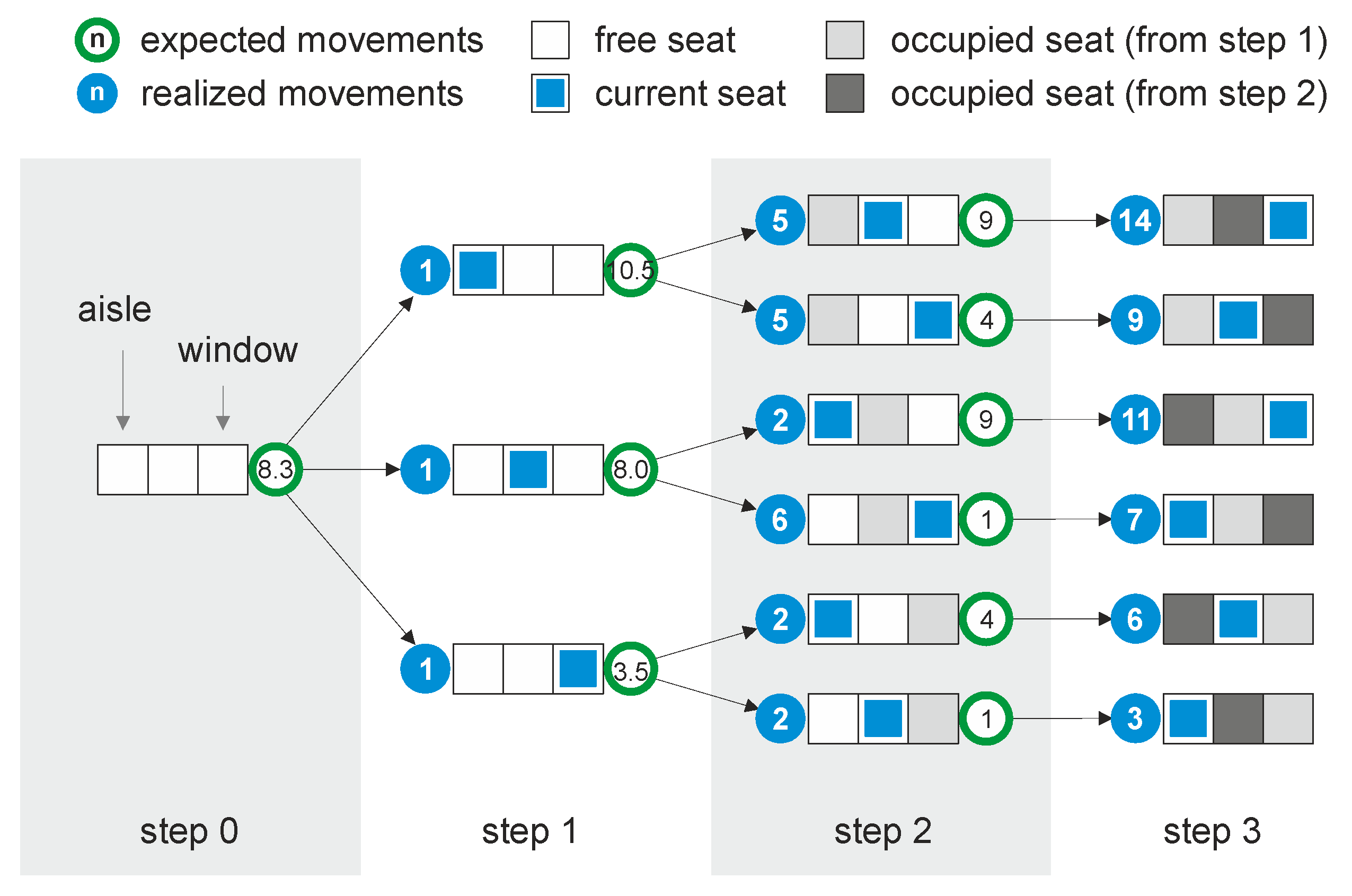
Figure 1 exhibits the transition between different seat row conditions and the corresponding development of the interference potential Pr (green circles). Here, Pr develops over time and decreases continuously if the seat row is filled up window seat first, followed by middle and aisle seat (Pr, step 0 = 8.3, Pr, step 1 = 3.5, Pr, step 2 = 1). This development results in only three passenger movements, since each passenger can directly step into the row without any interactions. If the boarding sequence starts with the aisle seat and ends with the middle seat, nine passenger movements are necessary, and Pr develops Pr, step 0 = 10.5, Pr, step 1 = 9.0, and Pr, step 2 = 9.
If other passengers are hindered in reaching their corresponding seat row and queue in the aisle, the negative effect of high Pr values increases and results in both additional waiting times and longer boarding time. This effect depends on the number of passengers who have to pass this row or wait in the queue to reach the seats located in front of this row. In a first approximation, only passing passengers with higher seat row numbers will be considered, by counting all seats which are currently free in the concerned row and the rows behind (number is stored as pb,r and modeled as exponential function with A as scaling factor). In (2), Pr is weighted by indirect interferences and summed up over all seat rows (m) to an aircraft-wide interference potential P. Furthermore, the difference between the minimum and maximum of P is considered as ΔP in the complexity metric as a measurement of convergence (Pr is the expected value in (2)).
The passenger arrival queue will also be taken into consideration (passengers who have already passed the boarding counter but have not been seated in the aircraft). Beginning with the first passenger i in the queue (with n members), each subsequently following passenger j is marked as negatively influenced (d = 1) if they want to reach a seat row with a higher seat row number than the passenger in front of him (3). An exponential function considers both weighted distance of passengers in the queue and expected seat row interference potential Pri for passenger i. While iterating over all passengers in the queue, the current passenger i will be virtually seated, which results in a continuous update of future seat row states for subsequently following passengers. Thus, a lower value of function k (3) indicates a lower level of influence between the passengers in the queue.
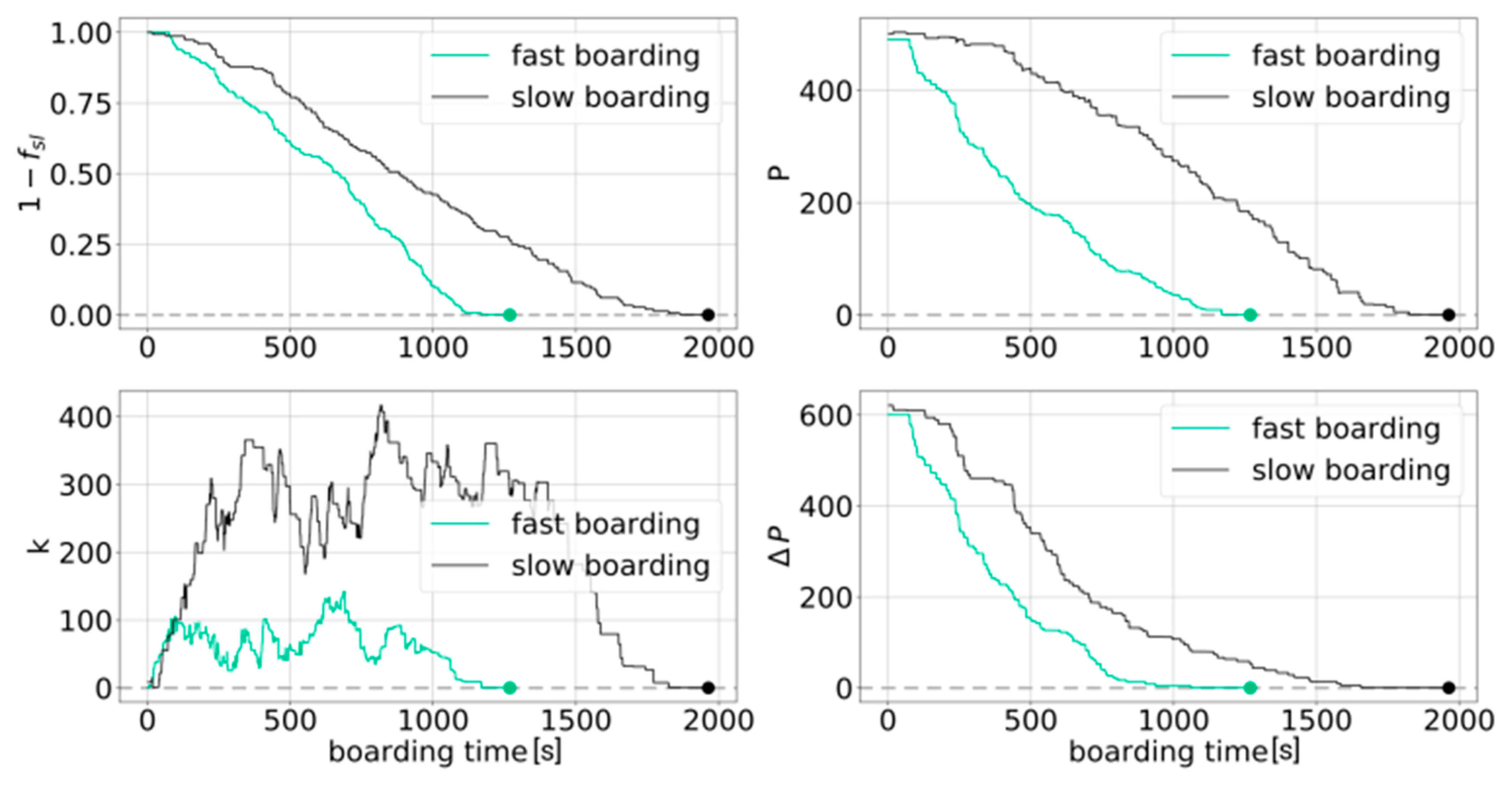
Finally, the complexity metric consists of four different indicators to evaluate the boarding progress. These indicators address the major, time-dependent drivers of boarding: Progress of seat load fsl (percentage of seated passengers), interference potential P (blocked seat rows), convergence of interference potential ΔP, and passenger sequence k (consider passengers boarded, but not seated). Figure 2 exhibits the complexity metric using a fast and slow boarding scenario. In the following, the seat load is defined as 1 − fsl to ensure a consistent behavior of all indicators, which end with a value of zero when the boarding is finished.
3. Machine Learning
To overcome resulting complexities and dynamic effects of passenger boarding, time predictions can be applied using advanced statistical procedures, such as neural networks. This section provides an overview concerning data transformation techniques to convert boarding time series to applicable datasets for machine learning (cf. Reference [55]), followed by a brief description of neural network structures and introduction of Long Short-Term Memory (LSTM) model.
3.1. Data Transformation
Similar to the majority of machine learning approaches, neural networks use supervised learning methods, and compare the predicted output against a reference value. For a given set of input variables {x(t)} and output variables {y(t)} an algorithm learns a functional dependency between input and output. The goal is to efficiently approximate the real (unknown) functional correlation and to predict output variables y ∈ {y(t)} by just having input variables x ∈ {x(t)}. In the context of passenger boarding, a sequence of observations is given as a dataset of time series demonstrating the boarding progress. Time series are differentiated into univariate (single variable) and multivariate (datasets) series. In the context of this paper, the multivariate time series consists of a complexity metric that consists of P and 1 − fsl. The boarding simulation provides time values for every single indicator of the metric, which could be used as multi-layer input considering current and past values. Since classical statistical methods do not perform well for this given problem, the application of complex and intelligent machine learning approaches is favored. As an example, the boarding dataset could be transformed to a supervised learning problem using P and 1 − fsl with a window size of one, as a multi-to-one time series (three input features and one output value, see Table 1, cf. Graves et al. [56]).
In order to follow up a multi-step prediction, the prediction datasets of the network are adjusted online (during active phase of application). Thus, we ensure that long-term predictions are made over different steps of time and train the network so that it is able to handle time-carried calculation errors.
3.2. Neural Network Models
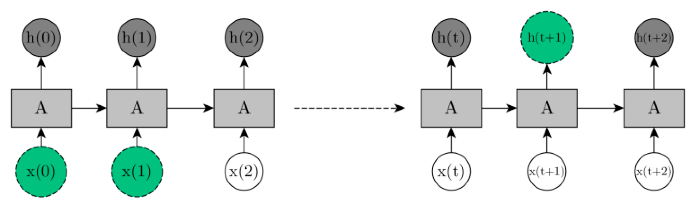
A standard recurrent neural network (RNN) computes the hidden vector sequence h = (h(1), …, h(T)) and output vector sequence y = (y(1), …, y(T)) for a given input sequence x = (x(1), …, x(T)) as shown in (4) and (5). The looped structure of RNN allows information to be passed from one step to the next. The term W denotes a weight matrix to the corresponding connections (e.g., Why is the hidden-output weight matrix), which basically comprise the parametrization sensibilities of the network. The b terms denote bias vectors as an extraction of the threshold function (e.g., by as the output hidden vector) and H is the hidden layer function. Usually H is an element-wise application of the logistic sigmoid function.
h(t) = H(Whyx(t) + Whhh(t − 1) + bh)
y(t) = Whyh(t) + by
Unlike classical feedforward neural networks, RNN models perform well in detecting and processing long-term correlations of inputs and outputs. Figure 3 depicts the effect of input vectors x(0) and x(1) to the hidden output h(t + 1). Such interdependencies, delayed over certain time steps, are essential part of a multivariate data analysis, as the dynamic of the system needs to be described through the influence of indicators to each other. LSTM networks address the problem of vanishing gradients of RNN by splitting in four inner gates and building so-called memory cells to store information in a long-range context. They also have a chain-like structure, but the module A (see Figure 3) has a different composition to explicitly address the long-term dependency problem.
Instead of having a single neural network layer, the inner workings of LSTM modules are divided into four gates. The LSTM structure is implemented through the following Equations (6)–(9). Here, σ and tanh represent the specific, element-wise applied activation functions of the LSTM, and i, f, o, c denote the inner-cell gates, namely the input gate, forget gate, output gate, and cell activation vectors respectively.
h i(t) = σ (Wxi x(t) + Whi h(t − 1) + Wci c(t − 1) + bi)
f(t) = σ (Wx f x(t) + Wh f h(t − 1) + Wc f c(t − 1) + bf)
c(t) = f(t) × c(t − 1) + i(t) × tanh(Wxc x(t) + Whc h(t − 1) + bc
o(t) = σ (Wxo x(t) + Who h(t − 1) + Wco c(t) + bo)
Gate c needs to be equal to the hidden vector h. As LSTM models are RNN based models, the overall composition is similar with regards to transforming an input set to an output set through a module A. In LSTM models A consists of a cell memory (information storage) with four gates: Computing input, updating cell, forget about certain information and setting output (cf. Reference [57]). To train RNN structures, a backpropagation through time algorithm is applied (cf. Reference [58]). It is used for calculating the gradients of the error with respect to weight matrices {W}. For a given batch size, which sets the amount of data after a gradient, an update is performed and the neuronal network can adjust its parametrization to retrieve given target values. With the capability to “store” knowledge, LSTMs overcome the RNN deficiency in handling vanishing gradients (a backpropagation of tanh values near 0 or 1 over time might lead to a blowing-up or disappearing). RNN-based models are characterized by the number of hidden layers (nhiddenlayer), the number of samples propagated through the network for each gradient update (batch-size), the number of trained epochs (nepoch) and the learning rate (η).
4. Simulation Framework and Application
The input data for the LSTM model is provided by the stochastic boarding model that covers several boarding strategies (cf. Reference [59]). We implemented the given RNN structures in Python 3.6 using the open-source deep learning library Keras 2.1.3 (frontend) with the open-source framework TensorFlow 1.5.0 (backend) and Scipy 1.0.0 (routines for numerical integration and optimization). Training and testing were performed on a GPU (NVIDIA Geforce 980 TI) with CUDA as the parallel computing platform and the application programming interface.
4.1. Simulation Framework
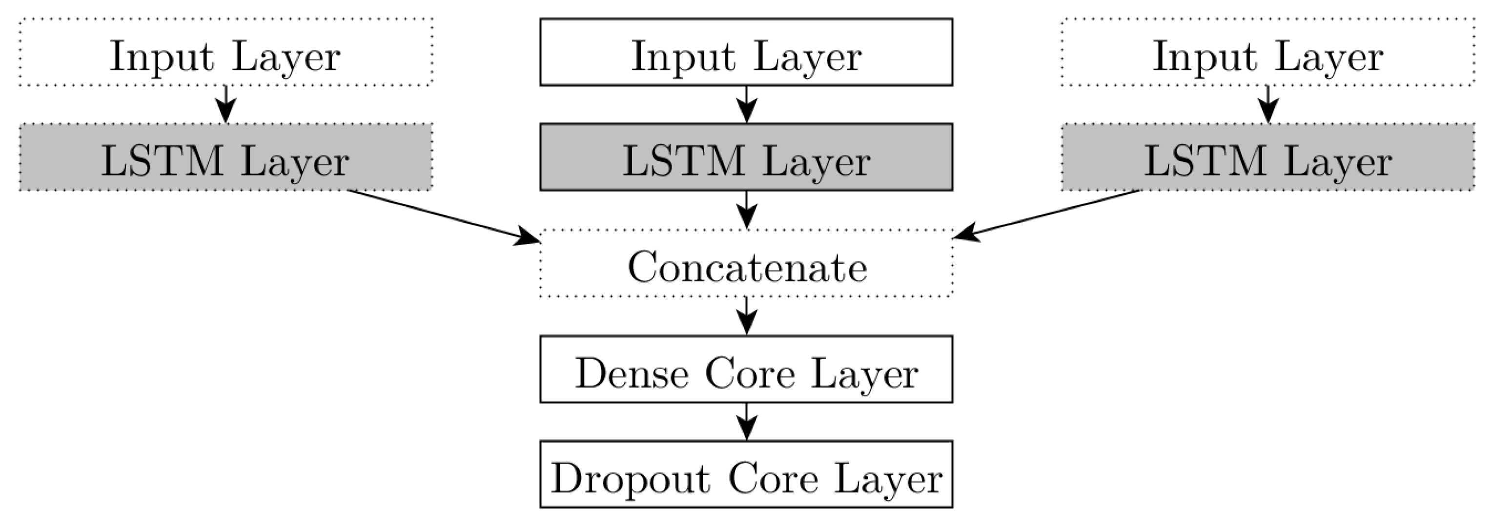
The simulation framework consists of fundamental components: Layers (LSTM, concatenate, input, dense, dropout), optimizers, and metric/loss functions. The structure of the implemented LSTM depends on the given scenario. For a one-dimensional application, one input layer is added to the model, followed by the LSTM recurrent layer, dense layer, and dropout layer. Figure 4 depicts the network structure for both cases: One-to-one (solid) and multi-to-multi regression (dotted). Each layer consists of specific tasks in the framework. The LSTM (recurrent) layer represents the specific machine learning model. The input layer is a Keras tensor object from the underlying backend (TensorFlow) and contains certain attributes to build a Keras model (knowing only in-/outputs).
The concatenate layer merges several inputs (list of tensors, with the same shape) and returns a single tensor. The dense layer is a regular densely-connected neural network layer and implements the fundamental output operation: Output = act(dot(input, kernel) + bias), where act is the element-wise activation function, kernel is a weights matrix created by the layer, and bias is a vector created by the layer. The dropout layer provides a regularization technique, which prevents complex co-adaptations on training data in neural networks (overfitting), by dropping a number of samples in the network (dropout rate). An optimizer is one of the two arguments required to finally compile the Keras model. Two optimizers are available: AdaGrad (adaptive gradient algorithm), modified stochastic gradient descent approach with per-parameter learning rate [60], and Adam (Adaptive Moment Estimation), a family of sub-gradient methods that dynamically incorporate knowledge of the geometry of the data observed in earlier iterations [61]. The optimizers are parametrized with the learning rates η = 0.01 and η = 0.001 for AdaGrad and Adam respectively. The loss function (optimization score function) of our model is the mean squared error (MSE).
4.2. Scenario Definition
In Table 2 an overview is given about the analyzed scenarios, focusing on the prediction of boarding progress of random and individual boarding strategies [59,62]. In scenario A, the prediction of random boarding is based on the learning of random boarding scenarios. In scenario B, the progress of individual boarding is predicted on the basis of all available boarding data sets, which additionally consists of block, back-to-front, outside-in, and reverse pyramid boarding strategies [59]. As input values P, 1 − fsl, or both are used to predict the output 1 − fsl. Both scenarios are computed for a given set of start times: 300 s, 400 s, and 600 s after boarding starts. Supervised learning demands for a separation of datasets into training, test and (obligatory) validation data. In our scenario analysis, we have 25,000 separate boarding results for random and individual boarding, and 100,000 boarding results from other strategies. We use 1000 randomly chosen boarding events to train the LSTM and 100 randomly chosen non-compiled /non-trained boarding events to evaluate the prediction.
4.3. Results
We trained the model within 18 different variants: Two main scenarios, each with three different input sets split into three different starting points. Similar experiments demonstrate several clues concerning useful combinations of certain optimizers and network structures depending on the amount of input data [42]. As we have two one-dimensional input sets (P, 1 − fsl), a more complex structure is needed, so we set nhiddenlayer to 120 for these variants (number of hidden LSTM layer next to input and output layer). In the case of uni-variate prediction we set nhiddenlayer to 40. A higher number of nhiddenlayer increases the ability of the network to understand complex data structures, but also increases the complexity of learning. AdaGrad works quite well with a more complex network structure, as its learning rate η is 10 times lower than η of Adam, which improves gradient-based learning in multi-branched inlays.
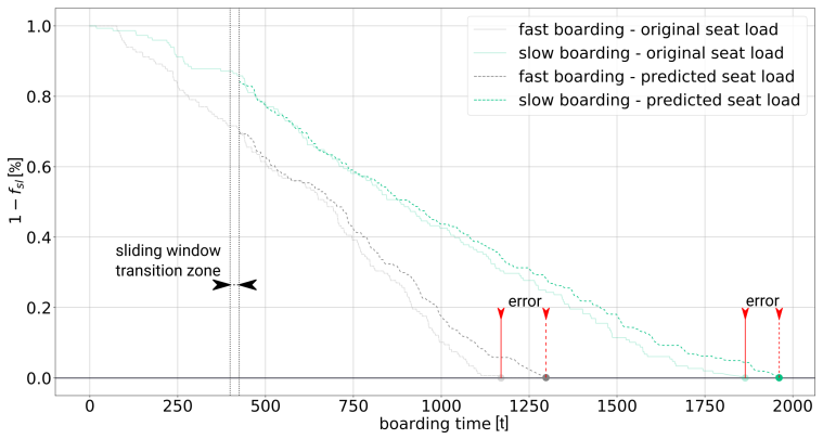
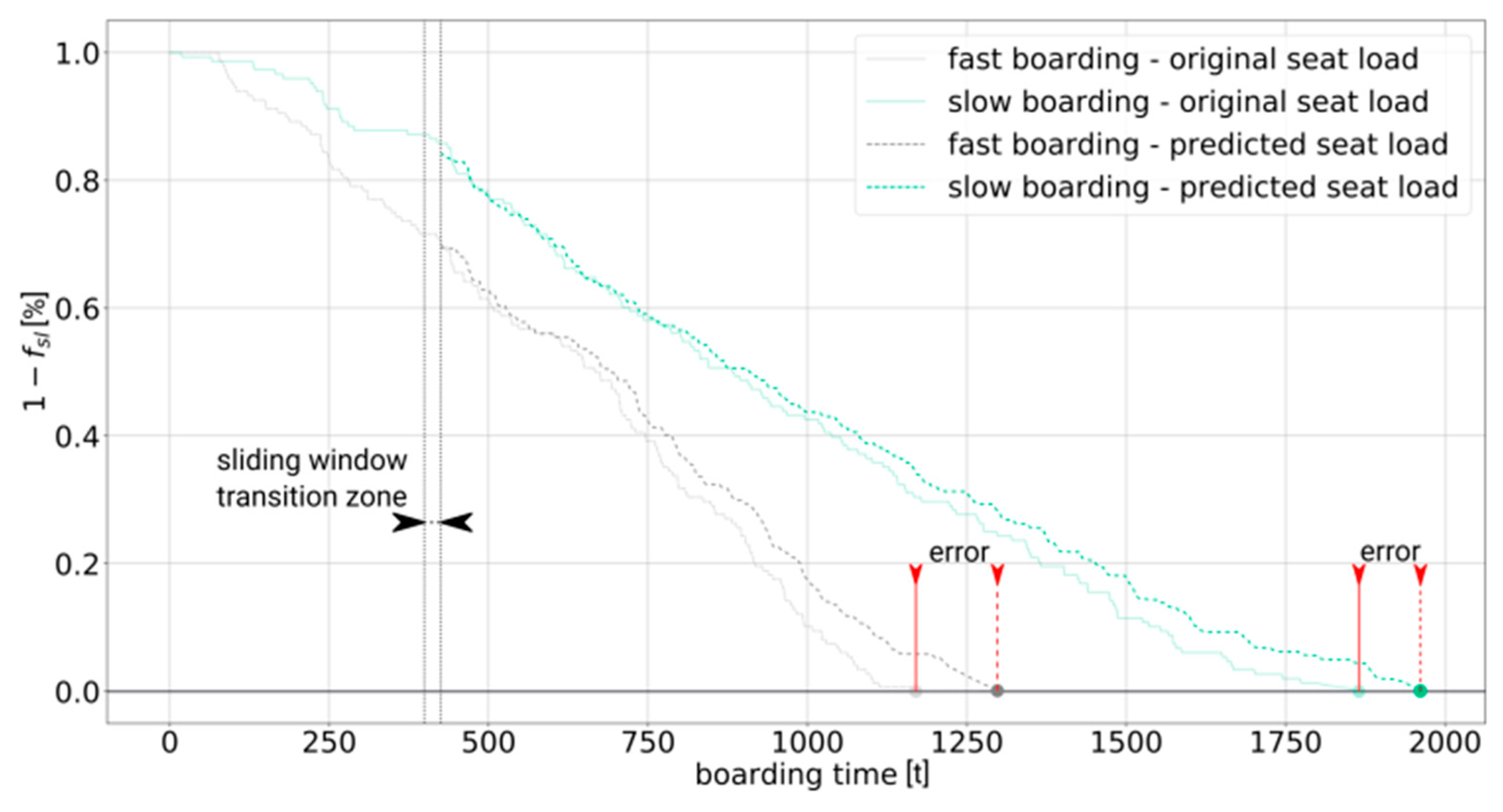
For both cases, uni- and multi-variate, we trained the model 20 times, which results in 20,000 training cycles. The window size is set to 25 and 5 for uni-variate and multi-variate respectively. The batch size (number of samples per gradient update) was set to 50 to balance computation time and accuracy. The model worked with a dropout rate of 0.5% for one-dimensional, 2.0% for multi-dimensional applications. Figure 5 exhibits results for slow and fast boarding progress. Here, the prediction starts at 400 s. The comparison of simulated (surrogate for real data) and predicted boarding progress demonstrates that the LSTM model is a promising candidate for boarding time prediction.
Table 3 provides an overview of the accuracy of each single model to the corresponding scenario including the computation time. The accuracy is measured as the mean error value of 100 tested scenarios after the training phase (1000 sample sets). In the table, cells are color coded, where red stands for MSE (learning error) >65%, green if MSE <25%, and yellow is in between these values. The major difference between scenario A and B is that in scenario A the LSTM is trained with corresponding data sets (random boarding input to predict random boarding). Scenario B uses all available boarding scenarios (random, block, back-to-front, outside-in, reverse pyramid, individual, cf. Reference [59]) for training to predict the progress of individually optimized boarding events. In doing so, the computational time t for training increases significantly (see Table 3). Due to the higher bandwidth of operational progresses in scenario B, the LSTM model is able to identify more interdependencies during the training process, which results in a more precise prediction.
As common statistical regression models would gradually suffer from calculation errors, neural network models receive the knowledge to end at a value of 0 (end of boarding) in every case of training. An insufficiently trained model might show bifurcations and chaotic behavior during the boarding process (red colored cells or NaN results), but would tend to reach the value 0 at the end. In our case, uni-variate inputs are not sufficient, and only multi-variate input results in reliable output values. Figure 6 shows the boarding progress (above) and time differences (below) for scenario A at specific progress steps using 400 s as start time for prediction. The box-plots of time differences refer to values illustrated in Table 3, using an interquartile ratio of 0.7. The red colored boxes include the last computed steps of the simulations (99% progress). The time variations at random boarding are significantly higher than that for the individual boarding, which results in higher inner progress differences as well. Both predictions show a positive and nearly symmetric offset over time.
5. Summary and Outlook
With this paper we provide the first approach to predicting the aircraft boarding progress, which is expected to significantly benefit aircraft turnaround operations in the future (e.g., precise scheduling by reduction of operational uncertainties). Since no operational data are available today from inside the aircraft cabin, we used a calibrated stochastic boarding model to provide reliable data for passenger movements. The data sets provide detailed status information about the current progress of aircraft boarding. This status contains seat load (percentage of seated passengers), interference potential (complexity measure considering already used seats), and the quality of the boarding sequence (chronological order of passenger arrival). These data are the input for a Long Short-Term Memory model, which is trained with time series data from the boarding simulation and enables a prediction of the final boarding time.
We show that the proposed complexity metric (multi-variate input) is a necessary element to predict the aircraft boarding progress, since uni-variate input results in non-converging behavior. Whilst the progress of the seat load was insufficient to reliably predict the boarding (high deviations), together with the complexity metric, the deviations are reduced by up to 75%. A closer look at differences between boarding progress and prediction shows an inherent positive offset. If this offset could be classified as constant, the prediction showed only a difference of ±20 s between prediction and underlying boarding simulation. Therefore, we see our LSTM approach as a promising candidate for extended investigations. In the next step, we want to extend our LSTM approach to improve the prediction process (e.g., robustness) and show the economic benefit for airport and airline operators.
Author Contributions
Conceptualization, M.S. and S.R.; Methodology, M.S. and S.R.; Software, M.S. and S.R.; Validation, M.S. and S.R.; Formal Analysis, M.S. and S.R.; Investigation, M.S. and S.R.; Resources, M.S.; Data Curation, M.S. and S.R.; Writing-Original Draft Preparation, M.S. and S.R.; Writing-Review & Editing, M.S.; Visualization, M.S. and S.R.; Supervision, M.S.; Project Administration, M.S.
Funding
This research received no external funding.
Conflicts of Interest
The authors declare no conflict of interest.
References
- Bronsvoort, J.; McDonald, G.; Porteous, R.; Gutt, E. Study of Aircraft Derived Temporal Prediction Accuracy using FANS. In Proceedings of the 13th Air Transport Research Society (ATRS) World Conference, Abu Dhabi, UAE, 27–30 June 2009. [Google Scholar]
- Mueller, E.R.; Chatterji, G.B. Analysis of Aircraft Arrival and Departure Delay. In Proceedings of the AIAA’s Aircraft Technology, Integration, and Operations (ATIO) 2002 Technical Forum, Los Angeles, CA, USA, 1–3 October 2002. [Google Scholar]
- EUROCONTROL Performance Review Commission. Performance Review Report—An Assessment of Air Traffic Management in Europe During the Calendar Year 2015; EUROCONTROL Performance Review Commission: Brussels, Belgium, 2015. [Google Scholar]
- Tielrooij, M.; Borst, C.; van Paassen, M.M.; Mulder, M. Predicting Arrival Time Uncertainty from Actual Flight Information. In Proceedings of the 11th USA/Europe Air Traffic Management R&D Seminar, Lisbon, Portugal, 23–26 June 2015. [Google Scholar]
- Rosenow, J.; Lindner, M.; Fricke, H. Impact of climate costs on airline network and trajectory optimization: A parametric study. CEAS Aeronaut. J. 2017, 8, 371–384. [Google Scholar] [CrossRef]
- Rosenow, J.; Fricke, H.; Schultz, M. Air traffic simulation with 4d multi-criteria optimized trajectories. In Proceedings of the Winter Simulation Conference (WSC), Las Vegas, NV, USA, 3–6 December 2017; pp. 2589–2600. [Google Scholar]
- Niklaß, M.; Lührs, B.; Grewe, V.; Dahlmann, K.; Luchkova, T.; Linke, F.; Gollnick, V. Potential to reduce the climate impact of aviation by climate restricted airspaces. Transp. Policy 2017. [Google Scholar] [CrossRef]
- Rosenow, J.; Fricke, H.; Luchkova, T.; Schultz, M. Minimizing contrail formation by rerouting around dynamic ice-supersaturated regions. AAOAJ 2018, 2, 105–111. [Google Scholar]
- Rosenow, J.; Förster, S.; Fricke, H. Continuous climb operations with minimum fuel burn. In Proceedings of the 6th SESAR Innovation Days, Delft, The Netherlands, 8–10 November 2016. [Google Scholar]
- Kaiser, M.; Schultz, M.; Fricke, H. Automated 4D descent path optimization using the enhanced trajectory prediction model. In Proceedings of the International Conference on Research in Air Transportation (ICRAT), Berkeley, CA, USA, 22–25 May 2012. [Google Scholar]
- Kaiser, M.; Rosenow, J.; Fricke, H.; Schultz, M. Tradeoff between optimum altitude and contrail layer to ensure maximum ecological en-route performance using the Enhanced Trajectory Prediction Model. In Proceedings of the 2nd International Conference on Application and Theory of Automation in Command and Control Systems, London, UK, 29–31 May 2012. [Google Scholar]
- Cook, A.J.; Tanner, G. European Airline Delay Cost Reference Values; Technical Report; EUROCONTROL Performance Review Unit: Brussels, Belgium, 2015. [Google Scholar]
- Airbus. Airbus A320 Aircraft Characteristics—Airport and Maintenance Planning; Airbus: Toulouse, France, 2017. [Google Scholar]
- Fricke, H.; Schultz, M. Improving Aircraft Turn Around Reliability. In Proceedings of the 3rd ICRAT, Fairfax, VA, USA, 1–4 June 2008; pp. 335–343. [Google Scholar]
- Fricke, H.; Schultz, M. Delay Impacts onto Turnaround Performance. In Proceedings of the 8th USA/Europe ATM Seminar, Napa, CA, USA, 29 June–2 July 2009. [Google Scholar]
- Schmidt, M. A Review of Aircraft Turnaround Operations and Simulations. Prog. Aerosp. Sci. 2017, 92, 25–38. [Google Scholar] [CrossRef]
- Jaehn, F.; Neumann, S. Airplane Boarding. Eur. J. Oper. Res. 2015, 244, 339–359. [Google Scholar] [CrossRef]
- Nyquist, D.C.; McFadden, K.L. A study of the airline boarding problem. J. Air Transp. Manag. 2008, 14, 197–204. [Google Scholar] [CrossRef]
- Mirza, M. Economic impact of airplane turn-times. AERO Q. 2008, 4, 14–19. [Google Scholar]
- Montlaur, A.; Delgado, L. Flight and passenger delay assignment optimization strategies. J. Trans. Res. Part C Emerg. Technol. 2017, 81, 99–117. [Google Scholar] [CrossRef]
- Oreschko, B.; Schultz, M.; Fricke, H. Skill Analysis of Ground Handling Staff and Delay Impacts for Turnaround Modeling. In Proceedings of the 2nd International Air Transport and Operations Symposium, Delft, The Netherlands, 28–29 March 2011; pp. 310–318. [Google Scholar]
- Oreschko, B.; Kunze, T.; Schultz, M.; Fricke, H.; Kumar, V.; Sherry, L. Turnaround prediction with stochastic process times and airport specific delay pattern. In Proceedings of the International Conference on Research in Airport Transportation (ICRAT), Berkeley, CA, USA, 22–25 May 2012. [Google Scholar]
- Ivanov, N.; Netjasov, F.; Jovanovic, R.; Starita, S.; Strauss, A. Air Traffic Flow Management slot allocation to minimize propagated delay and improve airport slot adherence. J. Transp. Res. Part A 2017, 95, 183–197. [Google Scholar] [CrossRef]
- Du, J.Y.; Brunner, J.O.; Kolisch, R. Planning towing processes at airports more efficiently. J. Trans. Res. Part E 2014, 70, 293–304. [Google Scholar] [CrossRef]
- Schultz, M.; Kunze, T.; Oreschko, B.; Fricke, H. Microscopic Process Modelling for Efficient Aircraft Turnaround Management; International Air Transport and Operations Symposium: Delft, The Netherlands, 2013. [Google Scholar]
- Kafle, N.; Zou, B. Modeling flight delay propagation: A new analytical-econometric approach. J. Transp. Res. Part B 2016, 93, 520–542. [Google Scholar] [CrossRef]
- Grunewald, E. Incentive-based slot allocation for airports. Transp. Res. Procedia 2016, 14, 3761–3770. [Google Scholar] [CrossRef]
- Schmidt, M.; Paul, A.; Cole, M.; Ploetner, K.O. Challenges for ground operations arising from aircraft concepts using alternative energy. J. Air Transp. Manag. 2016, 56, 107–117. [Google Scholar] [CrossRef]
- Milne, R.J.; Kelly, A.R. A New Method for Boarding Passengers onto an Airplane. J. Air Transp. Manag. 2014, 34, 93–100. [Google Scholar] [CrossRef]
- Qiang, S.-J.; Jia, B.; Xie, D.-F.; Gao, Z.-Y. Reducing Airplane Boarding Time by Accounting for Passengers’ Individual Properties: A Simulation Based on Cellular Automaton. J. Air Transp. Manag. 2014, 40, 42–47. [Google Scholar] [CrossRef]
- Milne, R.J.; Salari, M. Optimization of Assigning Passengers to Seats on Airplanes Based on Their Carry-on Luggage. J. Air Transp. Manag. 2016, 54, 104–110. [Google Scholar] [CrossRef]
- Zeineddine, H. A Dynamically Optimized Aircraft Boarding Strategy. J. Air Transp. Manag. 2017, 58, 144–151. [Google Scholar] [CrossRef]
- Fuchte, J. Enhancement of Aircraft Cabin Design Guidelines with Special Consideration of Aircraft Turnaround and Short Range Operations. Ph.D. Thesis, TU Hamburg-Harburg, Hamburg, Germany, 2014. [Google Scholar]
- Schmidt, M.; Nguyen, P.; Hornung, M. Novel Aircraft Ground Operation Concepts Based on Clustering of Interfaces; SAE Technical Paper 2015-01-2401; SAE: Warrendale, PA, USA, 2015. [Google Scholar]
- Schmidt, M.; Heinemann, P.; Hornung, M. Boarding and Turnaround Process Assessment of Single- and Twin-Aisle Aircraft. In Proceedings of the 55th AIAA Aerospace Sciences Meeting, Grapevine, TX, USA, 9–13 January 2017. AIAA 2017-1856. [Google Scholar]
- Schultz, M. Dynamic Change of Aircraft Seat Condition for Fast Boarding. J. Trans. Res. Part C Emerg. Technol. 2017, 85, 131–147. [Google Scholar] [CrossRef]
- Gwynne, S.M.V.; Yapa, U.S.; Codrington, L.; Thomas, J.R.; Jennings, S.; Thompson, A.J.L.; Grewal, A. Small-scale trials on passenger microbehaviours during aircraft boarding and deplaning procedures. J. Air Transp. Manag. 2018, 67, 115–133. [Google Scholar] [CrossRef]
- Schultz, M. Field Trial Measurements to Validate a Stochastic Aircraft Boarding Model. Aerospace 2017, 5, 27. [Google Scholar] [CrossRef]
- Li, Q.; Mehta, A.; Wise, A. Novel approaches to airplane boarding. UMAP J. 2007, 28, 353–370. [Google Scholar]
- Wang, K.; Ma, L. Reducing boarding time: Synthesis of improved genetic algorithms. In Proceedings of the 2009 Fifth International Conference on Natural Computation, Tianjin, China, 14–16 August 2009; pp. 359–362. [Google Scholar]
- Soolaki, M.; Mahdavi, I.; Mahdavi-Amiri, N.; Hassanzadeh, R.; Aghajani, A. A new linear programming approach and genetic algorithm for solving airline boarding problem. Appl. Math. Model. 2012, 36, 4060–4072. [Google Scholar] [CrossRef]
- Reitmann, S.; Nachtigall, K. Applying Bidirectional Long Short-Term Memories to Performance Data in Air Traffic Management for System Identification; Lecture Notes in Computer Science; Springer: Cham, Switzerland, 2017; Volume 10614, pp. 528–536. [Google Scholar]
- Maa, X.; Tao, Z.; Wang, Y.; Yu, H.; Wang, Y. Long short-term memory neural network for traffic speed prediction using remote microwave sensor data. Transp. Res. Part C 2015, 54, 187–197. [Google Scholar] [CrossRef]
- Lv, Y.; Duan, Y.; Kang, W.; Li, Z.; Wang, F.Y. Traffic flow prediction with big data: A deep learning approach. IEEE Trans. Intell. Transp. Syst. 2015, 16, 865–873. [Google Scholar] [CrossRef]
- Polson, N.G.; Sokolov, V.O. Deep learning for short-term traffic flow prediction. J. Trans. Res. Part C Emerg. Technol. 2017, 79, 1–17. [Google Scholar] [CrossRef] [Green Version]
- Zhou, M.; Qu, X.; Li, X. A recurrent neural network based microscopic car following model to predict traffic oscillation. J. Trans. Res. Part C 2017, 84, 245–264. [Google Scholar] [CrossRef]
- Zhong, R.X.; Luo, J.C.; Cai, H.X.; Sumalee, A.; Yuan, F.F.; Chow, A.H.F. Forecasting journey time distribution with consideration to abnormal traffic conditions. Transp. Res. Part C 2017, 85, 292–311. [Google Scholar] [CrossRef]
- Schultz, M.; Schulz, C.; Fricke, H. Efficiency of Aircraft Boarding Procedures. In Proceedings of the 3rd ICRAT, Fairfax, VA, USA, 1–4 June 2008; pp. 371–377. [Google Scholar]
- Schultz, M.; Kunze, T.; Fricke, H. Boarding on the Critical Path of the Turnaround. In Proceedings of the 10th ATM Seminar, Chicago, IL, USA, 10–13 June 2013. [Google Scholar]
- Schultz, M. A metric for the real-time evaluation of the aircraft boarding progress. J. Trans. Res. Part C Emerg. Technol. 2018, 86, 467–487. [Google Scholar] [CrossRef]
- Hochreiter, S.; Schmidhuber, J. Long Short-Term Memory. Neural Comput. 1997, 9, 1735–1780. [Google Scholar] [CrossRef] [PubMed]
- Schultz, M. Stochastic Transition Model for Pedestrian Dynamics. In Pedestrian and Evacuation Dynamics 2012; Springer: Cham, Switzerland, 2014; pp. 971–986. [Google Scholar]
- Schultz, M. Entwicklung Eines Individuenbasierten Modells zur Abbildung des Bewegungsverhaltens von Passagieren im Flughafenterminal. Ph.D. Thesis, TU Dresden, Saxony, Germany, 2010. Available online: http://nbn-resolving.de/urn:nbn:de:bsz:14-qucosa-85592 (accessed on 26 September 2018).
- Bazargan, M. A Linear Programming Approach for Aircraft Boarding Strategy. Eur. J. Oper. Res. 2007, 183, 394–411. [Google Scholar] [CrossRef]
- Yu, L.; Wang, S.; Lai, K.K. An integrated data preparation scheme for neural network data analysis. IEEE Trans. Knowl. Data Eng. 2006, 18, 217–230. [Google Scholar]
- Graves, A.; Fernandez, S.; Schmidhuber, J. Multi-Dimensional Recurrent Neural Networks. In Proceedings of the International Conference on Artificial Neural Networks (ICANN-2007), Porto, Portugal, 9–13 September 2007; Volume 4668, pp. 865–873. [Google Scholar]
- Gers, F.A.; Schmidhuber, J.; Cummins, F. Learning to Forget: Continual Prediction with LSTM. Neural Comput. 2000, 12, 2451–2471. [Google Scholar] [CrossRef] [PubMed]
- Hochreiter, S.; Bengio, Y.; Frasconi, P.; Schmidhuber, J. Gradient Flow in Recurrent Nets: The Difficulty of Learning Long-Term Dependencies; IEEE Press: Piscataway, NJ, USA, 2001. [Google Scholar]
- Schultz, M. Implementation and Application of a Stochastic Aircraft Boarding Model. J. Trans. Res. Part C Emerg. Technol. 2018, 90, 334–349. [Google Scholar] [CrossRef]
- Duchi, J.; Hazan, E.; Singer, Y. Adaptive subgradient methods for online learning and stochastic optimization. J. Mach. Learn. Res. JMLR 2011, 12, 2121–2159. [Google Scholar]
- Kingma, D.P.; Ba, J. Adam: A method for stochastic optimization. In Proceedings of the 3rd ICLR, Banff, AB, Canada, 14–16 April 2014. [Google Scholar]
- Steffen, J.H. Optimal Boarding Method for Airline Passengers. J. Air Transp. Manag. 2008, 14, 146–150. [Google Scholar] [CrossRef]
Figure 1.
Seat row progress (aisle seat right, window seat left) indicating movements/interactions expected (green circle) and realized (blue circle).
Figure 1.
Seat row progress (aisle seat right, window seat left) indicating movements/interactions expected (green circle) and realized (blue circle).

Figure 2.
Complexity metric to evaluate the boarding process and progress: Seat load (top left), interference potential (top right), boarding sequence (bottom left), and convergence of interference potential (bottom right).
Figure 2.
Complexity metric to evaluate the boarding process and progress: Seat load (top left), interference potential (top right), boarding sequence (bottom left), and convergence of interference potential (bottom right).

Figure 3.
Long-term interdependencies in RNN models encompassing a connection of input vectors x(0) and x(1) to the hidden output vector h(t + 1).
Figure 3.
Long-term interdependencies in RNN models encompassing a connection of input vectors x(0) and x(1) to the hidden output vector h(t + 1).

Figure 4.
Layer design of simulation framework.

Figure 5.
Prediction of seat load progress with LSTM model for two exemplary boarding events (prediction is based on the progress reached after 400 s).
Figure 5.
Prediction of seat load progress with LSTM model for two exemplary boarding events (prediction is based on the progress reached after 400 s).

Figure 6.
Scenario A (random input—random prediction)—progress (above) and time (below).


Table 1.
Multi-to-one time series using P (interference potential) and 1 − fsl (seat load).
| Time | Input A | Input B | Input C | Output |
|---|---|---|---|---|
| t | XA | XB | XC | Y |
| 0 | - | - | P(0) | 1 − fsl (1) |
| 1 | P(0) | 1 − fsl (1) | P(1) | 1 − fsl (2) |
| 2 | P(1) | 1 − fsl (2) | P(2) | 1 − fsl (3) |
| 3 | P(2) | 1 − fsl (3) | P(3) | prediction |
Table 2.
Scenario definition.
| Scenario | Boarding Strategy Learned | Boarding Strategy Predicted | Input from Complexity Metric | Prediction Start Time t (s) |
|---|---|---|---|---|
| A | random | random | {P, 1 − fsl, [P, 1 − fsl]} | {300, 400, 500} |
| B | all (random, block, back-to-front, outside-in, reverse pyramid, individual) | individual |
Table 3.
Results of computations of scenario A and scenario B.
| Scenario | Input (Uni-Variate) | Input (Uni-Variate) | Input (Multi-Variate) |
|---|---|---|---|
| A | [1 − fsl] | [P] | [P, 1 − fsl] |
| 300 s | NaNt = 1h 28min | NaNt = 1h 43min | 289.8 s t = 3h 02min |
| 400 s | 536.1 s t = 0h 30min | NaNt = 1h 01min | 143.7 s t = 2h 38min |
| 500 s | 301.8 s t = 0h 32min | NaNt = 0h 49min | 122.3 s t = 2h 12min |
| B | [1 − fsl] | [P] | [P, 1 − fsl] |
| 300 s | 603.1 s t = 1h 13min | NaNt = 1h 19min | 168,1 s t = 7h 38min |
| 400 s | 292.1 s t = 1h 12min | 389.9 s t = 1h 10min | 77.3 s t = 8h 01min |
| 500 s | 246.0 s t = 1h 08min | 412.4 s t = 1h 11min | 73.3 s t = 7h 54min |
NaN = not a number, prediction fails.
© 2018 by the authors. Licensee MDPI, Basel, Switzerland. This article is an open access article distributed under the terms and conditions of the Creative Commons Attribution (CC BY) license (http://creativecommons.org/licenses/by/4.0/).
Share and Cite
MDPI and ACS Style
Schultz, M.; Reitmann, S. Consideration of Passenger Interactions for the Prediction of Aircraft Boarding Time. Aerospace 2018, 5, 101. https://doi.org/10.3390/aerospace5040101
AMA Style
Schultz M, Reitmann S. Consideration of Passenger Interactions for the Prediction of Aircraft Boarding Time. Aerospace. 2018; 5(4):101. https://doi.org/10.3390/aerospace5040101
Chicago/Turabian StyleSchultz, Michael, and Stefan Reitmann. 2018. "Consideration of Passenger Interactions for the Prediction of Aircraft Boarding Time" Aerospace 5, no. 4: 101. https://doi.org/10.3390/aerospace5040101
Note that from the first issue of 2016, this journal uses article numbers instead of page numbers. See further details here.