Aerodynamic Design of a Laval Nozzle for Real Gas Using Hodograph Method


1
Moscow Institute of Physics and Technology, 9 Institutskiy per., Dolgoprudny, Moscow Region 141701, Russia
2
MIREA—Russian Technological University, 78 Vernadsky Avenue, Moscow 119454, Russia
*
Author to whom correspondence should be addressed.
Aerospace 2018, 5(3), 96; https://doi.org/10.3390/aerospace5030096
Submission received: 31 July 2018
/
Revised: 31 August 2018
/
Accepted: 3 September 2018
/
Published: 10 September 2018
Abstract
:We propose an approach for the design of the subsonic part of plane and axisymmetric Laval nozzles for real gases. The proposed approach is based on the hodograph method and allows one to solve the inverse design problem directly. Real gas effects are taken into consideration using the chemical equilibrium model. We present nozzle contours computed with the proposed method for a stoichiometric methane-air mixture. Results confirm that real gas effects have a strong influence on the nozzle shape. The described method can be used in the design of nozzles for rocket engines and for high-enthalpy wind tunnels.
1. Introduction
Supersonic nozzles are used in jet engines and in high-enthalpy wind tunnels for acceleration of a hot gas mixture in order to generate uniform supersonic flow. In the case of a rocket engine, the overall efficiency of the engine largely depends on the quality of the flow produced by the nozzle. In the case of a wind tunnel, flow uniformity directly influences the accuracy of experimental measurements. That is why in both cases there is a need for an accurate and robust method for the design of the nozzle.
Typically, it is desired to obtain a uniform supersonic flow with prescribed velocity and pressure values at the output cross-section of the nozzle. Sometimes, additional requirements should be satisfied, such as the absence of flow separations and shocks, limitations on the length of the nozzle, etc. Therefore, the design of a nozzle naturally leads to an inverse problem: to find the unknown nozzle shape knowing the flow parameters in some regions. It is worth mentioning that since transonic flow is very subtle and is prone to instability, such an inverse problem should be solved with very high accuracy.
If there is no separation in the boundary layer on the nozzle wall, then viscous effects have a negligible effect and the inviscid compressible gas model (Euler equations) can be used. In the supersonic region, the governing equations are of the hyperbolic type, and consequently, the inverse problem for plane and axisymmetric nozzles can be solved relatively easily by means of characteristic-based methods [1,2]. The main difficulty is the solution of the inverse problem in the subsonic region where the governing equations are elliptic.
Apparently, the first approach for this problem was based on the solution of the Cauchy problem for an elliptic second-order equation for the stream function [3]. Initial data (velocity distribution) were set on the axis of symmetry (or plane of symmetry), and then, a marching method in the orthogonal direction was applied. Such a Cauchy problem for an elliptic equation is the well-known Hadamard’s example of an ill-posed problem. Thereby, in order to obtain a generalized solution, some regularizations were applied, which led to an unavoidable error in the solution. Besides, it has been noted that nozzles computed using this approach are very long.
Modern methods for the design of a Laval nozzle are mostly based on the solution of the direct problem, like the majority of methods for aerodynamic optimization. The direct problem is to find a flow in a nozzle with a given shape and given inflow conditions. In contrast with the inverse problem, the direct problem is well posed and in most cases can be solved numerically. Usually in such optimization methods, the nozzle shape is parameterized using any convenient form (splines, Bezier curves), and the problem is formulated as a functional minimization problem for some objective function, for instance the norm of the deviation of output flow parameters from the desired ones [1,4,5].
One of the main advantages of such methods is their versatility: one can use any appropriate optimization procedure equipped with any black-box solver for the direct problem. Nevertheless, in many cases, the direct problem should be solved many times (from hundreds to thousands), which leads to large computational effort. Apart from that, at intermediate steps of the optimization procedure, the solution of the direct problem may produce complicated flow structures containing, for instance, flow separations and instabilities. In such cases, numerical methods for the direct problem can still produce large errors. That is why there is a need for methods that directly solve the inverse problem.
In the present study, we extend the approach for aerodynamic optimization, described in [6], which is applicable to inviscid plane and axisymmetric potential compressible flows of a perfect gas with constant adiabatic index. This approach utilizes a transformation from the spatial () plane to the hodograph plane. After such a transformation, velocity components become independent variables, while space coordinates become unknowns. This technique was successfully applied to a variety of problems including the design of spike nozzle [2], a nozzle guide vane [7] and Laval nozzles for experimental facilities [6] in “TsNIIMash” (Central Research Institute of Machine Building). Experimental measurements in these supersonic wind tunnels show that deviations from required the Mach number at the outlet of nozzles do not exceed 1% and confirm the robustness of the method. The problem statement in the hodograph plane provides the monotonicity of the velocity magnitude along the nozzle wall. In accordance with boundary layer theory, this property guarantees the separation of the free wall [8,9], which in turn justifies the applicability of the inviscid model. Another advantage of this method is that it provides the opportunity to design nozzles with a plane sonic surface. This allows one to design subsonic and supersonic parts of the nozzle separately.
The jet in rocket nozzles consists of a hot multicomponent mixture, and the typical temperature in the subsonic part of a nozzle is about 3000–4000 K. The same is appliable for high-enthalpy wind tunnels. Under such conditions, the perfect gas model is not valid, and real gas properties should be taken into account. In this paper, the described approach is extended to real gases. The extension is based on the fact that assuming chemical equilibrium or frozen reactions of the multicomponent mixture has a two-parameter equation of state [10]. Using this property, we obtain the general form of the equation for the stream function in the hodograph plane. To demonstrate the applicability of the extended approach, we use the two-parameter equation of state arising from the chemical equilibrium of the stoichiometric methane-air mixture.
The outline of the paper is the following: In Section 2, the main assumptions and governing equations are briefly described. Section 3 is devoted to the formulation or the inverse design problem in the hodograph plane. Section 4 contains short description of the chemical equilibrium model. Computational results and discussion are presented in Section 5.
2. Potential 2D Flows of Real Gases
We consider plane or axisymmetric steady potential flow of an inviscid compressible gas obeying an arbitrary two-parameter equation of state. We will use the following notation throughout this paper:
- (), physical coordinates,
- , density,
- p, pressure,
- u, v, the x and y components of velocity,
- , velocity magnitude,
- , the angle between the velocity vector and x-axis
- , the Mach number, a being the speed of sound,
- e, internal energy,
- , enthalpy,
- , full enthalpy,
- S, entropy,
- , , stream function and potential, defined by , .
It was proven in [11] that flow potentiality implies that the entropy and stagnation enthalpy are constant, just like in the case of ideal gas with a constant adiabatic index:
Using these first integrals, the system of Euler equations can be reduced to the system of two equations:
The first equation is the continuity equation, and the second equation reflects the fact that the flow is irrotational.
Due to the existence of the first integrals, the density, Mach number and other parameters of potential flow are functions of the velocity magnitude only:
and are uniquely determined from the inlet conditions.
The hodograph transformation is a mapping from () or () to (). Properties of this transformation had been established in [6]. The change of variables can be performed easily with the help of expressions like:
Similarly, all derivatives in the equations can be expressed via derivatives with respect to and the Jacobian of hodograph mapping . This leads to the following equation:
Here:
Coordinates are connected with through the relations:
3. Inverse Problem Formulation in the Hodograph Plane
Since isolines of the function correspond to stream lines, we can formulate the inverse nozzle design problem as a well-posed boundary problem for second-order Equation (8) in the hodograph plane [6].
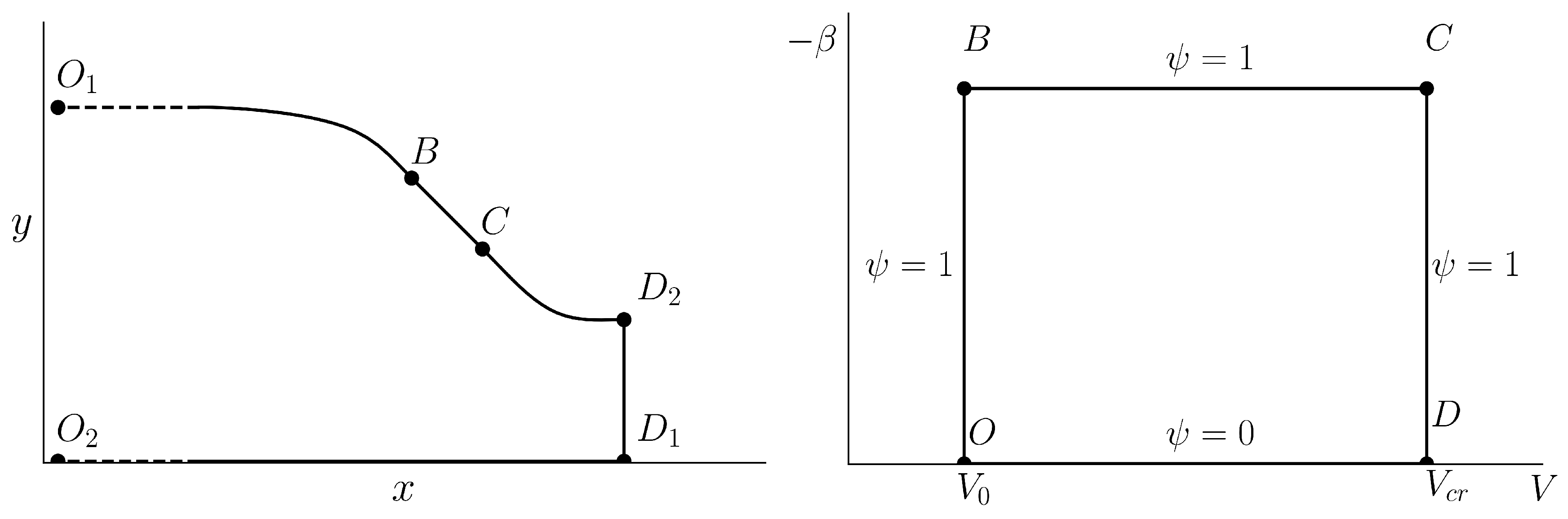
In this paper, we utilize one of many possible formulations of the inverse problem (which is depicted schematically in Figure 1 due to its simplicity. We consider an infinitely long nozzle; uniform flow with velocity , which is parallel to the x axis, comes from infinity and approaches sonic velocity on line .
As mentioned, such a scheme allows one to design subsonic and supersonic parts of the nozzle separately, which is very convenient.
We require that along the curvilinear part of the nozzle wall, the velocity magnitude is constant and equal to . Consequently, and are mapped to the point O in the hodograph plane, and is mapped to the vertical line segment.
Furthermore, we require that along the rectilinear part , the velocity magnitude is monotonically increased from to critical value such that . Since along , it is mapped to the horizontal line segment. Finally, we assume that along the part, the velocity magnitude equals , so it is mapped to the vertical line segment. Both ends of the straight sonic line are mapped to the point D.
As mentioned, the part corresponds to one stream line and the part to another, which leads to a straightforward statement of the boundary conditions.
The described flow scheme results in a very simple boundary problem for elliptic Equation (8) with degeneration on the boundary, which can be solved easily using, for instance, the five-point finite difference scheme on a uniform Cartesian grid. It should be noted that discontinuity in the boundary conditions does not complicate the numerical procedure, since corner points are not used in the difference scheme.
4. Chemical Equilibrium Model
At high temperatures, chemical reactions significantly change the chemical composition of the gas mixture and, consequently, all the thermodynamic properties. That is why reactions should be taken into account when designing a high-enthalpy nozzle.
In general case of chemical nonequilibrium additional equations for the concentrations of each component should be solved, which are coupled with the equations of motion:
Fixing p and T locally and linearizing the right-hand side at the equilibrium concentrations , for which , we come to the following system:
which has the solution:
From this expression, it is clear that the relaxation time, e.g., the characteristic time for a mixture to reach the equilibrium, is determined by the smallest in absolute value eigenvalue of the Jacobian matrix: . In the particular case of a simple reaction, this estimate is reduced to , where is the reaction rate constant. In the general case, depends both on the reaction rate constants of all individual backward and forward reactions and the concentrations of each component.
If this time is very small compared to characteristic time associated with gas motion, we can assume that at each point, the mixture is in local chemical equilibrium. Another extreme case of frozen reaction corresponds to large values of the ratio . The advantage of both models is that the mixture can be described by the two-parameter equation of state, which is easily incorporated in the framework of Section 2.
Here, we give a simple estimate for based on the relaxation times of individual reactions. To demonstrate the applicability of the described hodograph-based method, we consider a stoichiometric methane-air mixture with 16 components: O, N, C, H, , , , , , , , , , , , . Equilibrium concentrations for K and 4000 K and atmosphere are depicted in Figure 2. The relaxation times of dissociation-recombination reactions, which play the most important role in our case, lying below s for the considered temperature range [12]. There are a few slow reactions, for instance the nitrogen oxidation reaction. The relaxation time of this reaction varies from one second at K to about s at 4000 K [12]. However, the molar fractions of both and are very small at low temperatures, and the effect of such reactions on the thermodynamic properties of the mixture is negligible.
The characteristic time of macroscopic motion in the subsonic part of a nozzle , where L is the nozzle length and is the speed of sound at the sonic surface. For m, m/s, we obtain the estimate . Thus, in our case, , and the chemical equilibrium model can be considered. We should note that for more complex mixtures, one should use more careful estimates based on the detailed kinetic scheme and reaction rate constants.
The requirement is often not met in the supersonic part of the nozzle, if the density is small. Nevertheless, the standard approach is to use the equilibrium approximation in the subsonic part and the frozen flow approximation in the supersonic part of the nozzle [10]. Since the frozen flow is a two-parameter gas, the proposed hodograph-based method can be applied to the supersonic part as well.
The calculation of the equilibrium composition in a gas is performed by means of a numerical solution of the law of mass action. The chemical equilibrium conditions can be written in the form:
where is the molar concentration of the i-th component, the equilibrium constant of the i-th component and the stoichiometric coefficient.
With equations for the molar and mass concentration of components, the law of mass action can be formulated in the form of the material balance system of equations with respect to the molar concentrations of the components consisting of L linearly independent equations. When the system is solved, it is possible to determine N unknown molar concentrations . The system is solved by Newton’s method. In this case, the accuracy of the solution depends on the accuracy of the equilibrium constants, which can be expressed through the free Gibbs energy. For the Gibbs energy, we use approximations from [13,14]. The approximations have the following form:
where T is the temperature. Therefore, the equilibrium constants can be expressed through the Gibbs energy from the following equations:
where is the gas constant and the tabular values of the molar heat of the reaction. From the obtained molar concentrations of the components, the molecular weight of the mixture can be calculated. The density of the mixture is calculated from the equation of state of an ideal gas, taking into account the molecular weight of the mixture.
To calculate the molar enthalpy, the following formula is used:
where is the tabular values of the molar enthalpy of formation of the k-th component. The specific enthalpy of the mixture is found from the specific enthalpies of the components:
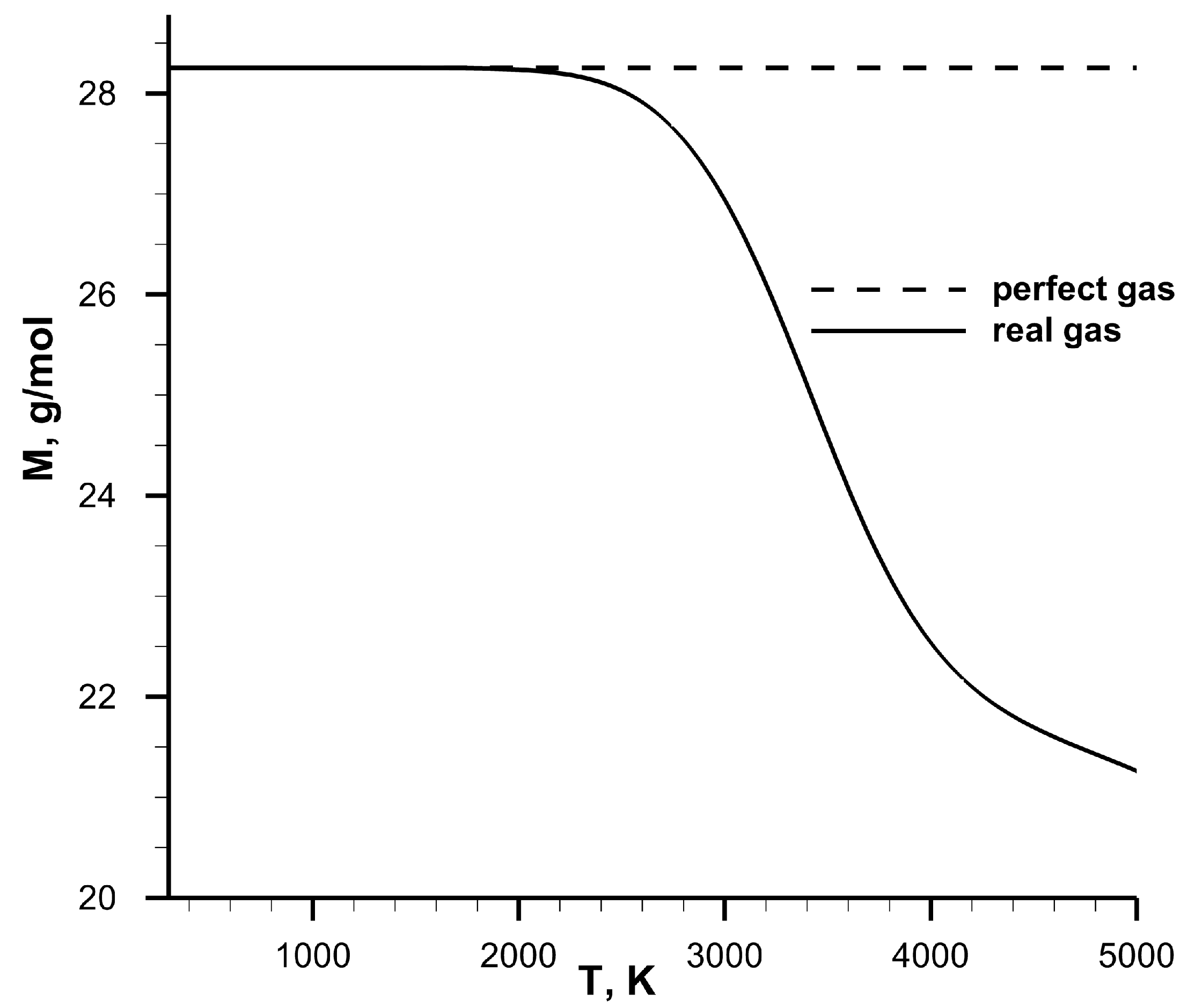
The dependence of molar mass on T for the equilibrium stoichiometric methane-air mixture at atm is shown in Figure 3. This dependence demonstrates that at high temperatures (>1800 K), real gas effects should be taken into account.
The described procedure yields all thermodynamic parameters of the chemically-equilibrated mixture as functions of p and T. However, the coefficients in Equation (8) depend on enthalpy and entropy. That is why an intermediate procedure is necessary to connect these two parameterizations.
Let us assume that we want to compute some quantity at . At first, we find the equations of entropy isolines in the plane:
Initial condition for this ODE, which follows from the inlet condition for the nozzle, defines one curve , corresponding to some implicit value of entropy . After that, solving the equation:
we obtain pair (). It should be noted that Equation (12) is integrated only once for the given problem, yet (13) is solved for each value of V in each mesh node.
5. Results and Discussion
The boundary problem for Equation (8) depicted in Figure 1 is solved using the standard second order five-point finite-difference scheme on a Cartesian mesh. In the axisymmetric case, the nonlinear right-hand side term in Equation (8) is updated iteratively.
The color map of the solution for K, atm, is illustrated in Figure 4. The x axis corresponds to velocity magnitude V and the y axis to velocity angle . Nozzle contours are computed from the solution by integrating Equation (10) along the right, upper and left boundaries (where ) with the second order explicit Runge–Kutta method. Serial computations show that 200 nodes along each direction are sufficient to obtain the mesh independent solution.
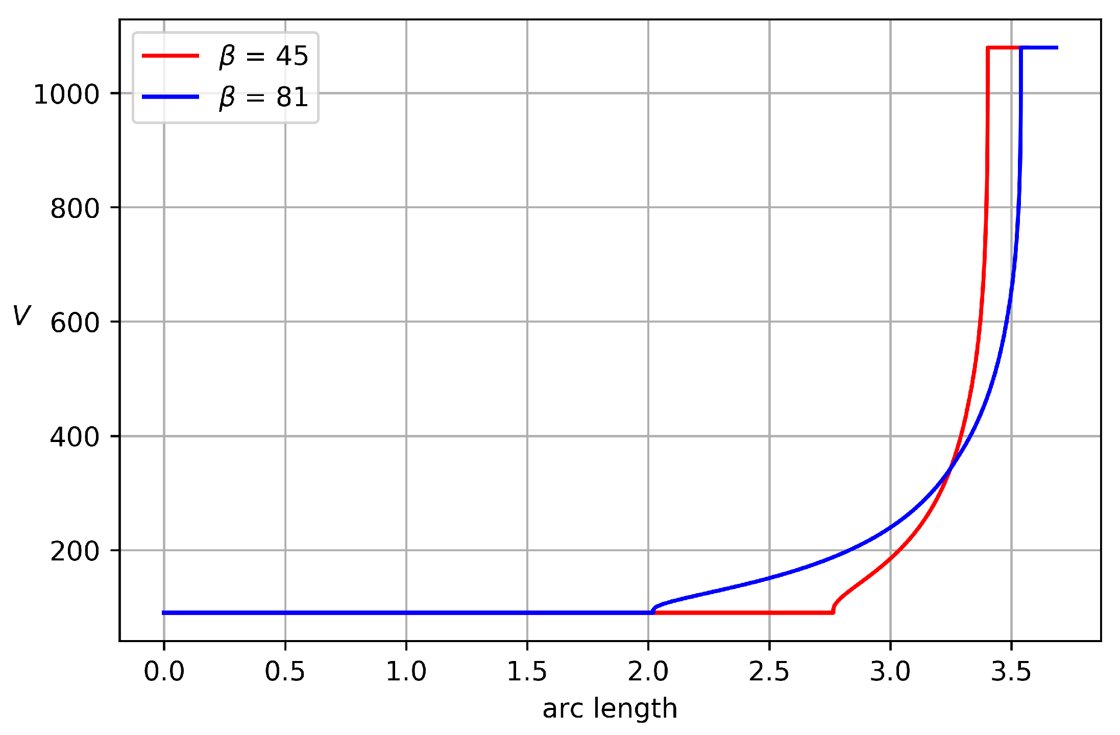
Computed contours for different values of inlet temperature and for atm are plotted in Figure 5. We present contours only for the plane case as it is more convenient for comparison.
As expected, the nozzle shape strongly depends on T since the chemical composition significantly changes along the nozzle. In the case of K, there are no reactions, and the computed contour coincides with that computed using the perfect gas model. It is worth noting that the proposed method allows one to compute contours with any including .
The presented contours demonstrate that the longest part of the contour is that on which the velocity magnitude is constant.
Two velocity profiles along the nozzle wall for , atm are depicted in Figure 6. As has been already mentioned, on of the advantages of the proposed method is that it provides monotone acceleration of the flow along the nozzle wall, which in turn guarantees the separation of the free flow. It can be seen from Figure 6 that acceleration can be very fast if the straight part of the nozzle contour is short. This drawback can be eliminated by using non-rectangular domains in the hodograph plane. In this case, we can provide a strictly increasing velocity profile.
6. Conclusions
In this paper, a novel approach for the design of the subsonic part of the axisymmetric and the plane Laval nozzle is presented. The approach is based on the hodograph method, developed earlier for the potential flow of perfect gases, and the chemical equilibrium model. The extension to real gases is straightforward since real gas properties, usually available in tabular form, are encapsulated in the coefficients of equations on the stream function.
The applicability of the proposed approach is demonstrated by the computation of plane nozzle contours for different values of inlet temperature and pressure.
In our future work, we will investigate the applicability of the proposed method using a comparison of the flow obtained from the inverse problem with the solution of the direct problem with computed contours. Such a comparison will allow us to estimate the influence of uncertainty in the input data on the flow in the nozzle. Furthermore, we will try to use polygonal domains in the hodograph plane in order to provide a strict increase of the velocity along the nozzle wall.
Author Contributions
A.C. developed numerical methods for inverse problem and wrote the draft; M.P. developed methods for chemical part; R.D. performed calculations and made comparisons; E.S. was responsible for conceptualization.
Funding
This work was supported by the Ministry of Education and Science of the Russian Federation, unique project identifier RFMEFI60417X0181 (State assignment no. N14.604.21.0181 dated by 26.09.2017).
Conflicts of Interest
The authors declare no conflicts of interest.
References
- Kraiko, A.; P’yankov, K. Effective direct methods for aerodynamic shape optimization. Comput. Math. Math. Phys. 2010, 50, 1546–1552. [Google Scholar] [CrossRef]
- Shifrin, E.; Kim, C. Shaping a nozzle with a central body by the chaplygin method. Dokl. Phys. 2005, 50, 143–146. [Google Scholar] [CrossRef]
- Pirumov, U.; Suvorova, V. Numerical solution of an inverse problem of nozzle theory for a two-phase gas-particle mixture. Fluid Dyn. 1986, 21, 595–603. [Google Scholar] [CrossRef]
- Heath, C.; Gray, J.; Park, M.; Nielsen, E.; Carlson, J.R. Aerodynamic shape optimization of a dual-stream supersonic plug nozzle. In Proceedings of the 53rd AIAA Aerospace Sciences Meeting, Kissimmee, FL, USA, 5–9 January 2015. [Google Scholar] [CrossRef]
- Allman, J.G.; Hoffman, J.D. Design of maximum thrust nozzle contours by direct optimization methods. AIAA J. 1981, 19, 750–751. [Google Scholar] [CrossRef]
- Shifrin, E.G.; Belotserkovskii, O.M. Transonic Vortical Gas Flows; Wiley: Hoboken, NJ, USA, 1996. [Google Scholar]
- Shifrin, E.; Kamenetskii, D. Hodograph method for turbine nozzle guide vane profiling. In Proceedings of the ECCOMAS Computational Fluid Dynamics Conference, Paris, France, 9–13 September 1996; pp. 623–628. [Google Scholar]
- Anderson, J.D., Jr. Fundamentals of Aerodynamics; Tata McGraw-Hill Education: New York, NY, USA, 2010. [Google Scholar]
- Oleinik, O.A. Mathematical problems of boundary layer theory. Russ. Math. Surv. 1968, 23, 1. [Google Scholar] [CrossRef]
- Lunev, V. Real Gas Flows with High Velocities; CRC Press: Boca Raton, FL, USA, 2009. [Google Scholar]
- Shifrin, E. Potential 2D flows of real gases. Invariant equations in natural coordinates. Hodograph transformation. Int. J. Appl. Eng. Res. 2015, 10, 34190–34193. [Google Scholar]
- Zel’Dovich, Y.B.; Raizer, Y.P. Physics of Shock Waves and High-Temperature Hydrodynamic Phenomena; Courier Corporation: North Chelmsford, MA, USA, 2012. [Google Scholar]
- Gurvich, L.V.; Veyts, I.V.; Medvedev, V.A.; Khachkuruzov, G.A.; Yungman, V.S.; Bergman, G.A.; Baybuz, V.F.; Iorish, V.S.; Yurkov, G.N.; Gorbov, S.I.; et al. Thermodynamic Properties of Individual Substances; Hemisphere Publishing Corp.: New York, NY, USA, 1989; Volume 1, Part 2; p. 340. [Google Scholar]
- D’angola, A.; Colonna, G.; Gorse, C.; Capitelli, M. Thermodynamic and transport properties in equilibrium air plasmas in a wide pressure and temperature range. Eur. Phys. J. D 2008, 46, 129–150. [Google Scholar] [CrossRef]
Figure 1.
Hodograph transformation for the flow in the nozzle.

Figure 2.
Molar fractions of the components for temperatures of 2000 K and 4000 K.
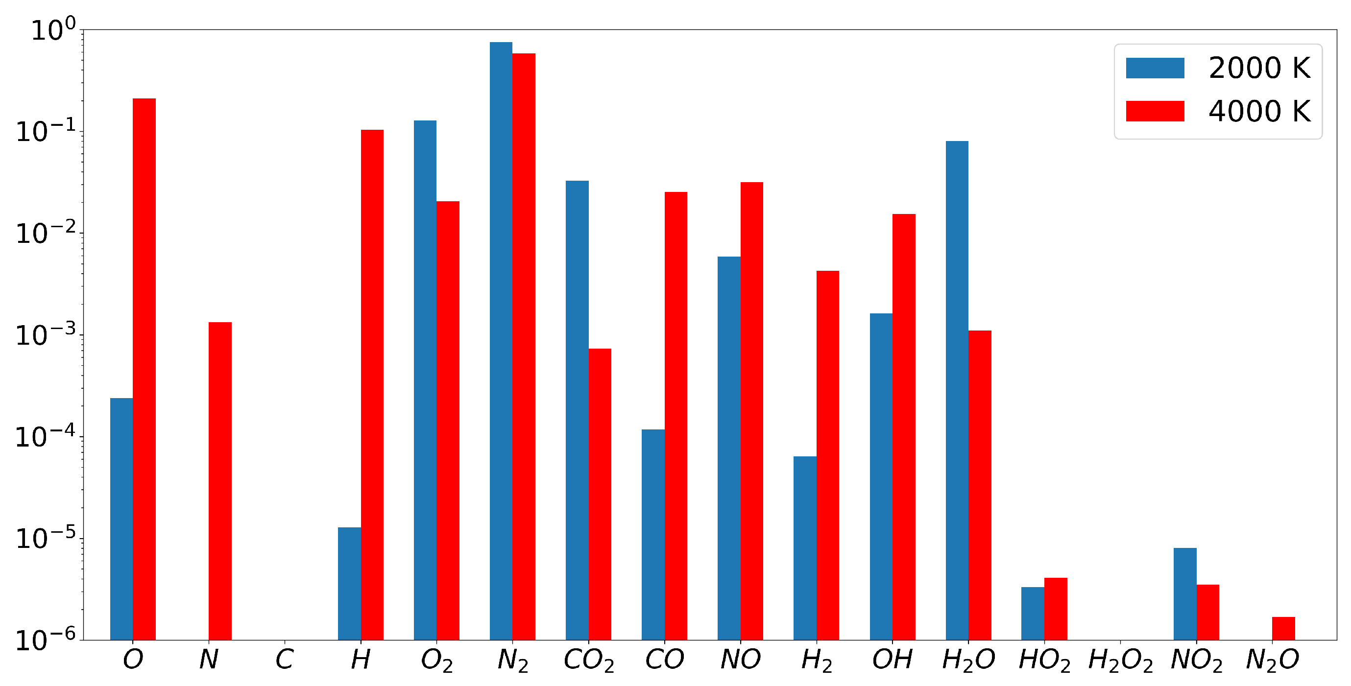
Figure 3.
Molar mass of the methane-air mixture.

Figure 4.
Color map of the solution of the boundary value problem in the hodograph plane.
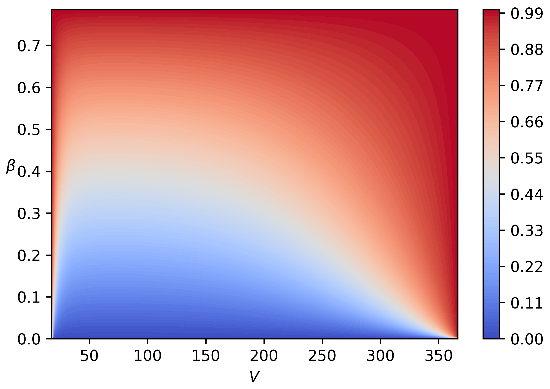
Figure 5.
Nozzle contours.
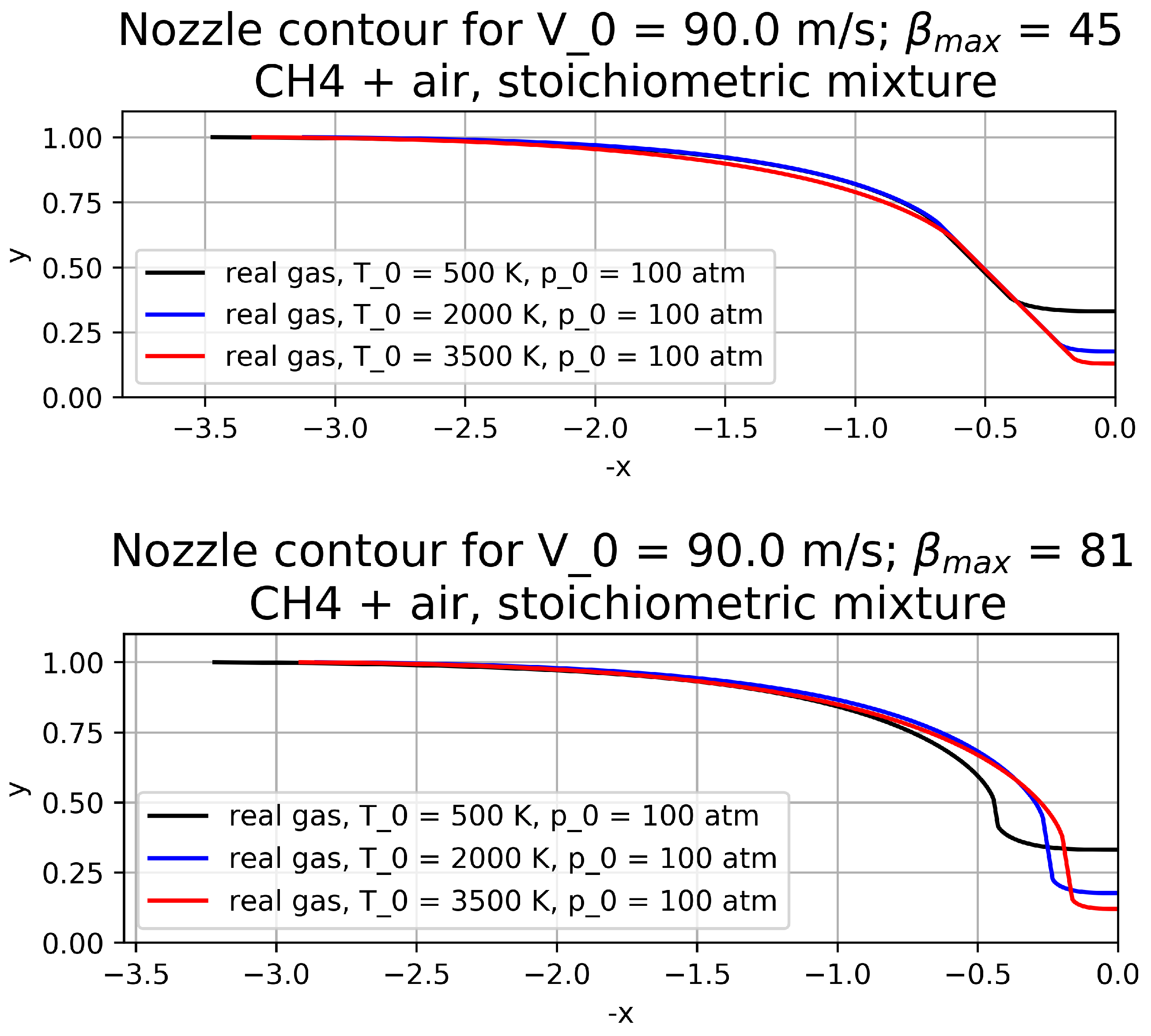
Figure 6.
Velocity magnitude along the nozzle wall.

© 2018 by the authors. Licensee MDPI, Basel, Switzerland. This article is an open access article distributed under the terms and conditions of the Creative Commons Attribution (CC BY) license (http://creativecommons.org/licenses/by/4.0/).
Share and Cite
MDPI and ACS Style
Chikitkin, A.; Petrov, M.; Dushkov, R.; Shifrin, E. Aerodynamic Design of a Laval Nozzle for Real Gas Using Hodograph Method. Aerospace 2018, 5, 96. https://doi.org/10.3390/aerospace5030096
AMA Style
Chikitkin A, Petrov M, Dushkov R, Shifrin E. Aerodynamic Design of a Laval Nozzle for Real Gas Using Hodograph Method. Aerospace. 2018; 5(3):96. https://doi.org/10.3390/aerospace5030096
Chicago/Turabian StyleChikitkin, Aleksandr, Mikhail Petrov, Roman Dushkov, and Ernest Shifrin. 2018. "Aerodynamic Design of a Laval Nozzle for Real Gas Using Hodograph Method" Aerospace 5, no. 3: 96. https://doi.org/10.3390/aerospace5030096
Note that from the first issue of 2016, this journal uses article numbers instead of page numbers. See further details here.