Nonlinear Model Predictive Control for Unmanned Aerial Vehicles ^†

Abstract

This paper discusses the derivation and implementation of a nonlinear model predictive control law for tracking reference trajectories and constrained control of a quadrotor platform. The approach uses the state-dependent coefficient form to capture the system nonlinearities into a pseudo-linear system matrix. The state-dependent coefficient form is derived following a rigorous analysis of aerial vehicle dynamics that systematically accounts for the peculiarities of such systems. The same state-dependent coefficient form is exploited for obtaining a nonlinear equivalent of the model predictive control. The nonlinear model predictive control law is derived by first transforming the continuous system into a sampled-data form and and then using a sequential quadratic programming solver while accounting for input, output and state constraints. The boundedness of the tracking errors using the sampled-data implementation is shown explicitly. The performance of the nonlinear controller is illustrated through representative simulations showing the tracking of several aggressive reference trajectories with and without disturbances.

1. Introduction

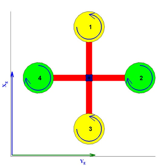
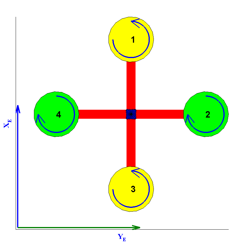
A quadrotor helicopter platform (often just called a quadrotor) is an under-actuated helicopter with two pairs of rotors in a cross-configuration capable of spinning at different angular velocities in order to achieve translational and rotational motion. Rotor pair $(1,3)$ spins in one direction, while the pair $(2,4)$ spins in the opposite (see Figure 1).

The different motions the quadrotor can perform are: (a) vertical motion: simultaneous change in rotor speed; (b) roll motion: imbalance in the rotor speed of pair $(2,4)$; (c) pitch motion: imbalance in the rotor speed of pair $(1,3)$; (d) yaw motion: imbalance between all rotors.

Quadrotors have gained popularity as research platforms because of their simplicity of design and low cost of manufacturing. Because they are challenging vehicles to control, wherever operated in an indoor environment or in the open field, they serve as great platforms for research. They also possess many advantages over standard helicopters in terms of safety and efficiency at small sizes [1]. There are many applications for a quadrotor platform, both in the military and the civil sectors, which are summarized quite extensively in [2,3,4,5,6].

To enable autonomous operations of a quadrotor, the research community typically focuses on the following aspects of the quadrotor: kinematics and dynamics of the vehicle; trajectory generation (path planning); guidance, navigation and control.

The focus of this paper is to synthesize a nonlinear model predictive control law for tracking a trajectory to be followed by a quadrotor. The applications are typically way-point navigation and tracking certain agile maneuvers [7,8,9,10]. Since the quadrotor can only generate forces normal to the plane that contains the rotors, the translational and rotational dynamics are significantly coupled. This restricts the quadrotor from performing certain maneuvers [11] that are possible with a fixed wing aircraft and the more conventional helicopter. In what follows, some key works relevant to these topics are summarized, and the layout of the paper is outlined.

A significant amount of research has been performed in the area of trajectory generation and constrained control of unmanned vehicles that apply to quadrotors alike. The work in [12,13] discusses the generation of trajectories for robots, wherein a spline interpolation method is used to solve a minimum time optimization problem, while staying under torque and velocity constraints. The work in [14] also used a spline interpolation method to generate optimal-time trajectories and applied it to a micro-quadrotor. For reference trajectory generation, [7] develops the governing equations of motion and describes the trajectories as algebraic functions of a flat output: outputs that can express the states and inputs of the system in terms of its outputs and their derivatives [15]. This approach facilitates the automatic trajectory generation for the system. In [9], trajectories are generated by designing a sequence of controllers to drive the system to a desired goal state. The works in [1,16] discuss the design of safe, aggressive maneuvers and control for a back flip trajectory. The work in [17] constructed a dynamically feasible, desired speed profile for a given sequence of waypoints. The authors in [18,19] worked on trajectory generation for quadrotors by implementing dynamic constraints to an optimal control method and verified the existence of optimal trajectories. The work in [20] addresses the problem of quadrotor trajectory generation and tracking while carrying a suspended payload. They solved this by developing an optimal controller based on the dynamic programming technique: breaking down a problem into several sub-problems. It should be recognized that translational control of the quadcopter is very strongly coupled with the rigid body rotation especially for the longitudinal and lateral motion. The stability of such platforms has been studied, and some notable techniques that address the stability by separating the fast and slow dynamics can be found in [21,22].

Virtually every possible control technique, linear control, such as PID and linear quadratic methods, robust linear control and nonlinear control [23,24] techniques, such as adaptive control, iterative learning control [25], neural networks [26], sliding mode, among others, have been tried and tested in simulations and on actual flying test platforms. Since the quadrotor can only produce bounded forces and that too only along one direction, the platform is input constrained. All of the earlier mentioned control techniques apply the input constraints post-facto, while model predictive control (MPC) provides a framework to impose input constraints as part of the control synthesis. Since the quadrotor is also constrained in operation in state-space, the platform essentially is state and input constrained. These state and input constraints along with goal states, as well as trajectory constraints (equality and inequality) can all be effectively integrated into the MPC framework. The work in [27] looked into the nonlinear model predictive tracking control (NMPTC) technique and applied it to generate trajectories to unmanned rotorcraft while staying under input and state constraints.

This paper focuses on the development of the nonlinear model predictive control (NMPC) formulation to derive an optimal controller subject to input, state and output constraints. This is accomplished by formulating the nonlinear system dynamics using a state-dependent coefficient (SDC) form, which allows the representation of the system in a pseudo-linear form. The performance of this controller is illustrated via candidate simulations for tracking aggressive reference trajectories in the presence of high frequency disturbances in the roll and pitch channels.

The rest of the paper is organized as follows. A brief overview of the governing equations of motion is first presented. This is followed by elaborating the MPC technique for a linearized quadrotor model (about the hover equilibrium) for the sake of completeness. The SDC form of the nonlinear quadrotor model is presented next, which highlights key differences in the presented model from those in other comparable works. Following this, the state-dependent Riccati equation (SDRE) approach to deriving a nonlinear sub-optimal controller is presented that uses the aforementioned SDC form. The nonlinear model predictive controller (NMPC) is developed using a discretized form (sampled-data form) of the SDC model. The boundedness of the trajectory tracking errors is shown for the NMPC, and simulation results are presented that compare the performance of linear and nonlinear MPC techniques, highlighting key areas where the nonlinear controller performs better. The simulation results correspond to representative maneuver scenarios. Finally, a brief summary of the work and conclusions thereof are presented.

2. Mathematical Model of the Quadrotor

Let $\{O_E,X_E,Y_E,Z_E\}$ denote the Earth-fixed inertial frame and $\{O_B,X_B,Y_B,Z_B\}$ the body-fixed frame, whose origin $O_B$ is at the center of mass of the quadrotor. The inertial position of the quadrotor is defined by $\mathbf{p}={[x,y,z]}^T$ and the attitude by the Euler angles: roll, pitch and yaw ($\mathsf{\Theta }={[\varphi ,\theta ,\psi ]}^T$). ${\mathbf{R}}_{BI}\in SO\left(3\right)$ is the direction cosine matrix representing the inertial to body frame transformation. ${\mathbf{V}}_B={[V_x,V_y,V_z]}^T$ is the inertial velocity of the quadrotor expressed in the body frame components, and $\mathsf{\Omega }={[p,q,r]}^T$ is the angular velocity expressed in the body frame components. Neglecting the aerodynamic and gyroscopic effects, the quadrotor model can be shown as [28]:

$$\left\{\begin{array}{c}\dot{\mathbf{p}}={\mathbf{R}}_{BI}^T{\mathbf{V}}_B\hfill \\ {\dot{\mathbf{V}}}_{\mathbf{B}}=-\mathsf{\Omega }\times {\mathbf{V}}_B+{\mathbf{R}}_{BI}\left(g{\widehat{\mathbf{e}}}_3\right)+\frac{T}{m}{\widehat{\mathbf{e}}}_{\mathbf{3}}\hfill \\ \dot{\mathsf{\Theta }}=\mathbf{W}(\varphi ,\theta ,\psi )\mathsf{\Omega }\hfill \\ \dot{\mathsf{\Omega }}={\mathbf{J}}^{-1}(-\mathsf{\Omega }\times \mathbf{J}\mathsf{\Omega }+\mathit{\tau })\hfill \end{array}\right.$$

(1)

where ${\widehat{\mathbf{e}}}_{\mathbf{3}}={[0 0 1]}^T$, $\mathit{\tau }={[{\tau }_1 {\tau }_2 {\tau }_3]}^T$, and:

$${\mathbf{R}}_{BI}(\varphi ,\theta ,\psi )=\left[\begin{array}{ccc}cos\theta cos\psi & cos\theta sin\psi & -sin\theta \\ sin\theta cos\psi sin\varphi -sin\psi cos\varphi & sin\theta sin\psi sin\varphi +cos\psi cos\varphi & cos\theta sin\varphi \\ sin\theta cos\psi cos\varphi +sin\psi sin\varphi & sin\theta sin\psi cos\varphi -cos\psi sin\varphi & cos\theta cos\varphi \end{array}\right]$$

$$\mathbf{W}(\varphi ,\theta ,\psi )=\left[\begin{array}{ccc}1& sin\varphi tan\theta & cos\varphi tan\theta \\ 0& cos\varphi & -sin\varphi \\ 0& sin\varphi sec\theta & cos\varphi sec\theta \end{array}\right]\hspace{1em}\mathbf{J}=\left[\begin{array}{ccc}{J}_x& & \\ & J_y& \\ & & J_z\end{array}\right]$$

(2)

The constants $g,m,\mathbf{J}$ in the equation denote the acceleration due to gravity, the mass and moment of inertia of the quadrotor, respectively. The body axes are assumed oriented along the principal axes without loss of any generality, and hence, the moment of inertia matrix is a diagonal matrix, $\mathbf{J}=\mathbf{diag}(J_x,J_y,J_z)$. T and $\mathbf{\tau }$ represent the total thrust and torques about the body axes of the quadrotor.

In addition, the relations between the total thrust (T), torque ($\mathbf{\tau }$) components and the individual rotor thrusts $(F_1,F_2,F_3,F_4)$ can be expressed as:

$$\left[\begin{array}{c}T\\ {\tau }_1\\ {\tau }_2\\ {\tau }_3\end{array}\right]=\left[\begin{array}{cccc}-1& -1& -1& -1\\ 0& -L& 0& L\\ L& 0& -L& 0\\ -c& c& -c& c\end{array}\right]\left[\begin{array}{c}{F}_1\\ F_2\\ F_3\\ F_4\end{array}\right]$$

(3)

where L is the distance from the rotor to the center of gravity (CG) of the quadrotor and c is a constant that relates the rotor angular momentum to the rotor thrust (normal force). Combining Equations (1) and (3), a more comprehensive model can be written as:

$$\left[\begin{array}{c}\dot{\mathbf{p}}\\ {\dot{\mathbf{V}}}_{\mathbf{B}}\\ \dot{\mathsf{\Theta }}\\ \dot{\mathsf{\Omega }}\end{array}\right]=\left[\begin{array}{c}{\mathbf{R}}_{BI}^T{\mathbf{V}}_{\mathbf{B}}\\ -\mathsf{\Omega }{\mathbf{V}}_B+{\mathbf{R}}_{BI}\left(g{\widehat{\mathbf{e}}}_{\mathbf{3}}\right)\\ \mathbf{W}(\varphi ,\theta ,\psi )\mathsf{\Omega }\\ {\mathbf{J}}^{-1}(-\mathsf{\Omega }\times \mathbf{J}\mathsf{\Omega })\end{array}\right]+\left[\begin{array}{cccc}0& 0& 0& 0\\ 0& 0& 0& 0\\ 0& 0& 0& 0\\ 0& 0& 0& 0\\ 0& 0& 0& 0\\ -\frac{1}{m}& -\frac{1}{m}& -\frac{1}{m}& -\frac{1}{m}\\ 0& 0& 0& 0\\ 0& 0& 0& 0\\ 0& 0& 0& 0\\ 0& -J_x^{-1}L& 0& J_x^{-1}L\\ J_y^{-1}L& 0& -J_y^{-1}L& 0\\ -J_z^{-1}c& J_z^{-1}c& -J_z^{-1}c& J_z^{-1}c\end{array}\right]\left[\begin{array}{c}{F}_1\\ F_2\\ F_3\\ F_4\end{array}\right]$$

(4)

Let $\mathbf{x}={[{\mathbf{p}}^T {\mathbf{V}}_{\mathbf{B}}^T {\mathsf{\Theta }}^T {\mathsf{\Omega }}^T]}^T$ and $\mathbf{u}={[F_1 F_2 F_3 F_4]}^T$. Equation (4) can be compactly written as:

$$\dot{\mathbf{x}}=\mathbf{f}\left(\mathbf{x}\right)+{\mathbf{B}}_{\mathbf{c}}\mathbf{u}$$

(5)

Given the nature of the quadrotor, the range of operation of the vehicle is restricted as shown below. At a pitch angle of $\theta =\pm \frac{\pi }{2}$, the matrix $\mathbf{W}(\varphi ,\theta ,\psi )$ in Equation (2) becomes singular.

$$\begin{array}{ccccc}-\pi & \le & \varphi & \le & \pi \\ -\frac{\pi }{2}& <& \theta & <& \frac{\pi }{2}\\ -\pi & <& \psi & <& \pi \end{array}$$

(6)

Actuator dynamics for each rotor is assumed to be a first order system [29]:

$$\dot{F_i}={\lambda }_F(F_i^c-F_i),\hspace{1em}i=1,2,3,4.$$

(7)

where $F_i^c$ denotes the commanded value for rotor lift (thrust) and ${\lambda }_F$ denotes the first order actuator time constant (assumed the same for all of the rotors). Actuator dynamics is ignored for prediction, but is used for state propagation.

3. Linear Model Predictive Control of a Quadrotor

This section summarizes the model predictive control (MPC) algorithm for the sake of completeness. MPC, which can also be called receding horizon control (RHC), is a technique in which a mathematical model of a system is used to solve a finite, moving horizon, closed loop optimal control problem [30] by using the current states of the system [31]. MPC is able to take into account the physical and mechanical limitations of the plant during the design process [32] and predict a number of future outputs of the system (called the prediction horizon), in order to formulate an optimal controller effort to bring the system to a desired state given a reference trajectory.

This optimization problem is solved at each sampling interval for the specified prediction horizon, but only the first step of the solution to the optimization problem is applied to the system until the next sampling interval. This routine is repeated for all subsequent time intervals (see [33]). In the following section, the MPC technique as applied to a linear system (LMPC) is elaborated.

3.1. Plant Model and Prediction Horizon

Given the nonlinear system of the form:

$$\begin{array}{ccc}\hfill \dot{\mathbf{x}}& =& \mathbf{f}\left(\mathbf{x}\right(t),\mathbf{u}(t\left)\right)\hfill \\ \hfill \mathbf{y}& =& \mathbf{h}\left(\mathbf{x}\right(t),\mathbf{u}(t\left)\right)\hfill \end{array}$$

(8)

where $\mathbf{x}\left(t\right)\in {\Re }^n$ are the system states, $\mathbf{u}\left(t\right)\in {\Re }^m$ are the system inputs and $\mathbf{y}\left(t\right)\in {\Re }^p$ are the system outputs as functions of time t. In general $m<n$ and $m<p$. $\mathbf{f}$ and $\mathbf{h}$ are vector valued functions in ${\mathcal{C}}^2$. Note, the combined quadrotor governing equations of motion (Equation (4)) constitute such a nonlinear dynamic system where $n=12$ and $m=4$. This system can be linearized about a desired operating point, such as “hover”. The values of the states and the controls for such an operating point will be denoted as the ordered pair, $\{{\mathbf{x}}_T,{\mathbf{u}}_T\}$. The equivalent discretized linear system assuming a sampling interval $T_s$ can be summarized as follows,

$$\begin{array}{ccc}\hfill \Delta {\mathbf{x}}_{k+1}& =& \mathbf{A}\Delta {\mathbf{x}}_k+\mathbf{B}\Delta {\mathbf{u}}_k\hfill \\ \hfill \Delta {\mathbf{y}}_k& =& \mathbf{C}\Delta {\mathbf{x}}_k+\mathbf{D}\Delta {\mathbf{u}}_k\hfill \end{array}$$

(9)

where k is the current sample, $\Delta {\mathbf{x}}_k={\mathbf{x}}_k-{\mathbf{x}}_T$, $\Delta {\mathbf{u}}_k={\mathbf{u}}_k-{\mathbf{u}}_T$, $\mathbf{A}\in {\Re }^{n\times n}$ is the state matrix, $\mathbf{B}\in {\Re }^{n\times m}$ is the input matrix, $\mathbf{C}\in {\Re }^{p\times n}$ is the output matrix and $\mathbf{D}\in {\Re }^{p\times m}$ is the input feedforward matrix. The equilibrium control input in the case of “hover” is ${\mathbf{u}}_T={\left[\frac{mg}{4}\frac{mg}{4}\frac{mg}{4}\frac{mg}{4}\right]}^T$.

The objective of the linear MPC is to drive the system towards a desired state. Based on the model of Equation (9) [34], the controller predicts the future states progression as a function of current states and future inputs:

$$\begin{array}{ccc}\hfill \Delta {\mathbf{x}}_{k+i+1}& =& \mathbf{A}\Delta {\mathbf{x}}_{k+i}+\mathbf{B}\Delta {\mathbf{u}}_{k+i}\hfill \\ \hfill \Delta {\mathbf{y}}_{k+i}& =& \mathbf{C}\Delta {\mathbf{x}}_{k+i}+\mathbf{D}\Delta {\mathbf{u}}_{k+i}\hfill \end{array}$$

(10)

where $i=1,2,\dots ,N$. Thus, the standard prediction equations can be written as,

$$\begin{array}{ccc}\hfill \Delta {\mathbf{X}}_k& =& \mathbf{F}{\Delta \mathbf{x}}_k+\mathbf{H}\Delta {\mathbf{U}}_k\hfill \\ \hfill \Delta {\mathbf{Y}}_k& =& \overline{\mathbf{C}}\Delta {\mathbf{X}}_k+\overline{\mathbf{D}}\Delta {\mathbf{U}}_k\hfill \end{array}$$

(11)

where,

$$\Delta {\mathbf{X}}_k=\left[\begin{array}{c}\Delta {\mathbf{x}}_k\hfill \\ \Delta {\mathbf{x}}_{k+1}\hfill \\ \Delta {\mathbf{x}}_{k+2}\hfill \\ ⋮\hfill \\ \Delta {\mathbf{x}}_{k+N-1}\hfill \end{array}\right],\hspace{1em}\Delta {\mathbf{U}}_k=\left[\begin{array}{c}\Delta {\mathbf{u}}_k\hfill \\ \Delta {\mathbf{u}}_{k+1}\hfill \\ \Delta {\mathbf{u}}_{k+2}\hfill \\ ⋮\hfill \\ \Delta {\mathbf{u}}_{k+N-1}\hfill \end{array}\right],\hspace{1em}\Delta {\mathbf{Y}}_k=\left[\begin{array}{c}\Delta {\mathbf{y}}_k\hfill \\ \Delta {\mathbf{y}}_{k+1}\hfill \\ \Delta {\mathbf{y}}_{k+2}\hfill \\ ⋮\hfill \\ \Delta {\mathbf{y}}_{k+N-1}\hfill \end{array}\right],\hspace{1em}\mathbf{F}=\left[\begin{array}{c}\mathbf{I}\hfill \\ \mathbf{A}\hfill \\ {\mathbf{A}}^2\hfill \\ ⋮\hfill \\ {\mathbf{A}}^{N-1}\hfill \end{array}\right]$$

$$\mathbf{H}=\left[\begin{array}{c}\mathbf{0}\hfill \\ \mathbf{B}\hfill & \mathbf{0}\hfill \\ \mathbf{AB}\hfill & \mathbf{B}\hfill & \mathbf{0}\hfill \\ ⋮\hfill & ⋮\hfill & \ddots \hfill & \ddots \hfill \\ {\mathbf{A}}^{N-2}\mathbf{B}\hfill & {\mathbf{A}}^{N-3}\mathbf{B}\hfill & \cdots \hfill & \mathbf{B}\hfill & \mathbf{0}\hfill \end{array}\right],\hspace{1em}\overline{\mathbf{C}}=\left[\begin{array}{ccccc}\mathbf{C}\hfill & & & & \\ & \mathbf{C}\hfill & & & \\ & & \mathbf{C}\hfill & & \\ & & & \ddots \hfill & \\ & & & & \mathbf{C}\hfill \end{array}\right],\hspace{1em}\overline{\mathbf{D}}=\left[\begin{array}{ccccc}\mathbf{D}\hfill & & & & \\ & \mathbf{D}\hfill & & & \\ & & \mathbf{D}\hfill & & \\ & & & \ddots \hfill & \\ & & & & \mathbf{D}\hfill \end{array}\right]$$

Since $\mathbf{D}=\mathbf{0}$ in most applications, it is assumed for the rest of the analysis:

$$\begin{array}{ccc}\hfill \Delta {\mathbf{X}}_k& =& \mathbf{F}\Delta {\mathbf{x}}_k+\mathbf{H}\Delta {\mathbf{U}}_k\hfill \\ \hfill \Delta {\mathbf{Y}}_k& =& \overline{\mathbf{C}}\Delta {\mathbf{X}}_k\hfill \end{array}$$

(12)

The terminal state and output are given by:

$$\Delta {\mathbf{x}}_{k+N}={\mathbf{A}}^N\Delta {\mathbf{x}}_k+\overline{\mathbf{B}}\Delta {\mathbf{U}}_k,\hspace{1em}\Delta {\mathbf{y}}_{k+N}=\mathbf{C}\Delta {\mathbf{x}}_{k+N}$$

where:

$$\overline{\mathbf{B}}=\left[\begin{array}{ccccc}{\mathbf{A}}^{N-1}\mathbf{B}& {\mathbf{A}}^{N-2}\mathbf{B}& \cdots & \mathbf{AB}& \mathbf{B}\end{array}\right]$$

3.2. Controller Design

The MPC algorithm requires the use of an objective function in its control formulation in order to calculate the optimal solution at each sampling interval. It must be chosen in a way such that the predicted outputs, derived from the prediction horizon N (Equation (11)), are driven to a desired state or track a desired trajectory ${\mathbf{y}}_k^r$, while at the same time, it should minimize the controller effort $\Delta {\mathbf{u}}_k$ required [35]. For the quadrotor scenario, the penalty function penalizes the norm of the difference between the current output states and the desired trajectory and the norm of actuator inputs. It is of the form:

$$J(\Delta {\mathbf{x}}_k,\Delta {\mathbf{U}}_k)={(\Delta {\mathbf{Y}}_k-\Delta {\mathbf{Y}}_k^r)}^T{\overline{\mathbf{Q}}}_{\mathbf{N}}(\Delta {\mathbf{Y}}_k-\Delta {\mathbf{Y}}_k^r)+\Delta {\mathbf{U}}_k^T{\overline{\mathbf{R}}}_{\mathbf{N}}\Delta {\mathbf{U}}_k+{(\Delta {\mathbf{y}}_{k+N}-\Delta {\mathbf{y}}_{k+N}^r)}^T{\mathbf{Q}}_f(\Delta {\mathbf{y}}_{k+N}-\Delta {\mathbf{y}}_{k+N}^r)$$

(13)

It is important to note that usually, the reference trajectory $\Delta {\mathbf{y}}_{k+i}^r={\mathbf{y}}_{k+i}^r-{\mathbf{y}}_T,i\in (1,\cdots ,N)$ is known in advance. Furthermore, $\Delta {\mathbf{Y}}_k^r$ is defined as:

$$\Delta {\mathbf{Y}}_k^r=\left[\begin{array}{c}\Delta {\mathbf{y}}_k^r\hfill \\ \Delta {\mathbf{y}}_{k+1}^r\hfill \\ ⋮\hfill \\ \Delta {\mathbf{y}}_{k+N-1}^r\hfill \end{array}\right]$$

This implies that the controller is able to predict a series of adequate inputs that will drive the system towards the desired goal. In the quadratic form of (Equation (13)), the term ${\overline{\mathbf{Q}}}_{\mathbf{N}}$ and ${\overline{\mathbf{R}}}_{\mathbf{N}}$ are defined as:

$${\overline{\mathbf{Q}}}_{\mathbf{N}}=\left[\begin{array}{cccc}\mathbf{Q}& & & \\ & \mathbf{Q}& & \\ & & \ddots & \\ & & & \mathbf{Q}\end{array}\right],\hspace{1em}{\overline{\mathbf{R}}}_{\mathbf{N}}=\left[\begin{array}{cccc}\mathbf{R}& & & \\ & \mathbf{R}& & \\ & & \ddots & \\ & & & \mathbf{R}\end{array}\right]$$

where $\mathbf{Q}$, ${\mathbf{Q}}_f\in {\Re }^{p\times p}$ and $\mathbf{R}\in {\Re }^{m\times m}$ are all diagonal, and they satisfy $\mathbf{Q}\ge \mathbf{0}$, ${\mathbf{Q}}_f\ge \mathbf{0}$ and $\mathbf{R}>\mathbf{0}$. ${\mathbf{Q}}_f$ is chosen based on the solution to the discrete algebraic Riccati equation using $\mathbf{P}={\mathbf{A}}^{\mathbf{T}}\mathbf{PA}-{\mathbf{A}}^{\mathbf{T}}\mathbf{PB}{(\mathbf{R}+{\mathbf{B}}^{\mathbf{T}}\mathbf{PB})}^{-\mathbf{1}}{\mathbf{B}}^{\mathbf{T}}\mathbf{PA}+\mathbf{Q}$. ${\mathbf{Q}}_f$ is set equal to $\mathbf{P}$. With proper substitution, it follows that,

$$\begin{array}{ccc}\hfill J(\Delta {\mathbf{x}}_k,\Delta {\mathbf{U}}_k)& =& \Delta {\mathbf{U}}_k^T\left[{\mathbf{H}}^T{\overline{\mathbf{C}}}^T{\overline{\mathbf{Q}}}_N\overline{\mathbf{C}}\mathbf{H}+{\overline{\mathbf{R}}}_N+{\overline{\mathbf{B}}}^T{\mathbf{C}}^T{\mathbf{Q}}_f\mathbf{C}\overline{\mathbf{B}}\right]\Delta {\mathbf{U}}_k\hfill \\ & +& 2\left({\left(\overline{\mathbf{C}}\mathbf{F}\Delta {\mathbf{x}}_k-\Delta {\mathbf{Y}}_k^r\right)}^T{\overline{\mathbf{Q}}}_N\overline{\mathbf{C}}\mathbf{H}+{\left(\mathbf{C}{\mathbf{A}}^N\Delta {\mathbf{x}}_k-\Delta {\mathbf{y}}_{k+N}^r\right)}^T{\mathbf{Q}}_f\mathbf{C}\overline{\mathbf{B}}\right)\Delta {\mathbf{U}}_k\hfill \\ & +& {\left(\overline{\mathbf{C}}\mathbf{F}\Delta {\mathbf{x}}_k-\Delta {\mathbf{Y}}_k^r\right)}^T{\overline{\mathbf{Q}}}_N\left(\overline{\mathbf{C}}\mathbf{F}\Delta {\mathbf{x}}_k-\Delta {\mathbf{Y}}_k^r\right)\hfill \\ & +& {\left(\mathbf{C}{\mathbf{A}}^N\Delta {\mathbf{x}}_k-\Delta {\mathbf{y}}_{k+N}^r\right)}^T{\mathbf{Q}}_f\left(\mathbf{C}{\mathbf{A}}^N\Delta {\mathbf{x}}_k-\Delta {\mathbf{y}}_{k+N}^r\right)\hfill \end{array}$$

(14)

Quadratic programming: Since the cost function from Equation (14) is of quadratic form, a quadratic programming (QP) method can be used to solve the optimization problem [36]. The idea behind QP is to minimize the quadratic function $J(\Delta {\mathbf{x}}_k,\Delta {\mathbf{U}}_k)$ in Equation (14) by looking for a feasible search direction $\Delta {\mathbf{U}}_k$.

Input and state constraint handling: Special attention is given to the constraint handling capabilities of the MPC problem formulation now that the objective function has been specified (Equation (14)). In the case of the quadrotor, it is necessary to constrain both the total thrust force of each rotor and restrict the magnitude of the angles in order to stay within the limits allowed by the Euler angles’ formulation discussed previously.

3.3. Input Constraints

It is necessary to constrain the maximum force each rotor is able to deliver in order to make the quadrotor perform in such a way that it resembles a more realistic physical model. The forces need to be within some lower bound ${\mathbf{u}}_{lb}$ and some upper bound ${\mathbf{u}}_{ub}$, ${\mathbf{u}}_{lb}\le {\mathbf{u}}_{k+i}\le {\mathbf{u}}_{ub}$ for $i=0,1,2,\dots ,N-1$. However, the MPC problem is solved to obtain the perturbation controls since the model employed is the linearized dynamics about the equilibrium point. Since, ${\mathbf{u}}_{k+i}={\mathbf{u}}_T+\Delta {\mathbf{u}}_{k+i}$, it can be seen that ${\mathbf{u}}_{lb}\le {\mathbf{u}}_T+\Delta {\mathbf{u}}_{k+i}\le {\mathbf{u}}_{ub}$. Alternately, ${\mathbf{u}}_{lb}-{\mathbf{u}}_T\le \Delta {\mathbf{u}}_{k+i}\le {\mathbf{u}}_{ub}-{\mathbf{u}}_T$. These constraints can be expressed in matrix form as follows:

$$\left[\begin{array}{c}\hfill {\mathbf{I}}_{m\times m}\\ \hfill -{\mathbf{I}}_{m\times m}\end{array}\right]\Delta {\mathbf{u}}_{k+i}\le \left[\begin{array}{c}\hfill \left({\mathbf{u}}_{ub}-{\mathbf{u}}_T\right)\\ \hfill -\left({\mathbf{u}}_{lb}-{\mathbf{u}}_T\right)\end{array}\right]$$

(15)

where ${\mathbf{I}}_{m\times m}$ is an $m\times m$ identity matrix. After proper arrangement, the input constraint can be represented as:

$${\mathbf{M}}_{\mathbf{U}}\Delta {\mathbf{U}}_k\le \Delta {\mathbf{U}}_b$$

(16)

where:

$${\mathbf{M}}_{\mathbf{U}}=\left[\begin{array}{cccc}\left[\begin{array}{c}\hfill {\mathbf{I}}_{m\times m}\\ \hfill -{\mathbf{I}}_{m\times m}\end{array}\right]& & & \\ & \left[\begin{array}{c}\hfill {\mathbf{I}}_{m\times m}\\ \hfill -{\mathbf{I}}_{m\times m}\end{array}\right]& & \\ & & \ddots & \\ & & & \left[\begin{array}{c}\hfill {\mathbf{I}}_{m\times m}\\ \hfill -{\mathbf{I}}_{m\times m}\end{array}\right]\end{array}\right],\hspace{1em}\Delta {\mathbf{U}}_b=\left[\begin{array}{c}\left[\begin{array}{c}\hfill \left({\mathbf{u}}_{ub}-{\mathbf{u}}_T\right)\\ \hfill -\left({\mathbf{u}}_{lb}-{\mathbf{u}}_T\right)\end{array}\right]\\ \left[\begin{array}{c}\hfill \left({\mathbf{u}}_{ub}-{\mathbf{u}}_T\right)\\ \hfill -\left({\mathbf{u}}_{lb}-{\mathbf{u}}_T\right)\end{array}\right]\\ ⋮\\ \left[\begin{array}{c}\hfill \left({\mathbf{u}}_{ub}-{\mathbf{u}}_T\right)\\ \hfill -\left({\mathbf{u}}_{lb}-{\mathbf{u}}_T\right)\end{array}\right]\end{array}\right]$$

(17)

3.4. Output and State Constraints

It is also of high importance to limit the angles so that no kinematic singularities are encountered due to the limitations in the model description. In the case of the quadrotor, the angles need to be within the bounds specified by Equation (6). If a particular output, such as the pitch angle, $\theta$ needs to be constrained, the corresponding output is defined as $\Delta z={\mathbf{C}}_{\mathbf{z}}\Delta {\mathbf{x}}_k$. The constraints are represented as ${\mathbf{z}}_{lb}\le {\mathbf{C}}_{\mathbf{z}}{\mathbf{x}}_{k+i}\le {\mathbf{z}}_{ub}$ for $i=0,1,2,\dots ,N-1$, where ${\mathbf{z}}_{lb}$ and ${\mathbf{z}}_{ub}$ are the upper and lower bounds for the output variables. Since ${\mathbf{x}}_{k+i}={\mathbf{x}}_T+\Delta {\mathbf{x}}_{k+i}$, ${\mathbf{z}}_{lb}\le {\mathbf{C}}_{\mathbf{z}}\left({\mathbf{x}}_T+\Delta {\mathbf{x}}_{k+i}\right)\le {\mathbf{z}}_{ub}$. Thus, ${\mathbf{z}}_{lb}-{\mathbf{C}}_{\mathbf{z}}{\mathbf{x}}_T\le {\mathbf{C}}_{\mathbf{z}}\Delta {\mathbf{x}}_{k+i}\le {\mathbf{z}}_{ub}-{\mathbf{C}}_{\mathbf{z}}{\mathbf{x}}_T$. It can be represented in matrix form as:

$$\left[\begin{array}{c}\hfill {\mathbf{C}}_{\mathbf{z}}\\ \hfill -{\mathbf{C}}_{\mathbf{z}}\end{array}\right]\Delta {\mathbf{x}}_{k+i}\le \left[\begin{array}{c}\hfill \left({\mathbf{z}}_{ub}-{\mathbf{C}}_{\mathbf{z}}{\mathbf{x}}_T\right)\\ \hfill -\left({\mathbf{z}}_{lb}-{\mathbf{C}}_{\mathbf{z}}{\mathbf{x}}_T\right)\end{array}\right]$$

(18)

With proper arrangement and substitution of $\Delta {\mathbf{X}}_k$ from (12), the constraints can be expressed in terms of $\Delta {\mathbf{U}}_k$ as:

$${\mathcal{C}}_{\mathbf{z}}\left(\mathbf{F}\Delta {\mathbf{x}}_k+\mathbf{H}\Delta {\mathbf{U}}_k\right)\le \Delta {\mathbf{Z}}_b$$

(19)

where:

$${\mathcal{C}}_{\mathbf{z}}=\left[\begin{array}{cccc}\left[\begin{array}{c}\hfill {\mathbf{C}}_{\mathbf{z}}\\ \hfill -{\mathbf{C}}_{\mathbf{z}}\end{array}\right]& & & \\ & \left[\begin{array}{c}\hfill {\mathbf{C}}_{\mathbf{z}}\\ \hfill -{\mathbf{C}}_{\mathbf{z}}\end{array}\right]& & \\ & & \ddots & \\ & & & \left[\begin{array}{c}\hfill {\mathbf{C}}_{\mathbf{z}}\\ \hfill -{\mathbf{C}}_{\mathbf{z}}\end{array}\right]\end{array}\right],\hspace{1em}\Delta {\mathbf{Z}}_b=\left[\begin{array}{c}\left[\begin{array}{c}\hfill \left({\mathbf{z}}_{ub}-{\mathbf{C}}_{\mathbf{z}}{\mathbf{x}}_T\right)\\ \hfill -\left({\mathbf{z}}_{lb}-{\mathbf{C}}_{\mathbf{z}}{\mathbf{x}}_T\right)\end{array}\right]\\ \left[\begin{array}{c}\hfill \left({\mathbf{z}}_{ub}-{\mathbf{C}}_{\mathbf{z}}{\mathbf{x}}_T\right)\\ \hfill -\left({\mathbf{z}}_{lb}-{\mathbf{C}}_{\mathbf{z}}{\mathbf{x}}_T\right)\end{array}\right]\\ ⋮\\ \left[\begin{array}{c}\hfill \left({\mathbf{z}}_{ub}-{\mathbf{C}}_{\mathbf{z}}{\mathbf{x}}_T\right)\\ \hfill -\left({\mathbf{z}}_{lb}-{\mathbf{C}}_{\mathbf{z}}{\mathbf{x}}_T\right)\end{array}\right]\end{array}\right]$$

(20)

3.5. Combined Input and Output State Constraints

Both the input and output variable constraints can be integrated into one equation as shown below.

$$\begin{array}{ccc}\hfill {\mathbf{M}}_{\mathbf{U}}\Delta {\mathbf{U}}_k& \le & \Delta {\mathbf{U}}_b\mathrm{from}\mathrm{Equation}\left(16\right)\hfill \\ \hfill {\mathcal{C}}_{\mathbf{z}}\left(\mathbf{F}\Delta {\mathbf{x}}_k+\mathbf{H}\Delta {\mathbf{U}}_k\right)& \le & \Delta {\mathbf{Z}}_b\mathrm{from}\mathrm{Equation}\left(19\right)\hfill \\ \hfill \mathrm{or}{\mathcal{C}}_{\mathbf{z}}\mathbf{H}\Delta {\mathbf{U}}_k& \le & \Delta {\mathbf{Z}}_b-{\mathcal{C}}_{\mathbf{z}}\mathbf{F}\Delta {\mathbf{x}}_k\hfill \\ \hfill \therefore \mathsf{\Gamma }\Delta {\mathbf{U}}_k& \le & \mathbf{{\rm Y}}\hfill \end{array}$$

(21)

where $\mathbf{{\rm Y}}$ is a matrix containing both input and output variable constraints and:

$$\mathsf{\Gamma }=\left[\begin{array}{c}{\mathbf{M}}_{\mathbf{U}}\hfill \\ {\mathcal{C}}_{\mathbf{z}}\mathbf{H}\hfill \end{array}\right],\hspace{1em}\mathbf{{\rm Y}}=\left[\begin{array}{c}\Delta {\mathbf{U}}_b\\ \Delta {\mathbf{Z}}_b-{\mathcal{C}}_{\mathbf{z}}\mathbf{F}\Delta {\mathbf{x}}_k\end{array}\right]$$

3.6. Stability of Unconstrained Linear MPC

Without loss of generality, an “informal” proof of stability will be given only for the regulator case. For trajectory tracking problems, an error system can always be constructed with the new state being $\mathbf{e}=\mathbf{x}-{\mathbf{x}}^r$. With the proper feed-forward input, the new system would be of the same form as the regulator.

The cost function in Equation (14) can be simplified respectively as:

$$\begin{array}{ccc}\hfill J(\Delta {\mathbf{x}}_k,\Delta {\mathbf{U}}_k)& =& \Delta {\mathbf{U}}_k^T\left({\mathbf{H}}^T{\overline{\mathbf{C}}}^T{\overline{\mathbf{Q}}}_N\overline{\mathbf{C}}\mathbf{H}+{\overline{\mathbf{R}}}_N+{\overline{\mathbf{B}}}^T{\mathbf{C}}^T{\mathbf{Q}}_f\mathbf{C}\overline{\mathbf{B}}\right)\Delta {\mathbf{U}}_k\hfill \\ & +& 2\left({\left(\overline{\mathbf{C}}\mathbf{F}\Delta {\mathbf{x}}_k\right)}^T{\overline{\mathbf{Q}}}_N\overline{\mathbf{C}}\mathbf{H}+{\left(\mathbf{C}{\mathbf{A}}^N\Delta {\mathbf{x}}_k\right)}^T{\mathbf{Q}}_f\mathbf{C}\overline{\mathbf{B}}\right)\Delta {\mathbf{U}}_k\hfill \\ & +& {\left(\overline{\mathbf{C}}\mathbf{F}\Delta {\mathbf{x}}_k\right)}^T{\overline{\mathbf{Q}}}_N\left(\overline{\mathbf{C}}\mathbf{F}\Delta {\mathbf{x}}_k\right)+{\left(\mathbf{C}{\mathbf{A}}^N\Delta {\mathbf{x}}_k\right)}^T{\mathbf{Q}}_f\left(\mathbf{C}{\mathbf{A}}^N\Delta {\mathbf{x}}_k\right)\hfill \end{array}$$

(22)

Assuming there are no constraints present on the inputs or states, the optimal control $\Delta {\mathbf{U}}_k^{\ast }$ can be determined by setting ${\displaystyle \frac{\partial J\left(\Delta {\mathbf{x}}_k,\Delta {\mathbf{U}}_k\right)}{\partial \Delta {\mathbf{U}}_k}}=\mathbf{0}$, i.e.,

$$\Delta {\mathbf{U}}_k^{\ast }=-{\left({\mathbf{H}}^T{\overline{\mathbf{C}}}^T{\overline{\mathbf{Q}}}_N\overline{\mathbf{C}}\mathbf{H}+{\overline{\mathbf{R}}}_N+{\overline{\mathbf{B}}}^T{\mathbf{C}}^T{\mathbf{Q}}_f\mathbf{C}\overline{\mathbf{B}}\right)}^{-1}\left[{\left(\overline{\mathbf{C}}\mathbf{H}\right)}^T{\overline{\mathbf{Q}}}_N\overline{\mathbf{C}}\mathbf{F}+{\left(\mathbf{C}\overline{\mathbf{B}}\right)}^T{\mathbf{Q}}_f\mathbf{C}{\mathbf{A}}^N\right]\Delta {\mathbf{x}}_k$$

(23)

Additionally, the control input $\Delta {\mathbf{u}}_k^{\ast }$ can be extracted as follows.

$$\Delta {\mathbf{u}}_k^{\ast }=[{\mathbf{I}}_{m\times m} {\mathbf{0}}_{m\times m} \cdots {\mathbf{0}}_{m\times m}]\Delta {\mathbf{U}}_k^{\ast }$$

(24)

Combining Equations (23) and (24), $\Delta {\mathbf{u}}_k$ can be simplified.

$$\Delta {\mathbf{u}}_k^{\ast }=-{\mathbf{K}}_k\Delta {\mathbf{x}}_k$$

(25)

where:

$${\mathbf{K}}_k=\left[{\mathbf{I}}_{m\times m} {\mathbf{0}}_{m\times m} \cdots {\mathbf{0}}_{m\times m}\right]{\left[{\mathbf{H}}^T{\overline{\mathbf{C}}}^T{\overline{\mathbf{Q}}}_N\overline{\mathbf{C}}\mathbf{H}+{\overline{\mathbf{R}}}_N+{\overline{\mathbf{B}}}^T{\mathbf{C}}^T{\mathbf{Q}}_f\mathbf{C}\overline{\mathbf{B}}\right]}^{-1}\left[{\left(\overline{\mathbf{C}}\mathbf{H}\right)}^T{\overline{\mathbf{Q}}}_N\overline{\mathbf{C}}\mathbf{F}+{\left(\mathbf{C}\overline{\mathbf{B}}\right)}^T{\mathbf{Q}}_f\mathbf{C}{\mathbf{A}}^N\right]$$

(26)

According to [37], if ${\mathbf{Q}}_f$ in Equation (22) satisfies the following inequality:

$${\mathbf{C}}^T{\mathbf{Q}}_f\mathbf{C}\ge {\mathbf{C}}^T\mathbf{Q}\mathbf{C}+{\mathbf{K}}_k^T\mathbf{R}{\mathbf{K}}_k+{(\mathbf{A}-{\mathbf{BK}}_{\mathbf{k}})}^T{\mathbf{C}}^T{\mathbf{Q}}_f\mathbf{C}(\mathbf{A}-{\mathbf{BK}}_{\mathbf{k}})$$

(27)

for some ${\mathbf{K}}_k\in {\mathfrak{R}}^{m\times n}$, then the system of Equation (9) driven by control $\Delta {\mathbf{u}}_k^{\ast }$ of Equation (24) is stable (note, the input feedforward matrix $\mathbf{D}=0$).

The optimal cost $J(\Delta {\mathbf{x}}_k,\Delta {\mathbf{U}}_k^{\ast })$ satisfies the following monotonicity condition:

$$J(\Delta {\mathbf{x}}_k,\Delta {\mathbf{U}}_k^{1\ast },N+1)\le J(\Delta {\mathbf{x}}_k,\Delta {\mathbf{U}}_k^{2\ast },N)$$

(28)

where N denotes the prediction horizon and $\Delta {\mathbf{U}}_k^{1\ast }$, $\Delta {\mathbf{U}}_k^{2\ast }$ represent the optimal control derived from minimizing their respective cost functions. Imagine a new control input $\Delta {\mathbf{U}}_k^1$ by using $\Delta {\mathbf{U}}_k^{2\ast }$ up to time $k+N-1$ and $\Delta {\mathbf{u}}_{k+N}=-{\mathbf{K}}_k\Delta {\mathbf{x}}_{k+N}$; the cost for this control would be:

$$\begin{array}{lll}J(\Delta {\mathbf{x}}_k,\Delta {\mathbf{U}}_k^1,N+1)& =\hfill & {\displaystyle \sum _{i=k}^{k+N-1}}(\Delta {\mathbf{x}}_i^T{\mathbf{C}}^T\mathbf{Q}\mathbf{C}\Delta {\mathbf{x}}_i+\Delta {\mathbf{u}}_i^T\mathbf{R}\Delta {\mathbf{u}}_i)+\Delta {\mathbf{x}}_{k+N}^T{\mathbf{C}}^T\mathbf{Q}\mathbf{C}\Delta {\mathbf{x}}_{k+N}\\ & +\hfill & \Delta {\mathbf{x}}_{k+N}{\mathbf{K}}_{\mathbf{k}}^T{\mathbf{RK}}_{\mathbf{k}}\Delta {\mathbf{x}}_{k+N}+\Delta {\mathbf{x}}_{k+N}^T{(\mathbf{A}-{\mathbf{BK}}_{\mathbf{k}})}^T{\mathbf{C}}^T{\mathbf{Q}}_f\mathbf{C}(\mathbf{A}-{\mathbf{BK}}_{\mathbf{k}})\Delta {\mathbf{x}}_{k+N}\end{array}$$

(29)

Since $J(\Delta {\mathbf{x}}_k,\Delta {\mathbf{U}}_k^{1\ast },N+1)$ is optimal and denoting $\Delta J=J(\Delta {\mathbf{x}}_k,\Delta {\mathbf{U}}_k^{1\ast },N+1)-J(\Delta {\mathbf{x}}_k,\Delta {\mathbf{U}}_k^{2\ast },N)$, the following applies:

$$\begin{array}{lll}\Delta J& \le \hfill & J(\Delta {\mathbf{x}}_k,\Delta {\mathbf{U}}_k^1,N+1)-J(\Delta {\mathbf{x}}_k,\Delta {\mathbf{U}}_k^{2\ast },N)\\ & \le \hfill & \Delta {\mathbf{x}}_{k+N}^T{\mathbf{C}}^T\mathbf{Q}\mathbf{C}\Delta {\mathbf{x}}_{k+N}+\Delta {\mathbf{x}}_{k+N}{\mathbf{K}}^T\mathbf{RK}\Delta {\mathbf{x}}_{k+N}\\ & & +\Delta {\mathbf{x}}_{k+N}^T{(\mathbf{A}-{\mathbf{BK}}_{\mathbf{k}})}^T{\mathbf{C}}^T{\mathbf{Q}}_f\mathbf{C}(\mathbf{A}-{\mathbf{BK}}_{\mathbf{k}})\Delta {\mathbf{x}}_{k+N}-\Delta {\mathbf{x}}_{k+N}^T{\mathbf{C}}^T{\mathbf{Q}}_f\mathbf{C}\Delta {\mathbf{x}}_{k+N}\\ & \le \hfill & \Delta {\mathbf{x}}_{k+N}^T[{\mathbf{C}}^T\mathbf{Q}\mathbf{C}+{\mathbf{K}}_{\mathbf{k}}^T{\mathbf{RK}}_{\mathbf{k}}+{(\mathbf{A}-{\mathbf{BK}}_{\mathbf{k}})}^T{\mathbf{C}}^T{\mathbf{Q}}_f\mathbf{C}(\mathbf{A}-{\mathbf{BK}}_{\mathbf{k}})-{\mathbf{C}}^T{\mathbf{Q}}_f\mathbf{C}]\Delta {\mathbf{x}}_{k+N}\\ & \le \hfill & 0\end{array}$$

(30)

thus proving the cost monotonicity condition. From the cost monotonicity condition, the following non-increasing sequence can be obtained:

$$\begin{array}{ccc}\hfill J(\Delta {\mathbf{x}}_k,\Delta {\mathbf{U}}_k^{\ast },N)& =\hfill & \Delta {\mathbf{x}}_k^T{\mathbf{C}}^T\mathbf{Q}\mathbf{C}\Delta {\mathbf{x}}_k+\Delta {\mathbf{u}}_k^T\mathbf{R}\Delta {\mathbf{u}}_k+J(\Delta {\mathbf{x}}_{k+1},\Delta {\mathbf{U}}_{k+1}^{\ast },N-1)\hfill \\ & \ge \hfill & \Delta {\mathbf{x}}_k^T{\mathbf{C}}^T\mathbf{Q}\mathbf{C}\Delta {\mathbf{x}}_k+\Delta {\mathbf{u}}_k^T\mathbf{R}\Delta {\mathbf{u}}_k+J(\Delta {\mathbf{x}}_{k+1},\Delta {\mathbf{U}}_{k+1}^{\ast },N)\hfill \\ & \ge \hfill & J(\Delta {\mathbf{x}}_{k+1},\Delta {\mathbf{U}}_{k+1}^{\ast },N)\hfill \end{array}$$

(31)

Since a non-increasing sequence bounded from below converges to a constant, $J(\Delta {\mathbf{x}}_k,\Delta {\mathbf{U}}_k^{\ast },N)\ge 0$, and hence, $J(\Delta {\mathbf{x}}_k,\Delta {\mathbf{U}}_k^{\ast },N)\to \mathrm{a} \mathrm{nonnegative} \mathrm{constant}$ as $k\to \infty$. Thus,

$$\sum _{k=i}^{i+j}\left(\Delta {\mathbf{x}}_k^T{\mathbf{C}}^T\mathbf{Q}\mathbf{C}\Delta {\mathbf{x}}_k+\Delta {\mathbf{u}}_k^T\mathbf{R}\Delta {\mathbf{u}}_k\right)\to 0,j=0,1,2,\cdots$$

(32)

which leads to the following equation:

$$\sum _{k=i}^{i+j}\Delta {\mathbf{x}}_k^T{\left[{(\mathbf{A}-\mathbf{B}{\mathbf{K}}_k)}^j\right]}^T({\mathbf{C}}^T\mathbf{Q}\mathbf{C}+{\mathbf{K}}_k^T\mathbf{R}{\mathbf{K}}_k)\left[{(\mathbf{A}-\mathbf{B}{\mathbf{K}}_k)}^j\right]\Delta {\mathbf{x}}_k\to 0,\hspace{1em}j=0,1,2,\cdots .$$

(33)

It is proven in [38] that if $(\mathbf{A},\mathbf{C})$ is observable, then:

$$\left((\mathbf{A}-{\mathbf{BK}}_{\mathbf{k}}),\left[\begin{array}{c}\sqrt{\mathbf{Q}}\mathbf{C}\\ \sqrt{\mathbf{R}}{\mathbf{K}}_k\end{array}\right]\right)$$

is observable for any ${\mathbf{K}}_k$. Thus, the only solution that could guarantee this is the trivial solution $\Delta {\mathbf{x}}_k=\mathbf{0}$. Hence, system Equation (9), driven by control $\Delta {\mathbf{u}}_k^{\ast }$ of Equation (24) by minimizing the quadratic cost Equation (22), is stable. Back to our control law design, if a ${\mathbf{Q}}_f$ is carefully selected such that ${\mathbf{C}}^T{\mathbf{Q}}_f\mathbf{C}$ is the solution of the Discrete Algebraic Riccati Equation (DARE), thus automatically satisfying the Equation (27), the optimal control given by Equation (25) asymptotically stabilizes system Equation (9). Since full state feedback is assumed for this problem ($\mathbf{C}=\mathbf{I}$), this can be easily accomplished.

3.7. Stability of Constrained Linear MPC

Again without loss of generality, only stability for the regulator case is considered here. To guarantee the same monotonicity condition as Equation (28), it must be guaranteed that the system is feasible. The following linear matrix inequalities (LMI) are constructed for this purpose. There must exist a set of $({\mathbf{Q}}_f,\mathbf{Q},\mathbf{R},{\mathbf{K}}_k,\Delta {\mathbf{U}}_k)$ that satisfies the following conditions:

$$\begin{array}{ccc}\hfill \gamma & <& \infty \hfill \end{array}$$

(34)

$$\begin{array}{ccc}\hfill \left[\begin{array}{cc}\gamma -2\left[{\left(\overline{\mathbf{C}}\mathbf{F}\Delta {\mathbf{x}}_k\right)}^T{\overline{\mathbf{Q}}}_N\overline{\mathbf{C}}\mathbf{H}+{\left(\mathbf{C}{\mathbf{A}}^N\Delta {\mathbf{x}}_k\right)}^T{\mathbf{Q}}_f\mathbf{C}\overline{\mathbf{B}}\right]\Delta {\mathbf{U}}_k& \Delta {\mathbf{U}}_k^T\\ \Delta {\mathbf{U}}_k& {\left({\mathbf{H}}^T{\overline{\mathbf{C}}}^T{\overline{\mathbf{Q}}}_N\overline{\mathbf{C}}\mathbf{H}+{\overline{\mathbf{R}}}_N+{\overline{\mathbf{B}}}^T{\mathbf{C}}^T{\mathbf{Q}}_f\mathbf{C}\overline{\mathbf{B}}\right)}^{-1}\end{array}\right]& \ge & \mathbf{0}\hfill \\ \end{array}$$

(35)

$$\begin{array}{ccc}\hfill \mathsf{\Gamma }\Delta {\mathbf{U}}_k& \le & \mathbf{{\rm Y}}\hfill \end{array}$$

(36)

$$\begin{array}{ccc}\hfill \left[\begin{array}{cccc}{\left({\mathbf{C}}^T{\mathbf{Q}}_f\mathbf{C}\right)}^{-1}& {\left({\mathbf{C}}^T{\mathbf{Q}}_f\mathbf{C}\right)}^{-1}{(\mathbf{A}-{\mathbf{BK}}_{\mathbf{k}})}^T& {\left({\mathbf{C}}^T{\mathbf{Q}}_f\mathbf{C}\right)}^{-1}\sqrt{{\mathbf{C}}^T\mathbf{Q}\mathbf{C}}& {\left({\mathbf{C}}^T{\mathbf{Q}}_f\mathbf{C}\right)}^{-1}{\mathbf{K}}_{\mathbf{k}}^T\sqrt{\mathbf{R}}\\ (\mathbf{A}-{\mathbf{BK}}_{\mathbf{k}}){\left({\mathbf{C}}^T{\mathbf{Q}}_f\mathbf{C}\right)}^{-1}& {\left({\mathbf{C}}^T{\mathbf{Q}}_f\mathbf{C}\right)}^{-1}& {\mathbf{0}}_{n\times n}& {\mathbf{0}}_{n\times n}\\ \sqrt{{\mathbf{C}}^T\mathbf{Q}\mathbf{C}}{\left({\mathbf{C}}^T{\mathbf{Q}}_f\mathbf{C}\right)}^{-1}& {\mathbf{0}}_{n\times n}& {\mathbf{I}}_{n\times n}& {\mathbf{0}}_{n\times n}\\ \sqrt{\mathbf{R}}{\mathbf{K}}_k{\left({\mathbf{C}}^T{\mathbf{Q}}_f\mathbf{C}\right)}^{-1}& {\mathbf{0}}_{n\times n}& {\mathbf{0}}_{n\times n}& {\mathbf{I}}_{n\times n}\end{array}\right]& \ge & \mathbf{0}\hfill \\ \end{array}$$

(37)

$$\begin{array}{ccc}\hfill \left[\begin{array}{c}\hfill {\mathbf{I}}_{m\times m}\\ \hfill -{\mathbf{I}}_{m\times m}\end{array}\right]{\mathbf{K}}_k\left({\mathbf{A}}^N\Delta {\mathbf{x}}_k+\overline{\mathbf{B}}\Delta {\mathbf{U}}_k\right)& \le & \left[\begin{array}{c}\hfill \left({\mathbf{u}}_{ub}-{\mathbf{u}}_T\right)\\ \hfill -\left({\mathbf{u}}_{lb}-{\mathbf{u}}_T\right)\end{array}\right]\hfill \end{array}$$

(38)

$$\begin{array}{ccc}\hfill \left[\begin{array}{c}\hfill {\mathbf{C}}_{\mathbf{z}}\\ \hfill -{\mathbf{C}}_{\mathbf{z}}\end{array}\right]\left(\mathbf{A}-\mathbf{B}{\mathbf{K}}_k\right)\left({\mathbf{A}}^N\Delta {\mathbf{x}}_k+\overline{\mathbf{B}}\Delta {\mathbf{U}}_k\right)& \le & \left[\begin{array}{c}\hfill \left({\mathbf{z}}_{ub}-{\mathbf{C}}_{\mathbf{z}}{\mathbf{x}}_T\right)\\ \hfill -\left({\mathbf{z}}_{lb}-{\mathbf{C}}_{\mathbf{z}}{\mathbf{x}}_T\right)\end{array}\right]\hfill \end{array}$$

(39)

It should be noted here that ${\mathbf{C}}^T{\mathbf{Q}}_f\mathbf{C}$ needs to be full rank. Since the constraints contain constant terms, this condition only needs to be checked just once at the beginning. After obtaining a suitable $({\mathbf{Q}}_f,\mathbf{Q},\mathbf{R})$ from the above LMI, $\Delta {\mathbf{U}}_k^{\ast }$ is obtained by solving the following optimization problem:

$$\Delta {\mathbf{U}}_k^{\ast }=\underset{\Delta {\mathbf{U}}_k}{arg\; min}\gamma$$

subject to Equations (34)–(39).

The solution to the above-mentioned optimization problem yields $\Delta {\mathbf{u}}_k^{\ast }$,

$$\Delta {\mathbf{u}}_k^{\ast }=[{\mathbf{I}}_{m\times m} {\mathbf{0}}_{m\times m} \cdots {\mathbf{0}}_{m\times m}]\Delta {\mathbf{U}}_k^{\ast }$$

(40)

The same proof of asymptotic stability from the unconstrained case can then be used here once the feasible control action is determined. Thus, system Equation (9) driven by control Equation (40) subject to constraints Equation (21) is stable. Note, the stability of such platforms with coupled fast and slow dynamics has been studied extensively by other researchers, and some notable techniques, such as singular perturbation control can be found in [21,22]. In the present context, the translational control in the horizontal plane (forward and lateral directions) can only be affected by the pitch and roll angles. Thus, it is imperative for the quadrotor platform to have a very robust pitch and roll control. In our present work, we do not explicitly address this time scale decomposition, since the closed loop system is guaranteed stable with an appropriate choice of the weighting matrices. Robustness could be improved by further turning these weighting matrices.

4. Nonlinear Model Predictive Control Formulation

In this section, the procedure to develop the nonlinear model predictive controller (NMPC) is elaborated. The essential idea is to utilize the state-dependent coefficient (SDC) factorization [39] of the nonlinear dynamics. A state space representation of the quadrotor is obtained, where each of its system matrices are now expressed as functions of the current state [40]. Consider a dynamic system as in Equation (8). The NMPC formulation involves transforming the nonlinear system into the following state space form,

$$\begin{array}{ccc}\hfill \dot{\mathbf{x}}& =& {\mathbf{A}}_{\mathbf{c}}\left(\mathbf{x}\right)\mathbf{x}+{\mathbf{B}}_{\mathbf{c}}\left(\mathbf{x}\right)\mathbf{u}\hfill \\ \hfill \mathbf{y}& =& {\mathbf{C}}_{\mathbf{c}}\left(\mathbf{x}\right)\mathbf{x}+{\mathbf{D}}_{\mathbf{c}}\left(\mathbf{x}\right)\mathbf{u}\hfill \end{array}$$

(41)

where $\mathbf{x}\in {\Re }^n$ is the state vector, $\mathbf{u}\in {\Re }^m$ is the input vector, $\mathbf{y}\in {\Re }^p$ is the output vector and ${\mathbf{A}}_{\mathbf{c}}\left(\mathbf{x}\right)\in {\Re }^{n\times n}$, ${\mathbf{B}}_{\mathbf{c}}\left(\mathbf{x}\right)\in {\Re }^{n\times m}$, ${\mathbf{C}}_{\mathbf{c}}\left(\mathbf{x}\right)\in {\Re }^{p\times n}$ and ${\mathbf{D}}_{\mathbf{c}}\left(\mathbf{x}\right)\in {\Re }^{p\times m}$ are the pseudo-linear system matrices in the SDC form, as well as the pairs $({\mathbf{A}}_{\mathbf{c}}\left(\mathbf{x}\right),{\mathbf{B}}_{\mathbf{c}}\left(\mathbf{x}\right))$ and $({\mathbf{A}}_{\mathbf{c}}\left(\mathbf{x}\right),{\mathbf{C}}_{\mathbf{c}}\left(\mathbf{x}\right))$ are stabilizable and detectable $\forall \mathbf{x}\in {\Re }^n$, respectively. It is important to note that this representation of ${\mathbf{A}}_{\mathbf{c}}\left(\mathbf{x}\right)$, ${\mathbf{B}}_{\mathbf{c}}\left(\mathbf{x}\right)$, ${\mathbf{C}}_{\mathbf{c}}\left(\mathbf{x}\right)$ and ${\mathbf{D}}_{\mathbf{c}}\left(\mathbf{x}\right)$ is not unique in general, except for a scalar system. Different state-dependent coefficient matrices can be obtained from the equations of motion, and a solution to the optimization problem may or may not exist. However, a particular factorization (shown later) is derived here. The discrete-time equivalent of Equation (41) is obtained by using a zero-order-hold (ZOH) with a specified sample time. Let the discrete-time equivalent of the system be of the following form:

$$\begin{array}{ccc}\hfill {\mathbf{x}}_{k+1}& =& \mathbf{A}\left({\mathbf{x}}_k\right){\mathbf{x}}_k+\mathbf{B}\left({\mathbf{x}}_k\right){\mathbf{u}}_k\hfill \\ \hfill {\mathbf{y}}_k& =& \mathbf{C}\left({\mathbf{x}}_k\right){\mathbf{x}}_k\hfill \end{array}$$

(42)

where $\mathbf{A}\left({\mathbf{x}}_k\right)$ and $\mathbf{B}\left({\mathbf{x}}_k\right)$ are discrete approximations of the continuous ${\mathbf{A}}_{\mathbf{c}}\left(\mathbf{x}\right)$ and ${\mathbf{B}}_{\mathbf{c}}\left(\mathbf{x}\right)$, respectively.

From the description of the quadrotor, it can be seen that $\mathbf{D}\left({\mathbf{x}}_k\right)=0$ and $\mathbf{B}\left({\mathbf{x}}_k\right)=\mathbf{B}$ (a constant matrix). Since Equation (42) is of the pseudo-linear form, the system matrices can be considered to be constants for each sampling interval, i.e., $[t_k,t_{k+1})$ with $t_{k+1}-t_k=\Delta t$. It should be noted that in Equation (41), the first term ${\mathbf{A}}_{\mathbf{c}}\left(\mathbf{x}\right)\mathbf{x}$ vanishes if $\mathbf{x}=\mathbf{0}$. For the quadrotor case (Equation (5)), $f\left(\mathbf{x}\right)$ does not completely vanish when $\mathbf{x}=\mathbf{0}$. Thus, a slight change is needed in Equation (41) to account for this. The quadrotor system will be transformed into the form:

$$\begin{array}{ccc}\hfill \dot{\mathbf{x}}& =& {\mathbf{A}}_{\mathbf{c}}\left(\mathbf{x}\right)\mathbf{x}+{\mathbf{B}}_{\mathbf{c}}\left(\mathbf{x}\right)\left({\mathbf{u}}_0+\mathbf{\delta }u\right)\hfill \end{array}$$

(43)

where ${\mathbf{u}}_0$ represents the constant force term that is required to balance the weight of the quadrotor. It is assumed that the quadrotor starts from an initial equilibrium state. The new control design then focuses on the synthesis of $\mathbf{\delta }u$. Clearly, when $\mathbf{\delta }u=\mathbf{0}$, for the “hover” equilibrium case, $\dot{\mathbf{x}}=\mathbf{0}$, since ${\mathbf{A}}_{\mathbf{c}}\left(\mathbf{x}\right)\mathbf{x}+{\mathbf{B}}_{\mathbf{c}}\left(\mathbf{x}\right){\mathbf{u}}_{\mathbf{0}}=\mathbf{0}$. One possible way to factorize the equations of motion into the SDC form is presented in Equation (44).

$${\mathbf{A}}_{\mathbf{c}}\left(\mathbf{x}\right)=\left[\begin{array}{cccc}{\mathbf{0}}_{3\times 3}\hfill & {\mathbf{R}}_{BI}^T\hfill & {\mathbf{0}}_{3\times 3}\hfill & {\mathbf{0}}_{3\times 3}\hfill \\ {\mathbf{0}}_{3\times 3}\hfill & {\mathbf{A}}_{22}\hfill & {\mathbf{A}}_{23}\hfill & {\mathbf{A}}_{24}\hfill \\ {\mathbf{0}}_{3\times 3}\hfill & {\mathbf{0}}_{3\times 3}\hfill & {\mathbf{0}}_{3\times 3}\hfill & \mathbf{W}\hfill \\ {\mathbf{0}}_{3\times 3}\hfill & {\mathbf{0}}_{3\times 3}\hfill & {\mathbf{0}}_{3\times 3}\hfill & {\mathbf{A}}_{44}\hfill \end{array}\right]$$

(44)

where:

$${\mathbf{A}}_{22}=\left[\begin{array}{ccc}0& \frac{r}{2}& -\frac{q}{2}\\ -\frac{r}{2}& 0& \frac{p}{2}\\ \frac{q}{2}& -\frac{p}{2}& 0\end{array}\right],\hspace{1em}{\mathbf{A}}_{23}=\left[\begin{array}{ccc}0& -g\frac{sin\theta }{\theta }& 0\\ g\frac{cos\theta sin\varphi }{\varphi }& 0& 0\\ g\frac{(cos\theta +1)(cos\varphi -1)}{2\varphi }& g\frac{(cos\varphi +1)(cos\theta -1)}{2\theta }& 0\end{array}\right]$$

$${\mathbf{A}}_{24}=\left[\begin{array}{ccc}0& -\frac{w}{2}& \frac{v}{2}\\ \frac{w}{2}& 0& -\frac{u}{2}\\ -\frac{v}{2}& \frac{u}{2}& 0\end{array}\right],\hspace{1em}{\mathbf{A}}_{44}=\left[\begin{array}{ccc}0& \frac{(J_y-J_z)r}{2J_x}& \frac{(J_y-J_z)q}{2J_x}\\ \frac{(J_z-J_x)r}{2J_y}& 0& \frac{(J_z-J_x)p}{2J_y}\\ \frac{(J_x-J_y)q}{2J_z}& \frac{(J_x-J_y)p}{2J_z}& 0\end{array}\right]$$

and ${\mathbf{B}}_{\mathbf{c}}$ is the same as in Equation (4). One issue that arises from this SDC form is that the term like $\frac{sin\theta }{\theta }$ does not exist when $\theta =0$. To prevent this from happening, the first three terms of Taylor series expansions of $sin\theta$, $sin\varphi$, $(cos\theta -1)$ and $(cos\varphi -1)$ are used here to provide a close approximation (in reality, the approximations only differ from their true values $4\%$ at most in the range of $(-\frac{\pi }{2},\frac{\pi }{2})$). By doing this, ${\mathbf{A}}_{23}$ can be expressed as shown in Equation (45).

$${\mathbf{A}}_{23}=\left[\begin{array}{ccc}0& -g(1-\frac{{\theta }^2}{3 !}+\frac{{\theta }^4}{5 !})& 0\\ gcos\theta (1-\frac{{\varphi }^2}{3 !}+\frac{{\varphi }^4}{5 !})& 0& 0\\ g\frac{cos\theta +1}{2}(-\frac{\varphi }{2}+\frac{{\varphi }^3}{4 !}-\frac{{\varphi }^5}{6 !})& g\frac{cos\varphi +1}{2}(-\frac{\theta }{2}+\frac{{\theta }^3}{4 !}-\frac{{\theta }^5}{6 !})& 0\end{array}\right]$$

(45)

Considering the specific aspects of the quadrotor as detailed above, the discretized system for the derivation of the NMPC is summarized below:

$$\begin{array}{ccc}\hfill {\mathbf{x}}_{k+1}& =& \mathbf{A}\left({\mathbf{x}}_k\right){\mathbf{x}}_k+\mathbf{B}\left({\mathbf{u}}_T+\mathbf{\delta }{u}_k\right)\hfill \\ \hfill {\mathbf{y}}_k& =& \mathbf{C}\left({\mathbf{x}}_k\right){\mathbf{x}}_k\hfill \end{array}$$

(46)

where the fact that for this system, $\mathbf{B}\left({\mathbf{x}}_k\right)=\mathbf{B}$ (a constant matrix) is used. Following the same approach as outlined for the linear MPC, we arrive at the N step state prediction equations (similar to Equation (12)):

$$\begin{array}{ccc}\hfill {\mathbf{X}}_k& =& \mathbf{F}\left({\mathbf{x}}_k\right){\mathbf{x}}_k+\mathbf{H}\left({\mathbf{x}}_k\right)({\mathbf{U}}_T+\Delta {\mathbf{U}}_k)\hfill \\ \hfill {\mathbf{Y}}_k& =& \overline{\mathbf{C}}\left({\mathbf{x}}_k\right){\mathbf{X}}_k\hfill \end{array}$$

(47)

where,

$${\mathbf{X}}_k=\left[\begin{array}{c}{\mathbf{x}}_k\hfill \\ {\mathbf{x}}_{k+1}\hfill \\ {\mathbf{x}}_{k+2}\hfill \\ ⋮\hfill \\ {\mathbf{x}}_{k+N-1}\hfill \end{array}\right],\hspace{1em}{\mathbf{U}}_T=\left[\begin{array}{c}{\mathbf{u}}_T\hfill \\ {\mathbf{u}}_T\hfill \\ {\mathbf{u}}_T\hfill \\ ⋮\hfill \\ {\mathbf{u}}_T\hfill \end{array}\right],\hspace{1em}{\Delta \mathbf{U}}_k=\left[\begin{array}{c}\delta {\mathbf{u}}_k\hfill \\ \delta {\mathbf{u}}_{k+1}\hfill \\ \delta {\mathbf{u}}_{k+2}\hfill \\ ⋮\hfill \\ \delta {\mathbf{u}}_{k+N-1}\hfill \end{array}\right],\hspace{1em}{\mathbf{Y}}_k=\left[\begin{array}{c}{\mathbf{y}}_k\hfill \\ {\mathbf{y}}_{k+1}\hfill \\ {\mathbf{y}}_{k+2}\hfill \\ ⋮\hfill \\ {\mathbf{y}}_{k+N-1}\hfill \end{array}\right]$$

$$\mathbf{F}\left({\mathbf{x}}_k\right)=\left[\begin{array}{c}\mathbf{I}\hfill \\ \mathbf{A}\left({\mathbf{x}}_k\right)\hfill \\ \mathbf{A}{\left({\mathbf{x}}_k\right)}^2\hfill \\ ⋮\hfill \\ \mathbf{A}{\left({\mathbf{x}}_k\right)}^{N-1}\hfill \end{array}\right],\hspace{1em}\mathbf{H}\left({\mathbf{x}}_k\right)=\left[\begin{array}{c}\mathbf{0}\hfill \\ \mathbf{B}\hfill & \mathbf{0}\hfill \\ \mathbf{A}\left({\mathbf{x}}_k\right)\mathbf{B}\hfill & \mathbf{B}\hfill & \mathbf{0}\hfill \\ ⋮\hfill & ⋮\hfill & ⋮\hfill & ⋮\hfill \\ \mathbf{A}{\left({\mathbf{x}}_k\right)}^{N-2}\mathbf{B}\hfill & \mathbf{A}{\left({\mathbf{x}}_k\right)}^{N-3}\mathbf{B}\hfill & \cdots \hfill & \mathbf{B}\hfill & \mathbf{0}\hfill \end{array}\right]$$

$$\overline{\mathbf{C}}\left({\mathbf{x}}_k\right)=\left[\begin{array}{ccccc}\mathbf{C}\left({\mathbf{x}}_k\right)\hfill & & & & \\ & \mathbf{C}\left({\mathbf{x}}_k\right)\hfill & & & \\ & & \mathbf{C}\left({\mathbf{x}}_k\right)\hfill & & \\ & & & \ddots \hfill & \\ & & & & \mathbf{C}\left({\mathbf{x}}_k\right)\hfill \end{array}\right]$$

Similarly, the terminal state and output is given by:

$${\mathbf{x}}_{k+N}=\mathbf{A}{\left({\mathbf{x}}_k\right)}^N{\mathbf{x}}_k+\overline{\mathbf{B}}\left({\mathbf{x}}_k\right)({\mathbf{U}}_T+\Delta {\mathbf{U}}_k),\hspace{1em}{\mathbf{y}}_{k+N}=\mathbf{C}\left({\mathbf{x}}_k\right){\mathbf{x}}_{k+N}$$

where:

$$\begin{array}{ccc}\hfill \overline{\mathbf{B}}\left({\mathbf{x}}_k\right)& =& \left[\mathbf{A}{\left({\mathbf{x}}_k\right)}^{N-1}\mathbf{B}\mathbf{A}{\left({\mathbf{x}}_k\right)}^{N-2}\mathbf{B}\cdots \mathbf{A}\left({\mathbf{x}}_k\right)\mathbf{B}\mathbf{B}\right]\hfill \end{array}$$

The nonlinear MPC uses the same algorithm as the linear MPC to calculate the solution to the minimization of the cost function outlined in Equation (13). The main difference between the linear and nonlinear version of the MPC is that now, the objective function depends on the current states of the system and needs to be calculated at the start of each sample interval. The objective function Equation (14) then becomes:

$$\begin{array}{lll}J({\mathbf{x}}_k,{\mathbf{U}}_k)& =& \Delta {\mathbf{U}}_k^T\left(\mathbf{H}{\left({\mathbf{x}}_k\right)}^T\overline{\mathbf{C}}{\left({\mathbf{x}}_k\right)}^T{\overline{\mathbf{Q}}}_N\overline{\mathbf{C}}\left({\mathbf{x}}_k\right)\mathbf{H}\left({\mathbf{x}}_k\right)+{\overline{\mathbf{R}}}_N+\overline{\mathbf{B}}{\left({\mathbf{x}}_k\right)}^T\mathbf{C}{\left({\mathbf{x}}_k\right)}^T{\mathbf{Q}}_f\mathbf{C}\left({\mathbf{x}}_k\right)\overline{\mathbf{B}}\left({\mathbf{x}}_k\right)\right)\Delta {\mathbf{U}}_k\hfill \\ & +& 2\left[{\left(\overline{\mathbf{C}}\left({\mathbf{x}}_k\right)\mathbf{F}\left({\mathbf{x}}_k\right){\mathbf{x}}_k-{\mathbf{Y}}_k^r\right)}^T{\overline{\mathbf{Q}}}_N\overline{\mathbf{C}}\left({\mathbf{x}}_k\right)\mathbf{H}\left({\mathbf{x}}_k\right)+{(\mathbf{C}\left({\mathbf{x}}_k\right)\mathbf{A}{\left({\mathbf{x}}_k\right)}^N{\mathbf{x}}_k-{\mathbf{y}}_{k+N}^r)}^T{\mathbf{Q}}_f\mathbf{C}\left({\mathbf{x}}_k\right)\overline{\mathbf{B}}\left({\mathbf{x}}_k\right)\right]\Delta {\mathbf{U}}_k\hfill \\ & +& {\mathbf{U}}_T^T\left(\mathbf{H}{\left({\mathbf{x}}_k\right)}^T\overline{\mathbf{C}}{\left({\mathbf{x}}_k\right)}^T{\overline{\mathbf{Q}}}_N\overline{\mathbf{C}}\left({\mathbf{x}}_k\right)\mathbf{H}\left({\mathbf{x}}_k\right)+{\overline{\mathbf{R}}}_N+\overline{\mathbf{B}}{\left({\mathbf{x}}_k\right)}^T\mathbf{C}{\left({\mathbf{x}}_k\right)}^T{\mathbf{Q}}_f\mathbf{C}\left({\mathbf{x}}_k\right)\overline{\mathbf{B}}\left({\mathbf{x}}_k\right)\right){\mathbf{U}}_T\hfill \\ & +& 2\left[{\left(\overline{\mathbf{C}}\left({\mathbf{x}}_k\right)\mathbf{F}\left({\mathbf{x}}_k\right){\mathbf{x}}_k-{\mathbf{Y}}_k^r\right)}^T{\overline{\mathbf{Q}}}_N\overline{\mathbf{C}}\left({\mathbf{x}}_k\right)\mathbf{H}\left({\mathbf{x}}_k\right)+{(\mathbf{C}\left({\mathbf{x}}_k\right)\mathbf{A}{\left({\mathbf{x}}_k\right)}^N{\mathbf{x}}_k-{\mathbf{y}}_{k+N}^r)}^T{\mathbf{Q}}_f\mathbf{C}\left({\mathbf{x}}_k\right)\overline{\mathbf{B}}\left({\mathbf{x}}_k\right)\right]{\mathbf{U}}_T\hfill \\ & +& {(\overline{\mathbf{C}}\left({\mathbf{x}}_k\right)\mathbf{F}\left({\mathbf{x}}_k\right){\mathbf{x}}_k-{\mathbf{Y}}_k^r)}^T{\overline{\mathbf{Q}}}_N(\overline{\mathbf{C}}\left({\mathbf{x}}_k\right)\mathbf{F}\left({\mathbf{x}}_k\right){\mathbf{x}}_k-{\mathbf{Y}}_k^r)\hfill \\ & +& {(\mathbf{C}\left({\mathbf{x}}_k\right)\mathbf{A}{\left({\mathbf{x}}_k\right)}^N{\mathbf{x}}_k-{\mathbf{y}}_{k+N}^r)}^T{\mathbf{Q}}_f(\mathbf{C}\left({\mathbf{x}}_k\right)\mathbf{A}{\left({\mathbf{x}}_k\right)}^N{\mathbf{x}}_k-{\mathbf{y}}_{k+N}^r)\hfill \end{array}$$

(48)

As with the linear case, ${\mathbf{Q}}_f$ is chosen based on the solution to the discrete algebraic Riccati equation using:

$$\mathbf{P}\left({\mathbf{x}}_k\right)=\mathbf{A}{\left({\mathbf{x}}_k\right)}^T\mathbf{P}\left({\mathbf{x}}_k\right)\mathbf{A}\left({\mathbf{x}}_k\right)-\mathbf{A}{\left({\mathbf{x}}_k\right)}^T\mathbf{P}\left({\mathbf{x}}_k\right)\mathbf{B}{(\mathbf{R}+{\mathbf{B}}^T\mathbf{P}\left({\mathbf{x}}_k\right)\mathbf{B})}^{-1}{\mathbf{B}}^T\mathbf{P}\left({\mathbf{x}}_k\right)\mathbf{A}\left({\mathbf{x}}_k\right)+\mathbf{Q}$$

(49)

and ${\mathbf{Q}}_f$ is set equal to $\mathbf{P}\left({\mathbf{x}}_k\right)$. This calculation is performed at each sample instant as opposed to just once, which was the case in the linear control law derivation.

The cost function is seen to be quasi-quadratic, and the regular quadratic programming method is used to solve for the control (Equation (48)). Similar to Equation (21), the input and output variable constraints are integrated into one equation of the form:

$$\begin{array}{ccc}\hfill \mathsf{\Gamma }\left(x_k\right)\Delta {\mathbf{U}}_k& \le & \mathbf{{\rm Y}}\left(x_k\right)\hfill \end{array}$$

(50)

where $\mathbf{{\rm Y}}\left(x_k\right)$ is a matrix containing both input and output variable constraints and:

$$\mathsf{\Gamma }\left(x_k\right)=\left[\begin{array}{c}{\mathbf{M}}_{\mathbf{U}}\\ {\mathcal{C}}_{\mathbf{z}}\left({\mathbf{x}}_k\right)\mathbf{H}\left({\mathbf{x}}_k\right)\end{array}\right],\hspace{1em}\mathbf{{\rm Y}}\left(x_k\right)=\left[\begin{array}{c}\Delta {\mathbf{U}}_b\\ {\mathbf{Z}}_b-{\mathcal{C}}_{\mathbf{z}}\left({\mathbf{x}}_k\left)\right(\mathbf{F}\left({\mathbf{x}}_k\right){\mathbf{x}}_k+\mathbf{H}\left({\mathbf{x}}_k\right){\mathbf{U}}_T\right)\end{array}\right]$$

where,

$$\Delta {\mathbf{U}}_b=\left[\begin{array}{c}\left[\begin{array}{c}\hfill \left({\mathbf{u}}_{ub}-{\mathbf{u}}_T\right)\\ \hfill -\left({\mathbf{u}}_{lb}-{\mathbf{u}}_T\right)\end{array}\right]\\ \left[\begin{array}{c}\hfill \left({\mathbf{u}}_{ub}-{\mathbf{u}}_T\right)\\ \hfill -\left({\mathbf{u}}_{lb}-{\mathbf{u}}_T\right)\end{array}\right]\\ ⋮\\ \left[\begin{array}{c}\hfill \left({\mathbf{u}}_{ub}-{\mathbf{u}}_T\right)\\ \hfill -\left({\mathbf{u}}_{lb}-{\mathbf{u}}_T\right)\end{array}\right]\end{array}\right],{\mathbf{Z}}_b=\left[\begin{array}{c}\left[\begin{array}{c}\hfill {\mathbf{z}}_{ub}\\ \hfill -{\mathbf{z}}_{lb}\end{array}\right]\\ \left[\begin{array}{c}\hfill {\mathbf{z}}_{ub}\\ \hfill -{\mathbf{z}}_{lb}\end{array}\right]\\ ⋮\\ \left[\begin{array}{c}\hfill {\mathbf{z}}_{ub}\\ \hfill -{\mathbf{z}}_{lb}\end{array}\right]\end{array}\right]$$

Note, the inequality in Equation (50) needs to be checked at the start of every new prediction. Alternately, the feasibility of the solution to the LMIs for NMPC needs to be evaluated at every new prediction.

5. Stability of Nonlinear Model Predictive Control Solution

In this section, the stability of the closed loop system with the NMPC solution from minimizing the cost function in Equation (48) subject to the input and state constraints in Equation (50), when applied to the dynamics in Equation (1), is shown. It is shown that the control scheme when applied to the quadrotor model results in bounded tracking errors, while guaranteeing internal stability. The bounded stability is shown for a general class of nonlinear systems representative of the application under consideration. Consider the nonlinear system:

$$\dot{\mathbf{x}}=\mathbf{f}\left(\mathbf{x}\right)+\mathbf{g}\left(\mathbf{x}\right)\mathbf{u},\hspace{1em}\mathbf{x}\left(0\right)={\mathbf{x}}_{\mathbf{0}}$$

(51)

with the definition of the state and control variables to be the same as what was discussed in earlier sections. The mappings $\mathbf{f}:{\Re }^n\to {\Re }^n$ and $\mathbf{g}:{\Re }^m\to {\Re }^n$ are sufficiently smooth. A pseudo-linear description of Equation (51) is the pair $({\mathbf{A}}_{\mathbf{c}}\left(\mathbf{x}\right),{\mathbf{B}}_{\mathbf{c}}\left(\mathbf{x}\right))$, such that,

$$\dot{\mathbf{x}}={\mathbf{A}}_{\mathbf{c}}\left(\mathbf{x}\right)\mathbf{x}+{\mathbf{B}}_{\mathbf{c}}\left(\mathbf{x}\right)\mathbf{u},\hspace{1em}\mathbf{x}\left(\mathbf{0}\right)={\mathbf{x}}_0$$

(52)

Since the control implementation essentially renders the closed loop system to be a sampled-data system, the stability problem is addressed by first considering the unconstrained sampled-data NMPC for the SDC system in Equation (52). The constrained sampled-data NMPC is considered later.

5.1. Stability of Unconstrained Sampled-Data NMPC Based on the SDC System

Assumptions:

• $({\mathbf{A}}_{\mathbf{c}}\left(\mathbf{x}\right),{\mathbf{B}}_{\mathbf{c}}\left(\mathbf{x}\right))$ is point-wise controllable. Thus, $\forall \mathbf{x}\in {\Re }^n$, i.e., $\exists {\mathbf{K}}_{\mathbf{c}}\left(\mathbf{x}\right)\in {\Re }^{m\times n}$, such that
  $\left({\mathbf{A}}_{\mathbf{c}}\left(\mathbf{x}\right)-{\mathbf{B}}_{\mathbf{c}}\left(\mathbf{x}\right){\mathbf{K}}_{\mathbf{c}}\left(\mathbf{x}\right)\right)$ is point-wise Hurwitz.
• ${\mathbf{K}}_{\mathbf{c}}\left(\mathbf{x}\right)$ is obtained as a solution to a state-dependent Riccati equation using the system matrices in the SDC form. The control law is thus expressed as,

  $${\mathbf{u}}_{\mathbf{c}}=-{\mathbf{K}}_{\mathbf{c}}\left(\mathbf{x}\right)(\mathbf{x}-{\mathbf{x}}^r)$$

  (53)
• ${\mathbf{x}}^r\left(t\right)$ is an admissible reference state trajectory, i.e., ${\mathbf{x}}^r\left(t\right)$ satisfies the governing equations of motion, as well as the state constraints.
• The reference control inputs ${\mathbf{u}}^r\left(t\right)$ obtained from Equation (51) together with ${\mathbf{x}}^r\left(t\right)$ and ${\dot{\mathbf{x}}}^r\left(t\right)$ satisfy the control constraints discussed previously.
• The solution is feasible for the given predictive horizon.

In this section, following a similar approach reported in [41], it will be first shown that for an appropriate sample time $\Delta t$, the ZOH control, computed as:

$${\mathbf{u}}_c(k\Delta t)=-{\mathbf{K}}_{\mathbf{c}}\left(\mathbf{x}(k\Delta t)\right)\left(\mathbf{x}(k\Delta t)-{\mathbf{x}}^r(k\Delta t)\right)$$

when applied to the nonlinear system in Equation (51) results in bounded trajectory tracking errors, i.e., $\parallel \mathbf{x}(k\Delta t)-{\mathbf{x}}^r(k\Delta t)\parallel <\epsilon$, $\epsilon >0$ for $k>k_N$, where $k_N\in {\mathcal{Z}}^{+}$. For the rest of the discussion, $\mathbf{x}(k\Delta t)$ and ${\mathbf{u}}_c(k\Delta t)$ will be simply written as ${\mathbf{x}}_k$ and ${\mathbf{u}}_k$.

For $t\in [k\Delta t,(k+1)\Delta t)$, the frozen in time SDC representation for the system is considered; thus, the states evolve as,

$$\dot{\tilde{\mathbf{x}}}={\mathbf{A}}_{\mathbf{c}}\left({\widehat{\mathbf{x}}}_k\right)\tilde{\mathbf{x}}+{\mathbf{B}}_{\mathbf{c}}\left({\widehat{\mathbf{x}}}_k\right){\mathbf{u}}_k,\hspace{1em}\tilde{\mathbf{x}}(k\Delta t)={\mathbf{x}}_k,\hspace{1em}t\in [k\Delta t,(k+1)\Delta t)]$$

(54)

At the next sampling interval $\left[\right(k+1)\Delta t,(k+2)\Delta t)$, $\tilde{\mathbf{x}}((k+1)\Delta t)$ is replaced with ${\mathbf{x}}_{k+1}$ measured from the original system Equation (52), and the same process starts over again. To avoid potential ambiguities, the solution of differential Equation (54) at the end of the interval, namely the value of $\tilde{\mathbf{x}}$ as $t\to (k+1)\Delta t$, is denoted as ${\tilde{\mathbf{x}}}_{k+1}^{\prime }$. Note, the control input ${\mathbf{u}}_c$ is constant during the interval $[k\Delta t,(k+1)\Delta t)]$. Under the assumptions stated earlier, the control for Equation (54) will stabilize the original system Equation (52) provided the control law given by Equation (53) will achieve uniformly globally asymptotic stability (UGAS) for System (51). It should be noted here that this algorithm is merely a sampled-data implementation of Equation (53). The work in [41] proved the stability of sampled-data control based on SDC provided that ${\mathbf{P}}_k$ obtained from Equation (49) converges to a constant matrix; in other words, ${lim}_{k\to \infty }{\mathbf{P}}_k$ exists. However, the convergence of ${\mathbf{P}}_k$ is hard, if not impossible to guarantee. Here, an alternative proof with a different, albeit restrictive assumption, is given. Without loss of generality, only the stability of the system for the regulator case, meaning ${\mathbf{x}}^r=\mathbf{0}$ at all times, is proven. Firstly, ${\mathbf{x}}_{\mathbf{k}}\ne \mathbf{0}$ since ${\mathbf{x}}_{\mathbf{k}}=\mathbf{0}$ dictates ${\mathbf{u}}_{\mathbf{k}}=\mathbf{0}$, which makes it trivial. With a constant input ${\mathbf{u}}_{\mathbf{k}}$ during time interval $t\in [k\Delta t,(k+1)\Delta t]$, ${\mathbf{x}}_{k+1}$ is obtained from the following:

$${\mathbf{x}}_{k+1}={\mathbf{x}}_k+{\int }_{k\Delta t}^{(k+1)\Delta t}\left[\mathbf{f}\left(\mathbf{x}\left(\tau \right)\right)+\mathbf{g}\left(\mathbf{x}\left(\tau \right)\right){\mathbf{u}}_k\right]d\tau$$

(55)

and obtain ${\tilde{\mathbf{x}}}_{k+1}^{\prime }$ from:

$${\tilde{\mathbf{x}}}_{k+1}^{\prime }=e^{\mathbf{A}\left({\mathbf{x}}_k\right)\Delta t}{\mathbf{x}}_k+{\int }_{k\Delta t}^{(k+1)\Delta t}\left(e^{\mathbf{A}\left({\mathbf{x}}_k\right)(s-\tau )}\mathbf{B}\left({\mathbf{x}}_k\right){\mathbf{u}}_k\right)d\tau$$

(56)

The control input ${\mathbf{u}}_k$ is designed based on (56), such that:

$$\parallel {\tilde{\mathbf{x}}}_{k+1}^{\prime }\parallel <\parallel {\mathbf{x}}_k\parallel$$

It should be noted that such an input ${\mathbf{u}}_k$ will always exist since the system in Equation (52) is assumed point-wise controllable. The local truncation error (between the true nonlinear system and the discretized pseudo-linear system subject to the ZOH control law) at the end of the time interval is defined as:

$${\mathbf{e}}_{k+1}={\tilde{\mathbf{x}}}_{k+1}^{\prime }-{\mathbf{x}}_{k+1}$$

(57)

Define a term $\lambda ({\mathbf{x}}_k,\Delta t)$ as:

$$\lambda ({\mathbf{x}}_k,\Delta t)=\frac{\parallel {\mathbf{e}}_{k+1}\parallel }{\parallel {\tilde{\mathbf{x}}}_{k+1}^{\prime }\parallel -\parallel {\mathbf{x}}_k\parallel }$$

By taking the limit of $\lambda (·,\Delta t)$ when $\Delta t\to 0$, the following is obtained:

$$\begin{array}{ccc}\hfill \underset{\Delta t\to 0}{lim}\lambda ({\mathbf{x}}_k,\Delta t)& =& \underset{\Delta t\to 0}{lim}\frac{\parallel {\tilde{\mathbf{x}}}_{k+1}^{\prime }-{\mathbf{x}}_{k+1}\parallel }{\parallel {\tilde{\mathbf{x}}}_{k+1}^{\prime }\parallel -\parallel {\mathbf{x}}_k\parallel }\hfill \\ & =& \underset{\Delta t\to 0}{lim}\frac{\parallel {\tilde{\mathbf{x}}}_{k+1}^{\prime }-{\mathbf{x}}_{k+1}\parallel }{\Delta t}\frac{1}{\frac{\parallel {\tilde{\mathbf{x}}}_{k+1}^{\prime }\parallel -\parallel {\mathbf{x}}_k\parallel }{\Delta t}}\hfill \end{array}$$

Let:

$${\lambda }_F({\mathbf{x}}_k,\Delta t)=\frac{\parallel {\tilde{\mathbf{x}}}_{k+1}^{\prime }-{\mathbf{x}}_{k+1}\parallel }{\Delta t},\hspace{1em}{\lambda }_G({\mathbf{x}}_k,\Delta t)=\frac{\parallel {\tilde{\mathbf{x}}}_{k+1}^{\prime }\parallel -\parallel {\mathbf{x}}_k\parallel }{\Delta t}$$

One can then obtain:

$$\begin{array}{ccc}\hfill \underset{\Delta t\to 0}{lim}{\lambda }_F({\mathbf{x}}_k,\Delta t)& =& \underset{\Delta t\to 0}{lim}\frac{\parallel {\tilde{\mathbf{x}}}_{k+1}^{\prime }-{\mathbf{x}}_{k+1}\parallel }{\Delta t}\hfill \\ & =& \underset{\Delta t\to 0}{lim}\frac{\parallel ({\tilde{\mathbf{x}}}_{k+1}^{\prime }-{\mathbf{x}}_k)-({\mathbf{x}}_{k+1}-{\mathbf{x}}_k)\parallel }{\Delta t}\to 0\hfill \\ \hfill \underset{\Delta t\to 0}{lim}{\lambda }_G({\mathbf{x}}_k,\Delta t)& =& \underset{\Delta t\to 0}{lim}\frac{\parallel {\tilde{\mathbf{x}}}_{k+1}^{\prime }\parallel -\parallel {\mathbf{x}}_k\parallel }{\Delta t}=\frac{{\mathbf{x}}_k^T\left(\mathbf{f}\left({\mathbf{x}}_k\right)+\mathbf{g}\left({\mathbf{x}}_k\right){\mathbf{u}}_k\right)}{\parallel {\mathbf{x}}_k\parallel }\hfill \end{array}$$

${\mathbf{x}}_k\ne \mathbf{0}$ ⇒ $\mathbf{f}\left({\mathbf{x}}_k\right)+\mathbf{g}\left({\mathbf{x}}_k\right){\mathbf{u}}_k\ne \mathbf{0}$. A stabilizing ${\mathbf{u}}_k$ dictates ${\mathbf{x}}_k^T\left(\mathbf{f}\left({\mathbf{x}}_k\right)+\mathbf{g}\left({\mathbf{x}}_k\right){\mathbf{u}}_k\right)\ne 0$. From all of this, it can be concluded that:

$$\underset{\Delta t\to 0}{lim}\lambda (x_k,\Delta t)=\frac{{lim}_{\Delta t\to 0}{\lambda }_F({\mathbf{x}}_k,\Delta t)}{{lim}_{\Delta t\to 0}{\lambda }_G({\mathbf{x}}_k,\Delta t)}\to \frac{0}{\frac{{\mathbf{x}}_k^T\left(\mathbf{f}\left({\mathbf{x}}_k\right)+\mathbf{g}\left({\mathbf{x}}_k\right){\mathbf{u}}_k\right)}{\parallel {\mathbf{x}}_k\parallel }}=0$$

Thus, $\exists \Delta t\in (0,\infty )$, which ensures the corresponding $\lambda ({\mathbf{x}}_k,\Delta t)\in (0,1)$. This leads to:

$$\parallel {\mathbf{e}}_{k+1}\parallel =\lambda ({\mathbf{x}}_k,\Delta t)\left|\parallel {\tilde{\mathbf{x}}}_{k+1}^{\prime }\parallel -\parallel {\mathbf{x}}_k\parallel \right|<\parallel {\mathbf{x}}_k\parallel -\parallel {\tilde{\mathbf{x}}}_{k+1}^{\prime }\parallel$$

Combined with Equation (57), one can then easily deduce that $\parallel {\mathbf{x}}_{k+1}\parallel <\parallel {\mathbf{x}}_k\parallel$ which means that the system would progress successively as, $\parallel {\mathbf{x}}_{i+1}\parallel <\parallel {\mathbf{x}}_i\parallel \hspace{1em}i\to 0,1,2,\dots$. Therefore, one can conclude that $\exists \Delta t\in [0,\infty )$, which guarantees that a control law designed based on Equation (54) will stabilize the original system described by Equation (51). Thus, it is shown that the sampled-data ZOH controller based on the pseudo-linear representation in Equation (52) also ensures that the states of the true nonlinear system stay close to the states evolving based on Equation (52). The next section focuses on the constrained sampled-data NMPC based on the SDC system.

5.2. Stability of Constrained Sampled-Data NMPC Based on SDC System

The only difference between the constrained sampled-data NMPC and constrained linear MPC is that the feasibility of the system needs to be checked at the start of every sampling interval. For simplicity, the brackets will be replaced as subscripts to indicate that the dependence on ${\mathbf{x}}_k$, $(·)\left({\mathbf{x}}_k\right)$ would be written as ${(·)}_k$. Similarly for each ${\mathbf{x}}_k$, there must exist a set of $({\mathbf{Q}}_{fk},{\mathbf{Q}}_k,{\mathbf{R}}_k,{\mathbf{K}}_k,\Delta {\mathbf{U}}_k)$ that satisfy the following conditions:

$${\gamma }_k<\infty$$

(58)

$$\left[\begin{array}{cc}{\gamma }_k-2\left[{\left({\overline{\mathbf{C}}}_k{\mathbf{F}}_k{\mathbf{x}}_k\right)}^T{\overline{\mathbf{Q}}}_{Nk}{\overline{\mathbf{C}}}_{\mathbf{k}}{\mathbf{H}}_{\mathbf{k}}+{\left({\mathbf{C}}_k{\mathbf{A}}_k^N{\mathbf{x}}_k\right)}^T{\mathbf{Q}}_{fk}{\mathbf{C}}_{\mathbf{k}}{\overline{\mathbf{B}}}_{\mathbf{k}}\right]\Delta {\mathbf{U}}_k& \Delta {\mathbf{U}}_k^T\\ \Delta {\mathbf{U}}_k& {\left({\mathbf{H}}_k^T{\overline{\mathbf{C}}}_k^T{\overline{\mathbf{Q}}}_{Nk}{\overline{\mathbf{C}}}_k{\mathbf{H}}_k+{\overline{\mathbf{R}}}_{Nk}+{\overline{\mathbf{B}}}_k^T{\mathbf{C}}_k^T{\mathbf{Q}}_{fk}{\mathbf{C}}_k{\overline{\mathbf{B}}}_k\right)}^{-1}\end{array}\right]\ge \mathbf{0}$$

(59)

$$\mathsf{\Gamma }\left(x_k\right)\Delta {\mathbf{U}}_k\le \mathbf{{\rm Y}}\left(x_k\right)$$

(60)

$$\left[\begin{array}{cccc}{\left({\mathbf{C}}_k^T{\mathbf{Q}}_{fk}{\mathbf{C}}_k\right)}^{-1}& {\left({\mathbf{C}}_k^T{\mathbf{Q}}_{fk}{\mathbf{C}}_k\right)}^{-1}{({\mathbf{A}}_k-{\mathbf{B}}_k{\mathbf{K}}_k)}^T& {\left({\mathbf{C}}_k^T{\mathbf{Q}}_{fk}{\mathbf{C}}_k\right)}^{-1}\sqrt{{\mathbf{C}}_k^T{\mathbf{Q}}_k{\mathbf{C}}_k}& {\left({\mathbf{C}}_k^T{\mathbf{Q}}_{fk}{\mathbf{C}}_k\right)}^{-1}{\mathbf{K}}_k^T\sqrt{{\mathbf{R}}_k}\\ ({\mathbf{A}}_k-{\mathbf{B}}_{\mathbf{k}}{\mathbf{K}}_{\mathbf{k}}){\left({\mathbf{C}}_k^T{\mathbf{Q}}_{fk}{\mathbf{C}}_k\right)}^{-1}& {\left({\mathbf{C}}_k^T{\mathbf{Q}}_{fk}{\mathbf{C}}_k\right)}^{-1}& {\mathbf{0}}_{n\times n}& {\mathbf{0}}_{n\times n}\\ \sqrt{{\mathbf{C}}_k^T{\mathbf{Q}}_k{\mathbf{C}}_k}{\left({\mathbf{C}}_k^T{\mathbf{Q}}_{fk}{\mathbf{C}}_k\right)}^{-1}& {\mathbf{0}}_{n\times n}& {\mathbf{I}}_{n\times n}& {\mathbf{0}}_{n\times n}\\ \sqrt{{\mathbf{R}}_k}{\mathbf{K}}_k{\left({\mathbf{C}}_k^T{\mathbf{Q}}_{fk}{\mathbf{C}}_k\right)}^{-1}& {\mathbf{0}}_{n\times n}& {\mathbf{0}}_{n\times n}& {\mathbf{I}}_{n\times n}\end{array}\right]\ge \mathbf{0}$$

(61)

$$\left[\begin{array}{c}\hfill {\mathbf{I}}_{m\times m}\\ \hfill -{\mathbf{I}}_{m\times m}\end{array}\right]{\mathbf{K}}_k({\mathbf{A}}_k^N{\mathbf{x}}_k+{\overline{\mathbf{B}}}_k\Delta {\mathbf{U}}_k)\le \left[\begin{array}{c}\hfill \left({\mathbf{u}}_{ub}-{\mathbf{u}}_T\right)\\ \hfill -\left({\mathbf{u}}_{lb}-{\mathbf{u}}_T\right)\end{array}\right]$$

(62)

$$\left[\begin{array}{c}\hfill {\mathbf{C}}_{zk}\\ \hfill -{\mathbf{C}}_{zk}\end{array}\right]({\mathbf{A}}_k-{\mathbf{B}}_k{\mathbf{K}}_k)[{\mathbf{A}}_k^N{\mathbf{x}}_k+{\overline{\mathbf{B}}}_k({\mathbf{U}}_T+\Delta {\mathbf{U}}_k)]\le \left[\begin{array}{c}\hfill {\mathbf{z}}_{ub}\\ \hfill -{\mathbf{z}}_{lb}\end{array}\right]$$

(63)

After obtaining a suitable $({\mathbf{Q}}_{fk},{\mathbf{Q}}_k,{\mathbf{R}}_k)$ from the above LMI, $\Delta {\mathbf{U}}_k^{\ast }$ is obtained by doing the following optimization:

$$\Delta {\mathbf{U}}_k^{\ast }=\underset{\Delta {\mathbf{U}}_k}{error}{\gamma }_k$$

subject to the conditions specified in Equations (58)–(63). Upon solving the optimization problem, $\Delta {\mathbf{u}}_k^{\ast }$ can be obtained by:

$$\Delta {\mathbf{u}}_k^{\ast }=[{\mathbf{I}}_{m\times m} {\mathbf{0}}_{m\times m} \cdots {\mathbf{0}}_{m\times m}]\Delta {\mathbf{U}}_k^{\ast }$$

(64)

6. Simulation Results

In the preceding sections, two methods for generating control laws to track trajectories for a quadrotor with state and input constraints were discussed. All of the simulations were performed on a Fujitsu America i7 Laptop with 8 GB RAM and a 2.8-GHz processor running MATLAB R2016a. For all of the cases considered, there was always a converged optimization solution. The simulation had a provision to bypass the optimization if it exceeded the default maximum number of function evaluations and continue to use the previous converged solution. However, such a scenario was not encountered for the cases considered. The parameters used in the simulations are described in Appendix A.

For the linear case, the six degrees of freedom equations of motion were linearized, and the MPC algorithm was implemented, which optimized the actuator effort based on the constraints imposed. For all of the simulation results, the initial equilibrium condition was that of a hover. The quadrotor model (5) is linearized at a certain hover position denoted as ${\mathbf{x}}_T={[{\mathbf{p}}^T{\mathbf{0}}_{1\times 3} {\mathbf{0}}_{1\times 3} {\mathbf{0}}_{1\times 3}]}^T$, in which $\mathbf{p}\in {\mathfrak{R}}^3$ is any constant position. The input ${\mathbf{u}}_T$ needed to maintain the hover position is ${\mathbf{u}}_T={\left[\frac{mg}{4}\frac{mg}{4}\frac{mg}{4}\frac{mg}{4}\right]}^T$. Furthermore,

$${\mathbf{A}}_{\mathbf{c}}=\left[\begin{array}{cccc}{\mathbf{0}}_{3\times 3}& {\mathbf{I}}_{3\times 3}& {\mathbf{0}}_{3\times 3}& {\mathbf{0}}_{3\times 3}\\ {\mathbf{0}}_{3\times 3}& {\mathbf{0}}_{3\times 3}& {\mathbf{A}}_{\mathbf{c},\mathsf{\Theta }}& {\mathbf{0}}_{3\times 3}\\ {\mathbf{0}}_{3\times 3}& {\mathbf{0}}_{3\times 3}& {\mathbf{0}}_{3\times 3}& {\mathbf{I}}_{3\times 3}\\ {\mathbf{0}}_{3\times 3}& {\mathbf{0}}_{3\times 3}& {\mathbf{0}}_{3\times 3}& {\mathbf{0}}_{3\times 3}\end{array}\right]$$

where the ${\mathbf{A}}_{\mathbf{c},\mathsf{\Theta }}=\left[\begin{array}{ccc}0& -g& 0\\ g& 0& 0\\ 0& 0& 0\end{array}\right]$ and ${\mathbf{B}}_{\mathbf{c}}$ matrix is the same as in Equation (4). The linear MPC control actions are obtained using the matrices given above that optimize Equation (13) subject to constraints Equation (21).

For the nonlinear case, the control laws are derived using the system matrices described in Section 4 that optimize the cost in Equation (48) subject to the constraints in Equation (50).

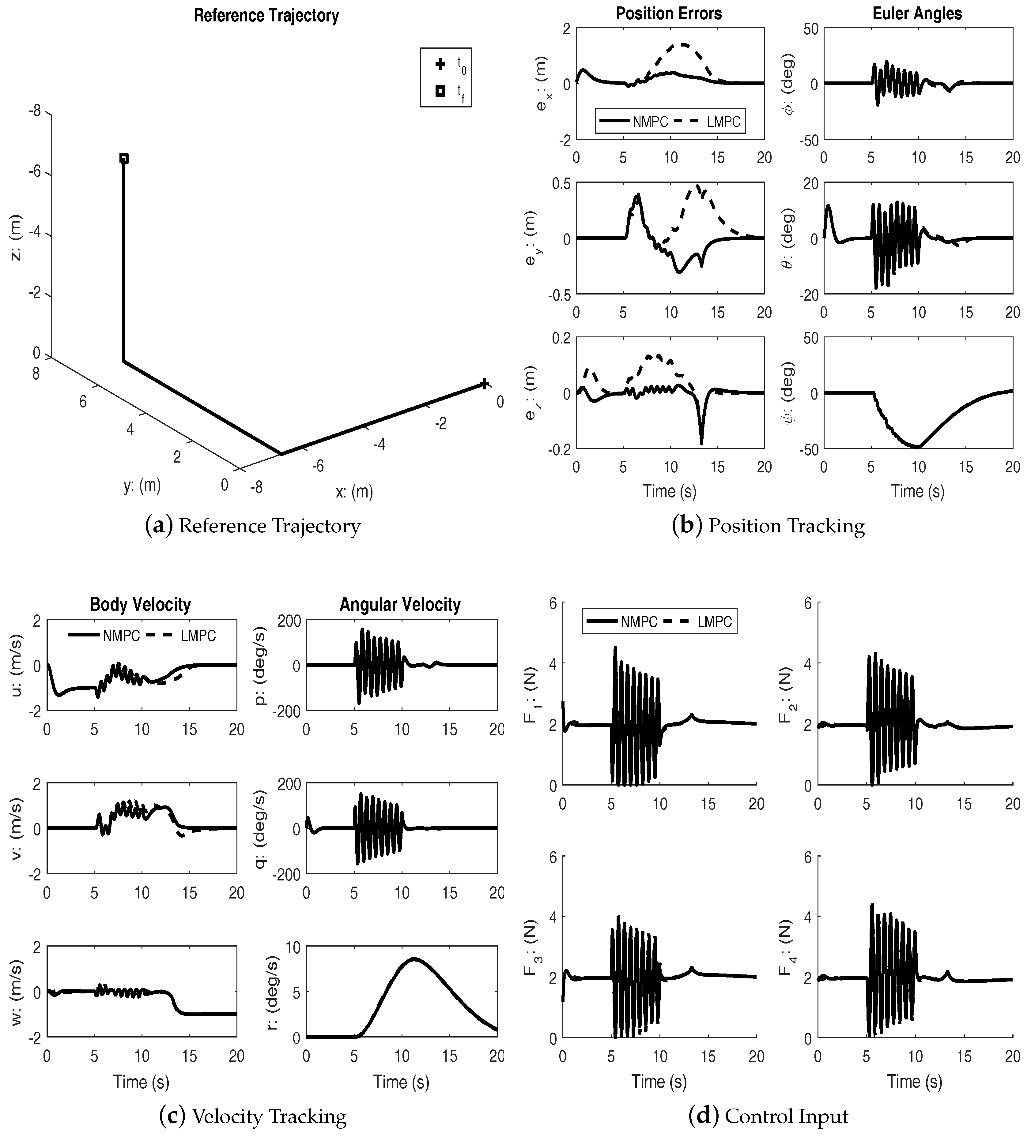
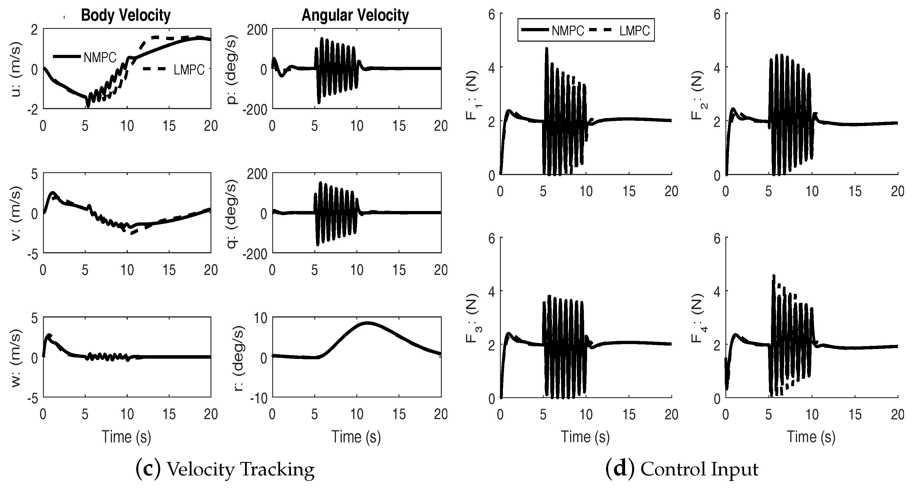
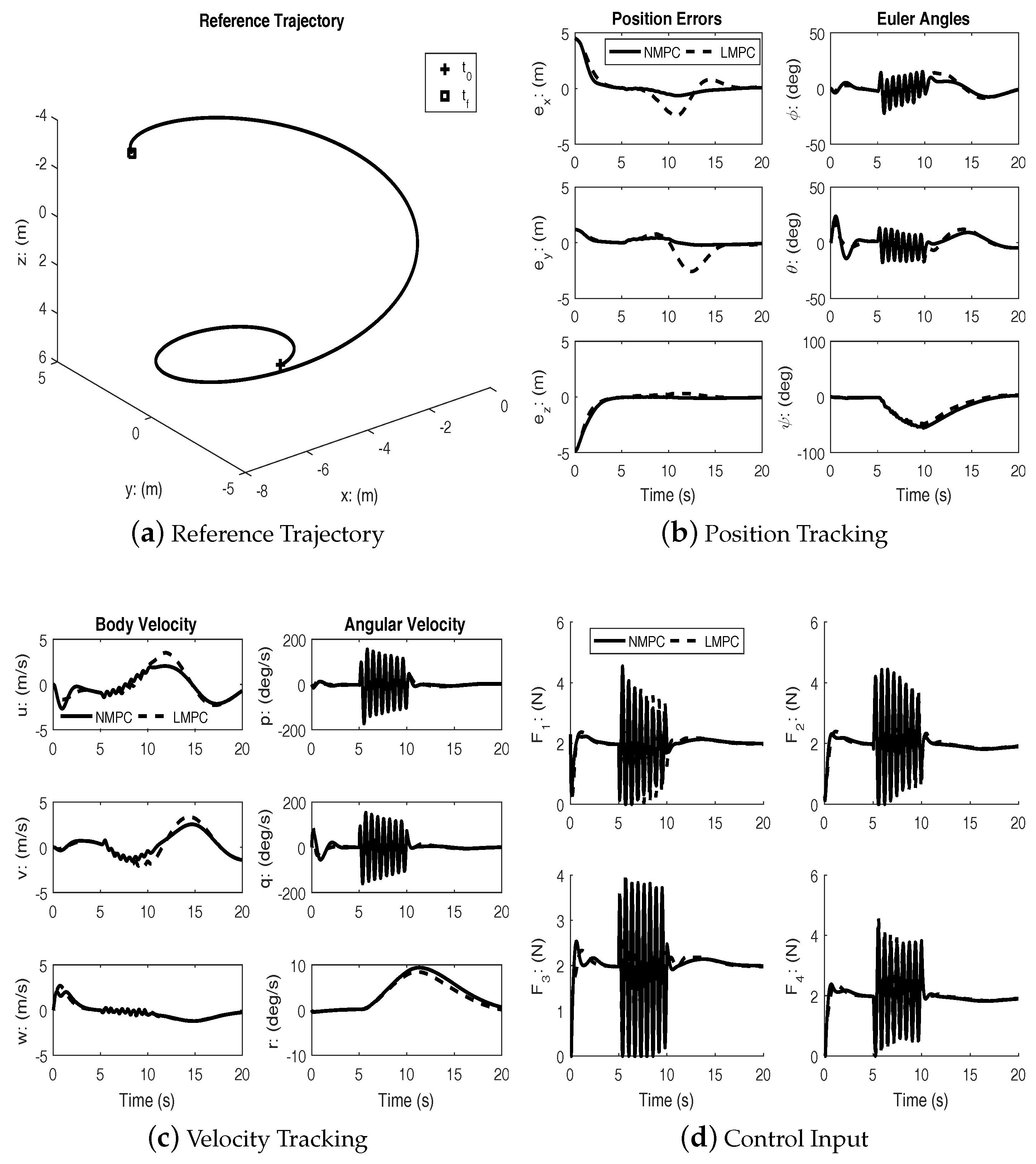
For both cases, the true system dynamics presented in Equation (51) along with the first order actuator dynamics for the rotor thrusts is simulated. Three different reference trajectories are generated to evaluate the effectiveness of the control laws: (a) helical, (b) spherical spiral and (c) straight line segments. The control input bounds are set as ${\mathbf{u}}_{lb}={\left[0000\right]}^T$ and ${\mathbf{u}}_{ub}={\left[mgmgmgmg\right]}^T$. The control horizon is chosen as $N=25$.

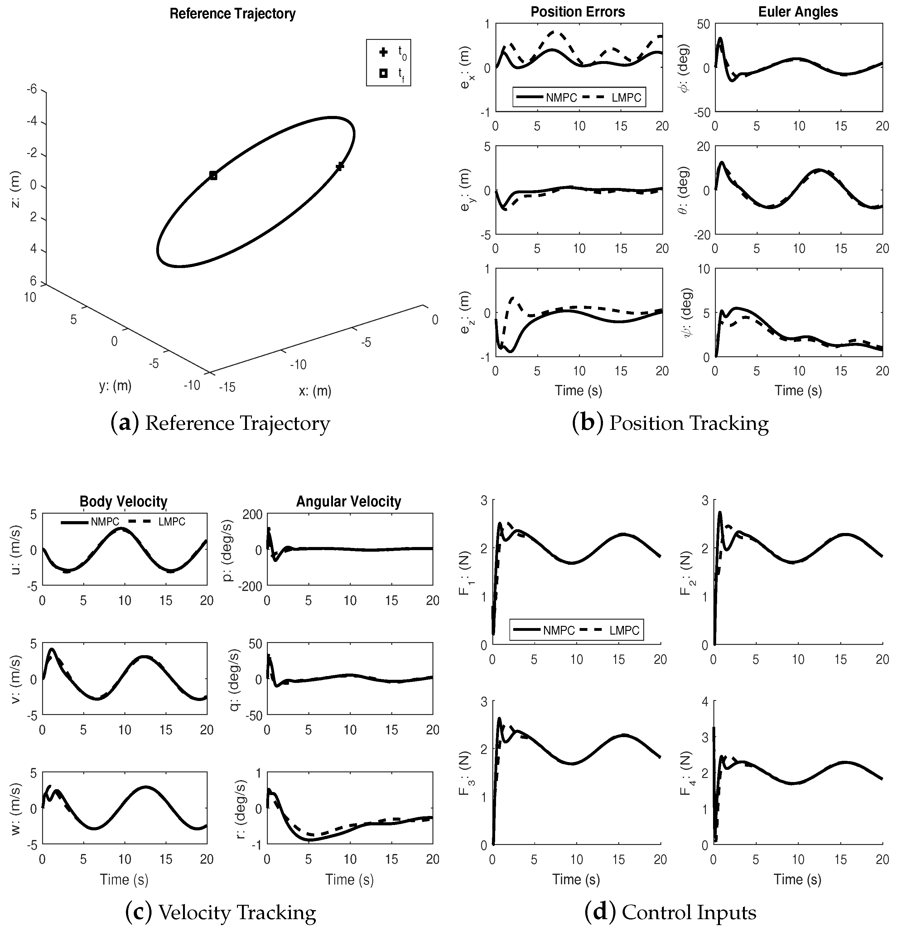
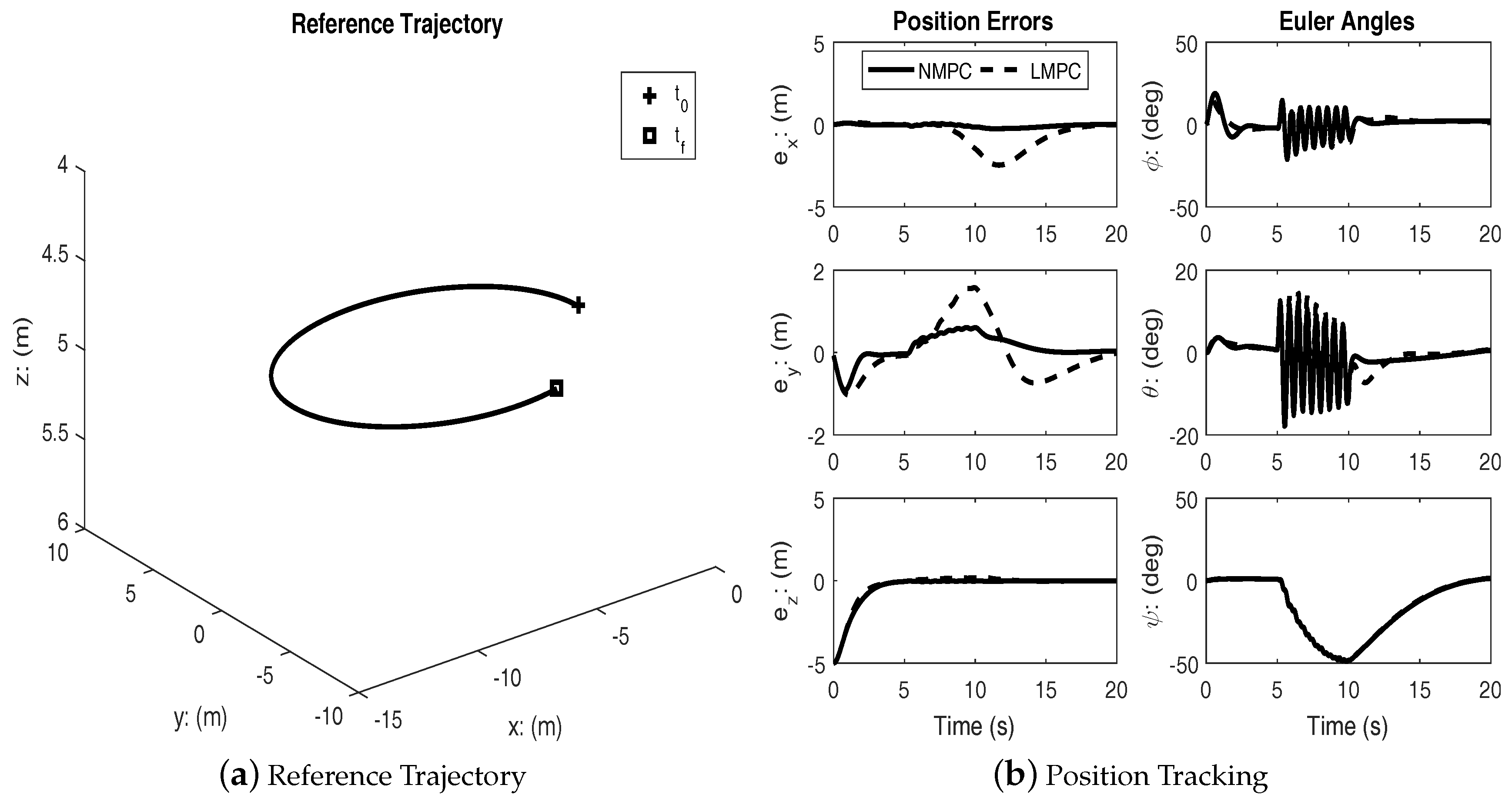
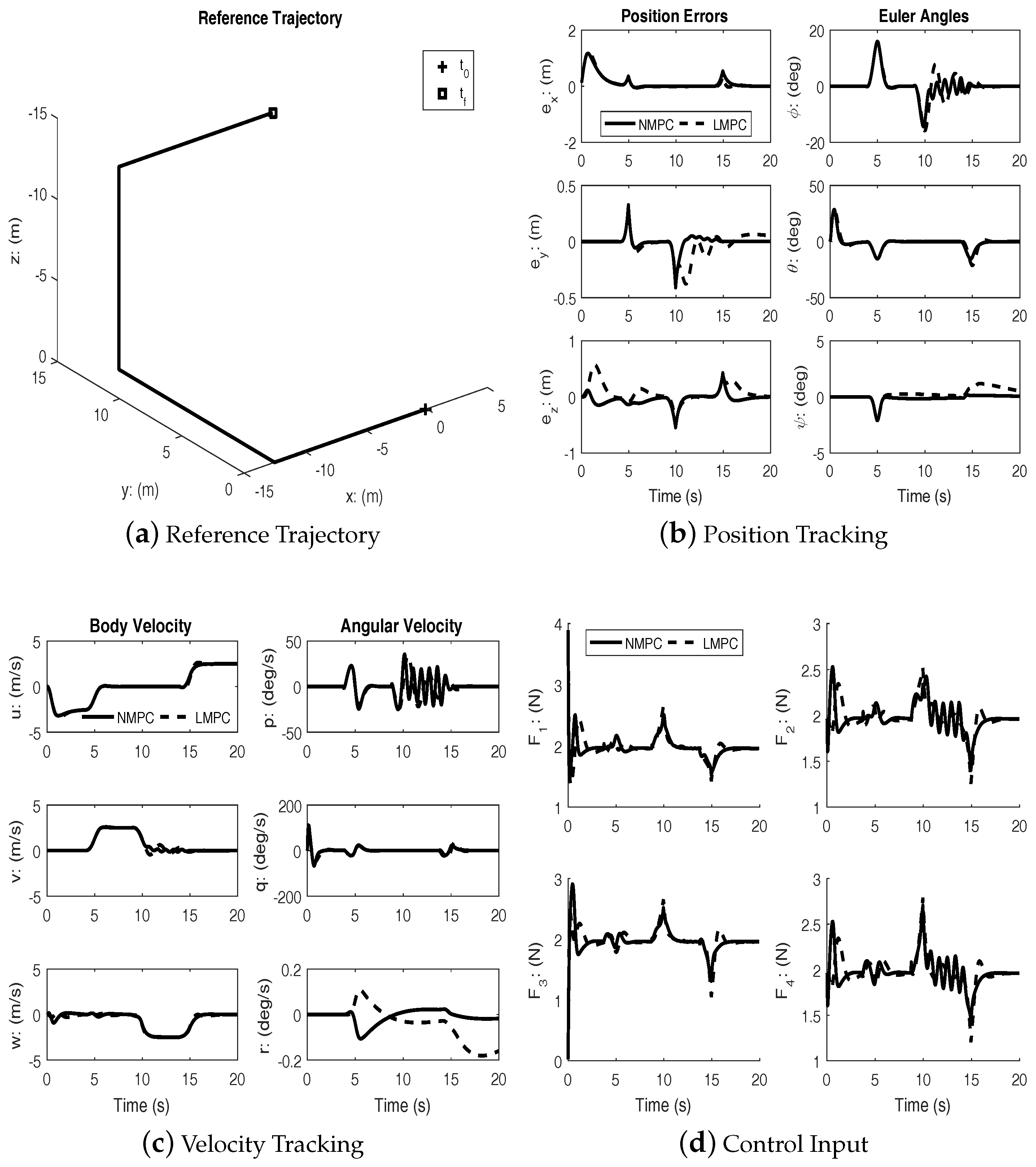
Figure 2 shows the reference trajectory and the tracking errors for both the linear and the nonlinear MPC cases. It can be seen that both controllers achieve good tracking; however, the transient response of the nonlinear MPC is better. Clearly, from Figure 2b, the speed of response with regards to tracking the position errors is much better for the nonlinear MPC.

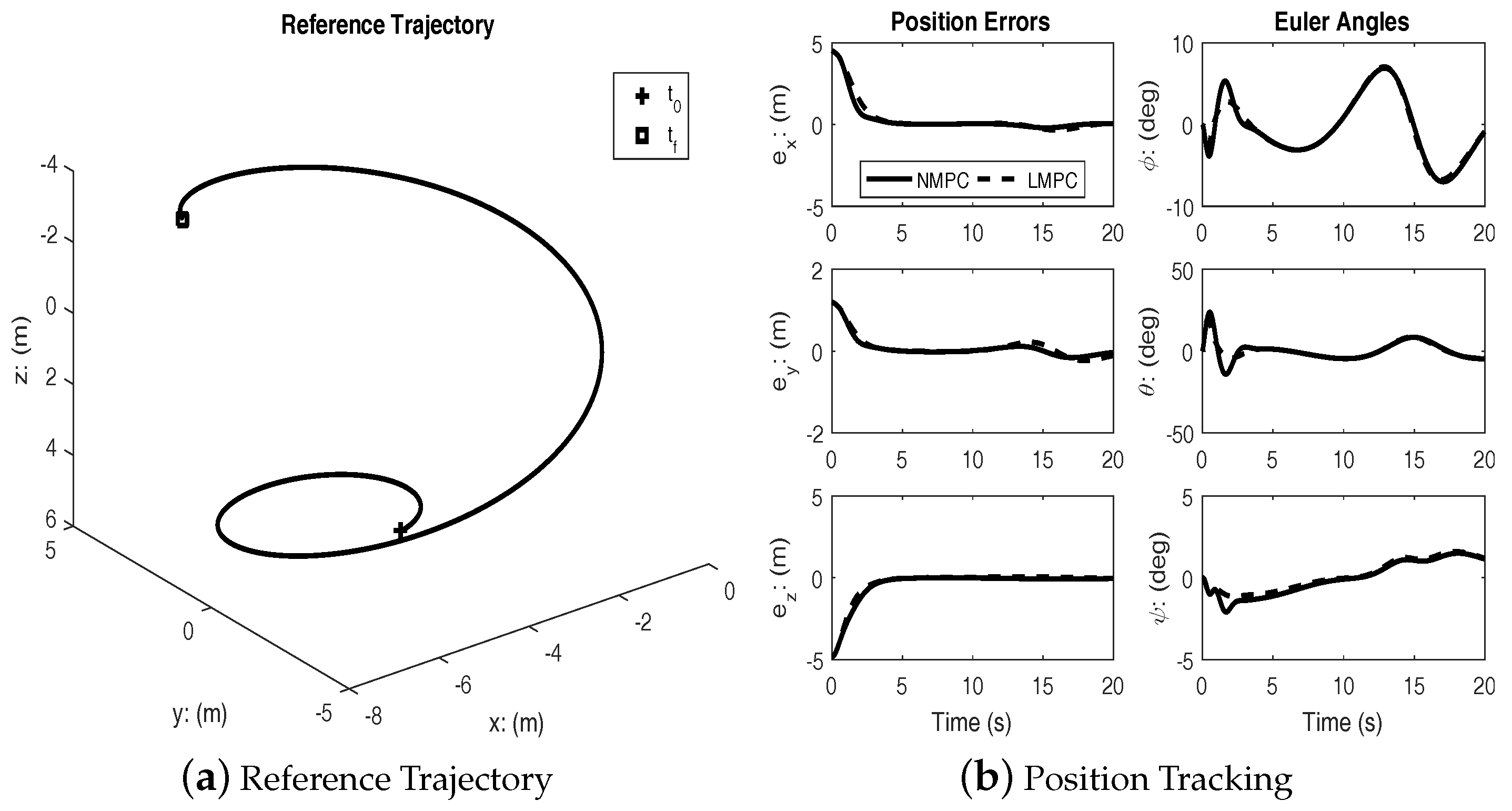
Figure 3 shows the results of tracking a spherical spiral trajectory. As with the previous case, both controllers achieve successful tracking.

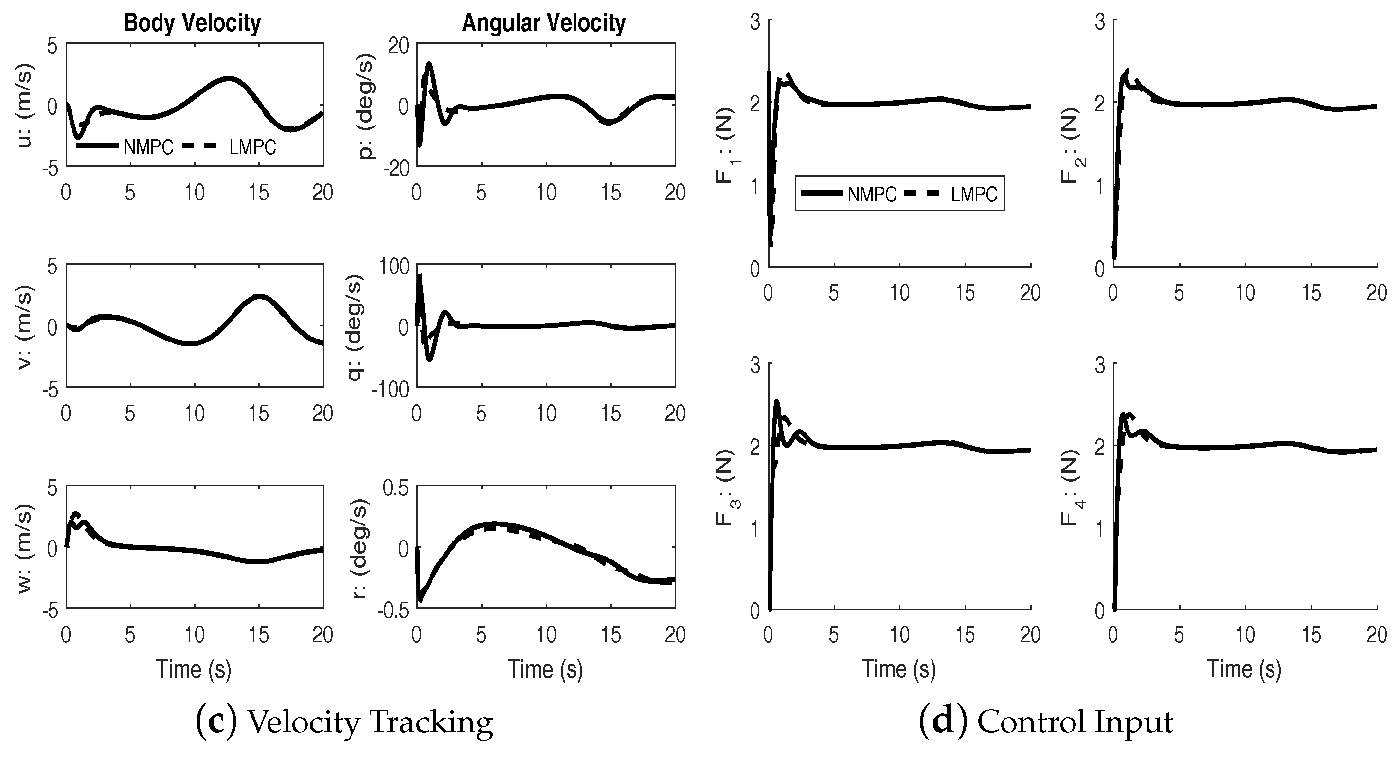
Figure 4 shows the results of tracking a straight line trajectory segment between two way points. As with the previous cases, both controllers achieve successful tracking. In this case, too, the superior transient performance of the nonlinear MPC is clearly seen. Additional studies show that the nonlinear MPC is able to track the trajectories even with a shorter prediction horizon.

Table 1. RMS of position tracking errors.

Trajectory	Nonlinear/Linear	N = 10	N = 15	N = 25	N = 35	N = 45
Helical	Nonlinear	0.5663	0.5824	0.5831	0.5757	0.5832
Helical	Linear	0.8075	0.8348	0.8484	0.8364	0.8334
Spherical Spiral	Nonlinear	1.4739	1.4725	1.4725	1.4720	1.4726
Spherical Spiral	Linear	1.4984	1.5000	1.5016	1.5009	1.5009
Straight Line	Nonlinear	0.3112	0.3020	0.3169	0.3160	0.3155
Straight Line	Linear	0.3722	0.3575	0.3633	0.3612	0.3603

showed the average root mean square (RMS) of position tracking errors of different prediction horizons. It can be seen that NMPC has better tracking performances in terms of position tracking.

Table 2. Average control effort ($\Delta {\mathbf{u}}^T\Delta \mathbf{u}$).

Trajectory	Nonlinear/Linear	N = 10	N = 15	N = 25	N = 35	N = 45
Helical	Nonlinear	0.3838	0.3724	0.3652	0.3665	0.3674
Helical	Linear	0.4205	0.4107	0.4057	0.4084	0.4114
Spherical Spiral	Nonlinear	0.1687	0.1689	0.1700	0.1707	0.1710
Spherical Spiral	Linear	0.1910	0.1913	0.1914	0.1913	0.1913
Straight Line	Nonlinear	0.2125	0.1433	0.1282	0.1280	0.1296
Straight Line	Linear	0.2245	0.1593	0.1388	0.1379	0.1367

showed the average control effort used in each tracking scenarios for different control horizons. In all three cases, NMPC is able to achieve better tracking with less control effort.

Nonlinear Model Predictive Control with Disturbance

In order to further assess the effectiveness of the NMPC scheme, simulations were performed with simultaneous high frequency disturbance torques injected in the roll and pitch channels. The disturbances are two exponentially decaying sinusoidal functions: $\delta \tau =e^{-0.1t}[sin\left(10t\right);cos\left(10t\right);0]$ during $t\in (5,10)\left(s\right)$. Figure 5, Figure 6 and Figure 7 show the performance of linear and nonlinear MPC subject to disturbance. The disturbance is used to approximate the effects of wind during typical outdoor flight conditions.

Under disturbances, linear MPC and nonlinear MPC both performed well with an acceptable amount of tracking errors and kept the input within bounds. It can be seen from the figures that the nonlinear MPC significantly out-performs the linear MPC with regards to transient performance.

7. Summary and Conclusions

A linear and nonlinear model predictive control scheme were presented to control a quadrotor platform with an objective to track various reference trajectories. The nonlinear model predictive controller made use of a state-dependent coefficient representation of the nonlinear dynamics that accounted for the peculiarities of the platform under consideration. The closed loop stability analysis of the linear and nonlinear control schemes were presented to show the similarities, as well as to highlight the differences. The nonlinear controller clearly outperformed the linear controller with superior transient performance in both nominal conditions and in the presence of high frequency disturbance torques in the roll and pitch channels.