
On a Non-Symmetric Eigenvalue Problem Governing Interior Structural–Acoustic Vibrations

Institute of Mathematics, Hamburg University of Technology, Am Schwarzenberg Campus 1, Hamburg D-21071, Germany
Aerospace 2016, 3(2), 17; https://doi.org/10.3390/aerospace3020017
Submission received: 22 April 2016
/
Revised: 30 May 2016
/
Accepted: 3 June 2016
/
Published: 17 June 2016
(This article belongs to the Special Issue Fluid-Structure Interactions)
Abstract
:Small amplitude vibrations of a structure completely filled with a fluid are considered. Describing the structure by displacements and the fluid by its pressure field, the free vibrations are governed by a non-self-adjoint eigenvalue problem. This survey reports on a framework for taking advantage of the structure of the non-symmetric eigenvalue problem allowing for a variational characterization of its eigenvalues. Structure-preserving iterative projection methods of the the Arnoldi and of the Jacobi–Davidson type and an automated multi-level sub-structuring method are reviewed. The reliability and efficiency of the methods are demonstrated by a numerical example.
1. Introduction
In this survey, we consider the free vibrations of an elastic structure coupled with an internal fluid. Such multi-physics problems arise in a wide variety of applications, such as the analysis of acoustic simulations of passenger car bodies, the response of piping systems and liquid or gas storage tanks and the simulation of the mechanical vibrations of ships and off-shore constructions, to name just a few. We restrict ourselves here to the elastoacoustic vibration problem, which consists of determining the small amplitude vibration modes of an elastic structure coupled with an internal inviscid, homogeneous, compressible fluid, where we neglect gravity effects.
The interaction between the structure and the fluid can significantly affect the response of the whole system and has to be taken into account properly. Different formulations have been proposed to solve this problem. One of them, the pure displacement formulation [1], has an attractive feature: it leads to a simple symmetric eigenvalue problem. However, due to the inappropriate treatment of the irrotationality condition, it suffers from the presence of zero-frequency spurious circulation modes with no physical meaning, and after discretization by standard finite elements, these modes correspond to nonzero eigenfrequencies commingled with physical ones.
In order to remove the problem with non-physical modes, a potential description consists of modeling the fluid by the pressure field p and the structure by the displacement field u (cf. [2,3,4,5,6,7]). Thus, one arrives at a non-self-adjoint variational formulation of the problem, and a Rayleigh–Ritz projection (e.g., by a finite element method) yields a linear, but non-symmetric matrix eigenvalue problem. This formulation has the advantage that it is smaller than the one from the pure displacement model, since it introduces only one unknown per node to describe the fluid, but it seems to be undesirable because eigensolvers for non-symmetric matrices, such as Arnoldi’s method, require a much higher cost than symmetric eigensolvers, both in terms of storage and computation.
Symmetric models of coupled fluid–structure vibration problems without spurious solutions have been achieved by describing the structural–acoustic system by a three field formulation complementing the structural displacement and the fluid pressure with the fluid velocity potential [8,9], or the vorticity moment [10], or the fluid displacement potential [11,12]. Finite element approximations based on this type of modeling are favored today, since one obtains symmetric matrix eigenvalue problems, and hence, variational characterizations of eigenvalues allow for using standard spectral approximation theory (see Babuska and Osborne [13]) to obtain convergence results for eigenvalues and eigenvectors for Galerkin-type projection methods (cf. [14,15,16,17,18]).
In this survey, we consider the elastoacoustic vibration problem describing the fluid by its pressure field and the structure by its displacement field. We prove that although the resulting eigenvalue problem is non-self-adjoint, it shares many important properties with the symmetric model: taking advantage of a Rayleigh functional (which generalizes the Rayleigh quotient for self-adjoint problems), its eigenvalues allow for the variational characterizations known from the symmetric theory. Namely, they can be characterized by Rayleigh’s principle and are minmax and maxmin values of the Rayleigh functional.
The paper is organized as follows. Section 2 introduces the fluid–solid interaction problem and collects some of its properties, in particular a relation between left and right eigenfunctions corresponding to the same eigenvalue, which motivate in Section 3 the definition of a Rayleigh functional. We summarize variational characterizations of its eigenvalues generalizing Rayleigh’s principle and the minmax and maxmin characterizations known for self-adjoint problems. Section 4 demonstrates that a common approach to neglect the coupling of the structure and the fluid yields unsatisfactory approximations at least in the case of strong coupling. Section 5 is devoted to the structure-preserving iterative projection methods of the nonlinear Arnoldi and the Jacobi–Davidson type. In Section 6, we outline a generalization of the automated multi-level sub-structuring method. The efficiency of these approaches is demonstrated by a numerical example. The paper closes with concluding remarks.
2. Structural–Acoustic Vibrations
We consider the free vibrations of an elastic structure completely filled with a homogeneous, inviscid and compressible fluid neglecting gravity effects. The fluid and the solid occupy Lipschitz domains and , respectively, which we assume non-overlapping, .
We assume the boundary to be divided:
into pairwise disjoint parts , where and are Dirichlet- and Neumann-type boundaries and is a common interface, which is responsible for the coupling effect. The linear-elastic solid is modeled by its displacement function , . The incompressible, inviscid and homogeneous fluid is described by the relative pressure . This yields a formulation as a system of homogeneous time-independent partial differential equations:
where ω is the eigenfrequency of vibrations, σ is the stress tensor of the solid, is the unit normal vector on and n denotes the unit normal vector on oriented towards the solid part. The interface boundary conditions are a consequence of an equilibrium of acceleration and force densities at the contact interface. We assume that the fluid density is constant in and that the solid density satisfies where and (as in the whole paper) denote positive generic constants.
The variational form can be obtained separately for the solid and the fluid. For some bounded domain , appropriate function spaces are given by the Sobolev spaces:
endowed with the scalar product:
where the derivatives are meant in the weak sense. To take into account homogeneous Dirichlet boundary conditions, we introduce the space for as the completion of in , where denotes the space of infinitely often differentiable functions u on Ω with in a neighborhood of Γ.
To rewrite the problem in a variational formulation, we define the bilinear forms:
where denotes the scalar matrix product. Then, we obtain the following problem.
Find and nonzero , such that:
for all .
Note that and are continuous in and . For the linearized strain tensor ϵ in the solid, we assume that the strain–stress relationship satisfies:
for some constant , such that Korn’s second inequality implies that is a coercive bilinear form.
Equation (2) can be written in operator notation. The aim is to find and nonzero so that:
where the operators are defined corresponding to the variational formulation in Equation (2).
The following Lemma collects some elementary properties of the fluid–solid interaction eigenvalue problem and its adjoint problem:
Find and nonzero , such that:
for all .
Lemma 1.
- (i)
- The eigenvalue problem and its adjoint problem have a zero eigenvalue with corresponding one-dimensional eigenspaces and where , and is the unique solution of the variational problem for every .
- (ii)
- The function is an eigensolution of the right eigenvalue problem corresponding to an eigenvalue if and only if is an eigensolution of the adjoint eigenvalue problem corresponding to the same eigenvalue.
- (iii)
- Eigenfunctions and of Problem (2) corresponding to distinct eigenvalues are orthogonal with respect to the inner product:
- (iv)
- Assume that is an eigensolution of Problem (2) and an eigensolution of the adjoint Problem (4) corresponding to the eigenvalues and , respectively.If , then it holds that:If and , then it holds that:
- (v)
- The eigenvalue Problem (2) has only real nonnegative eigenvalues, the only accumulation point of which is ∞.
Proof.
cf. [19], Lemma 3.1. ☐
3. Variational Characterizations of Eigenvalues
For a wide class of linear self-adjoint operators , a Hilbert space, the eigenvalues of the linear eigenvalue problem can be characterized by three fundamental variational principles, namely by Rayleigh’s principle [20], by Poincaré’s minmax characterization [21] and by the maxmin principle of Courant [22], Fischer [23] and Weyl [24]. These variational characterizations of eigenvalues are known to be very powerful tools when studying self-adjoint linear operators on a Hilbert space . Bounds for eigenvalues, comparison theorems, interlacing results and the monotonicity of eigenvalues can be proven easily with these characterizations, to name just a few. We now take advantage of the generalizations of these principles to nonlinear eigenvalue problems.
Lemma 1 states the relationship between eigenfunctions of Problem (2) and its adjoint Problem (4). The adjoint eigenfunction can be used as a test function in Equation (2), so that we obtain:
for any eigensolution of Problem (2), i.e., the eigenvalue λ is a zero of the function:
If , this equation is quadratic in λ. In any case, it can be shown [19] (Lemma 4.1) that if is an eigenfunction of Problem (2), the maximal root of Equation (5) is the nonnegative eigenvalue of Problem (2) corresponding to . This suggests introducing an eigenvalue approximation for some general nonzero by g, and we define the nonlinear Rayleigh functional as the maximal root of .
Definition 2.
The functional , where any nonzero is mapped to the maximal root of is called the nonlinear Rayleigh functional, i.e.,
where:
Although the fluid–solid eigenvalue problem is not self-adjoint, its Rayleigh functional shares many properties with the one of self-adjoint problems.
Theorem 3.
Every eigenelement of Problem (2) is a stationary point of r, i.e.,
Proof.
cf. [25], Theorem 4.1. ☐
Moreover, using the nonlinear Rayleigh functional, one obtains the following variational characterizations, which generalize the variational principles known for the linear self-adjoint [20,21,22,23,24] and for the nonlinear self-adjoint case [26,27].
Theorem 4.
Let be the eigenvalues of Problem (2) in ascending order and corresponding eigenfunctions. Then, it holds that:
- (i)
- (Rayleigh’s principle)
- (ii)
- (minmax characterization)
- (iii)
- (maxmin characterization)where:
Proof.
cf. [19], Theorem 4.1. ☐
From the minmax characterization, we immediately obtain the following comparison result: if is a subspace of , then the eigenvalues of the projection of Problem (2) to V are upper bounds of the corresponding eigenvalues of Problem (2), and this is in particular true for a discretization by a projection method (e.g., a finite element method) or for the eigenvalues of the decoupled structure part or the fluid part of the problem.
Remark 1.
There are further variational characterizations of the eigenvalues of the linear, non-self-adjoint eigenvalue Problem (2). It can be rewritten as a quadratic and self-adjoint problem, which also allows for a variational characterization of its eigenvalues. Substituting and , one obtains from Equation (2) after dividing the second equation by ω:
where the occurring operators again are defined corresponding to the variational formulation in Equation (2).
Testing Equation (10) with , one obtains the quadratic equation:
which for every has a unique positive solution . Hence, the quadratic eigenvalue Problem (10) also defines a functional , which is also called Rayleigh functional, and the eigenvalues of Equation (2) can be characterized by variational characterizations, which read exactly as in Theorem 4; we only have to replace the Rayleigh functional r with (cf. [26,27,28,29]).
Remark 2.
If λ is not contained in the spectrum of the eigenvalue Problem (12), then we obtain from the first equation of Equation (2) , and the fluid pressure p is a solution of the rational eigenvalue problem:
Equation (13) is not defined if λ equals one of the , but for each of the intervals , all eigenvalues can be characterized by a minmax characterization [30,31]. Notice, however, that in this case, one cannot use the natural enumeration, but the numbering of the eigenvalues requires a certain adjustment to the interval .
4. Discretization by Finite Elements
Galerkin methods for Problem (1) consist of replacing the infinite dimensional space by some finite dimensional space . The finite element method is a Galerkin method where consists of piecewise polynomials. In the sequel, we assume that the solid and the fluid domains are discretized separately, such that the resulting finite element spaces are compatible on the interface boundary, i.e., for each , there exists a , such that on in the weak sense.
We assume that we have nodal bases of and whose elements are denoted by and , and let s and f be the dimensions of the solid and fluid function spaces and , respectively. Then, restricting Problem (2) to , we obtain the following discretized problem:
Find and , such that:
for all .
Since is finite dimensional, we can write Equation (14) as a matrix eigenvalue problem. With sparse matrices:
we obtain the non-symmetric problem: find and , such that:
Clearly, this problem inherits from the infinite dimensional Problem (1) that all eigenvalues are real and nonnegative, that they allow for the variational characterizations in Theorem 4 (where and have to replaced by and , respectively) and that the orthogonality properties in Lemma 1 (iii) hold, i.e., if , are eigenvectors of Equation (15) corresponding to distinct eigenvalues, then it holds:
Moreover, eigenvalues of the discrete Problem (15) are upper bounds of the corresponding eigenvalues of the infinite dimensional Problem (2).
Due to lacking symmetry, the computational solution of Equation (15) with standard sparse eigensolvers involves considerable complications. Krylov-type solvers like the Arnoldi method or rational Krylov approaches require long recurrences when constructing the projection to a Krylov space and, therefore, a large amount of storage. Moreover, general iterative projection methods destroy the structure of Equation (15) and may result in non-real eigenvalues and eigenvectors, and then, they require complex arithmetic.
As a remedy, some authors prefer an alternative modeling, which additionally involves the fluid displacement potential. Then, the resulting system is symmetric, and efficient methods, such as the shift-and-invert Lanczos method apply (e.g., [14,15,16,17,18]). As a drawback, however, the dimension of the problem increases considerably.
A common approach for solving Equation (15) (for example, in the automotive industry, e.g., [32,33,34]), which works fine for weakly-coupled systems, is as follows: one first determines the eigenpairs of the symmetric and definite eigenvalue problems:
by the Lanczos method or by automated multi-level sub-structuring (AMLS) ([34,35,36]) and then one projects Equation (15) to the subspace spanned by and , where the columns of and are the eigenmodes of Equation (17), the corresponding eigenvalues of which do not exceed a given cut-off level. The projected problem:
has the same structure as the original problem, but is of much smaller dimension and can then be treated with the common solvers, like the Arnoldi method at justifiable cost. The eigenvalues of Equation (18) are upper bounds of the corresponding eigenvalues of Equation (15) and of the infinite dimensional Problem (1).
The following example demonstrates that this approach is not appropriate for strongly-coupled problems:
Example 1.
We first consider a two-dimensional coupled structure (the geometry is shown in Figure 1) consisting of steel and air portions. We chose a very large interface between the fluid and the structure to accent the coupling effect.
We discretized by quadratic Lagrangian elements on a triangular grid. The resulting problem has 120,473 degrees of freedom, 67,616 of which are located in the solid region and 52,857 in the fluid part.
Table 1 contains in its first column the 10 smallest eigenfrequencies of the coupled problem and in its second and third columns the eigenfrequencies of and , respectively, demonstrating that each eigenfrequency of the coupled system can be assigned in an obvious way to an eigenfrequency of one of the portions. Hence, the coupling has only marginal influence. Column 4 shows the relative deviations (marked as Rel. Dev.) in % of the eigenfrequencies of the coupled and the uncoupled system.
Projecting the coupled problem to the space spanned by the eigenmodes of the individual problems in Equation (17), the eigenfrequencies of which do not exceed 1000 Hz, the relative errors in % are even reduced to less than (cf. column 5 of Table 1 marked as Rel. Err. Proj.).
If the fluid air is replaced by water, the scene changes completely. Table 2 contains in its first column the 10 smallest eigenvalues of the coupled structure and in Columns 2 and 3, the smallest eigenvalues of the steel and the water portion, respectively, and there is no obvious correspondence of the eigenvalues of the coupled system to a structure or a fluid eigenvalue.
Again, we projected the coupled problem to the space spanned by the eigenmodes of the problems in Equation (17), the eigenfrequencies of which do not exceed 1000 Hz. The 10 smallest eigenfrequencies of the projected problem (marked as Proj.) are shown in column 4, and the relative errors in % (marked as Rel. Err.) in column 5 demonstrating that the approximations to the correct eigenvalues are not satisfactory.
5. Structure Preserving Numerical Methods
For symmetric eigenvalue problems, the Rayleigh quotient iteration converges cubically to simple eigenvalues. For non-symmetric problems, the convergence is only quadratic. However, if for the structural–acoustic eigenvalue Problem (1) the Rayleigh quotient is replaced by the Rayleigh functional r, then taking advantage of the stationarity of r at eigenelements, the Rayleigh functional iteration Algorithm 1 can also be shown to be cubically convergent (cf. [25]).
| Algorithm 1 Rayleigh functional iteration for fluid–solid eigenvalue problems. |
Require: initial vector
|
Rayleigh functional iteration converges fast, but often, it is highly sensitive with respect to initial vectors. The basin of attraction can be very small, and an erratic behavior of the iteration can be observed. To avoid the possible failure of the Rayleigh functional iteration, one combines it with an iterative projection method, which has proven to be very efficient.
5.1. Structure-Preserving Iterative Projection Methods
We now present structure preserving iterative projection methods for the non-symmetric eigenvalue Equation (15) that allows for taking into account also strong coupling of fluid–solid structures in the analysis and numerical solution of free vibrations.
An iterative projection method works as follows. It starts with a subspace to which the given problem is projected. The dimension of the projected eigenproblem is usually very small, and therefore, it can be solved by a standard eigensolver, and an approximation to a wanted eigenvalue and a corresponding eigenvector can be extracted.
This eigenpair is accepted if it meets specified accuracy requirements; otherwise, the space is expanded by a new direction. Methods of this type are Krylov subspace methods, like the Lanczos method, the Arnoldi method, or rational Krylov methods, and Davidson or Jacobi–Davidson type methods (cf. [37]). The idea of iterative projection methods is that search spaces are able to capture the essential structure of the original problem if the expanding directions are chosen appropriately, and then, the dimension of the search space can be kept small.
If is a basis of a search space , the projection of Equation (15) reads
Hence, the structure of Equation (15) gets lost, and it is not certain that eigenvalues of the projected problem stay real.
This suggests to use an ansatz space in a structure-preserving projection method, i.e., to project the mass part and the fluid part of the problem individually to search spaces. Then, the projected problem receives the form Equation (18), and the eigenvalues of the projected problem stay real. From Theorem 4, it follows that the eigenvalues of the projected problem are upper bounds of the eigenvalues of the original Equation (15), and expanding the search space, all eigenvalues decrease and (hopefully) get better approximations to the eigenvalues of Equation (15).
An expansion with high approximation potential is given by the Rayleigh quotient iteration, i.e., if is a (orthonormal) basis of the current search space and is an eigenpair of the projected problem:
a reasonable expansion of the search space is the solution v of the linear system:
where denotes the Ritz vector corresponding to .
In the course of the algorithm, the approximation θ to an eigenvalue λ changes in every step, and therefore, large-scale linear systems with varying system matrices have to be solved in consecutive iteration steps, which is much too costly for truly large problems.
To remedy this drawback, we reformulate the expansion of . We take advantage of the fact that for every , the solution of Equation (20) satisfies:
and that the current Ritz vector x is already contained in . Hence, , where denotes the generalized Cayley transformation:
Hence, the expansion of requires the solution of a linear system , where the system matrix can be kept fixed for several iteration steps.
We obtain Algorithm 2, where we even replace by a preconditioner, since for truly large problems, it is too costly to solve the linear system exactly. This method was introduced in [38] for nonlinear eigenvalue problems, and since it reduces for general linear eigenvalue problems to the inexact shift-and-invert Arnoldi method, it was called nonlinear Arnoldi method.
Some comments are in order:
- (i)
- Since the dimension of the projected eigenproblem is quite small, it is solved by a dense solver, and therefore, approximations to further eigenpairs are at hand without additional cost.
- (ii)
- In the inner while clause, we check whether approximations to further eigenpairs already satisfy the specified error tolerance. Moreover, at the end of the while-loop,an approximation to the next eigenpair to compute and the residual r are provided.
- (iii)
- If the dimension of the search space has become too large, we reduce the matrices and , such that the columns of the new (and ) form a (and )orthonormal basis of the space spanned by the structure and the fluid part of the eigenvectors found so far. Notice that the search space is reduced only after an eigenpair has converged because the reduction spoils too much information, and the convergence can be retarded.
- (iv)
- The preconditioner is chosen, such that a linear system can be solved easily, for instance as a (incomplete) Cholesky or (incomplete) LU factorization. It is updated if the convergence measured by the reduction of the residual norm has become too slow.
- (v)
- It may happen that a correction t is mainly concentrated on the structure and the fluid, respectively, and the part of the complementary structure is very small. In this case, we do not expand in Step 22 and in Step 19, respectively.
- (vi)
A different approach for expanding the search spaces, which is also based on the Rayleigh quotient iteration, was also considered in [25]. At least close to an eigenpair, the expansion is very sensitive to inexact solving of the linear Equation (20).
In [40], it was shown that the most robust expansion of that contains the direction v of the Rayleigh functional iteration is where α is chosen, such that (for a definition of cf. Equation (16)), i.e.,
It is easily seen that t solves the correction equations:
which demonstrates that the resulting iterative projection method is a Jacobi–Davidson-type method [41].
| Algorithm 2 Structure-preserving nonlinear Arnoldi method for fluid–solid eigenvalue problems. |
|
The linear Equation (23), which looks even more complicated than Equation (20) cannot be solved by a direct solver, but has to be tackled by an iterative method, like the preconditioned GMRES method (Generalized Minimum RESidual method, cf. [42]). A natural choice for a preconditioner is:
where L is a reasonable preconditioner for .
It was observed already by Sleijpen and van der Vorst [43] that including the projectors and into the preconditioner does not increase the cost of preconditioned GMRES very much. Only one additional application of the preconditioner is necessary in every iteration step to initialize the inner iteration for solving Equation (23). The Jacobi–Davidson-type method for fluid–solid structures was introduced in [25], where it is discussed in detail.
The resulting Jacobi–Davidson method is nearly identical to Algorithm 2. We only have to replace Statement 16 by:
Find approximate solution of the correction Equation (23) (for instance, by a preconditioned Krylov solver).
5.2. Numerical Example
To evaluate the discussed iterative projection methods for the fluid–solid vibration problem, we consider Example 1, where the solid is steel and the fluid is water.
We determined all eigenvalues to be less than 500 Hz. Although we chose a (fixed) random initial vector, such that the initial Rayleigh functional was in the middle of the spectrum, the nonlinear Arnoldi method and the Jacobi–Davidson method determined the 10 wanted eigenvalues safely in all experiments, demonstrating the robustness of both methods.
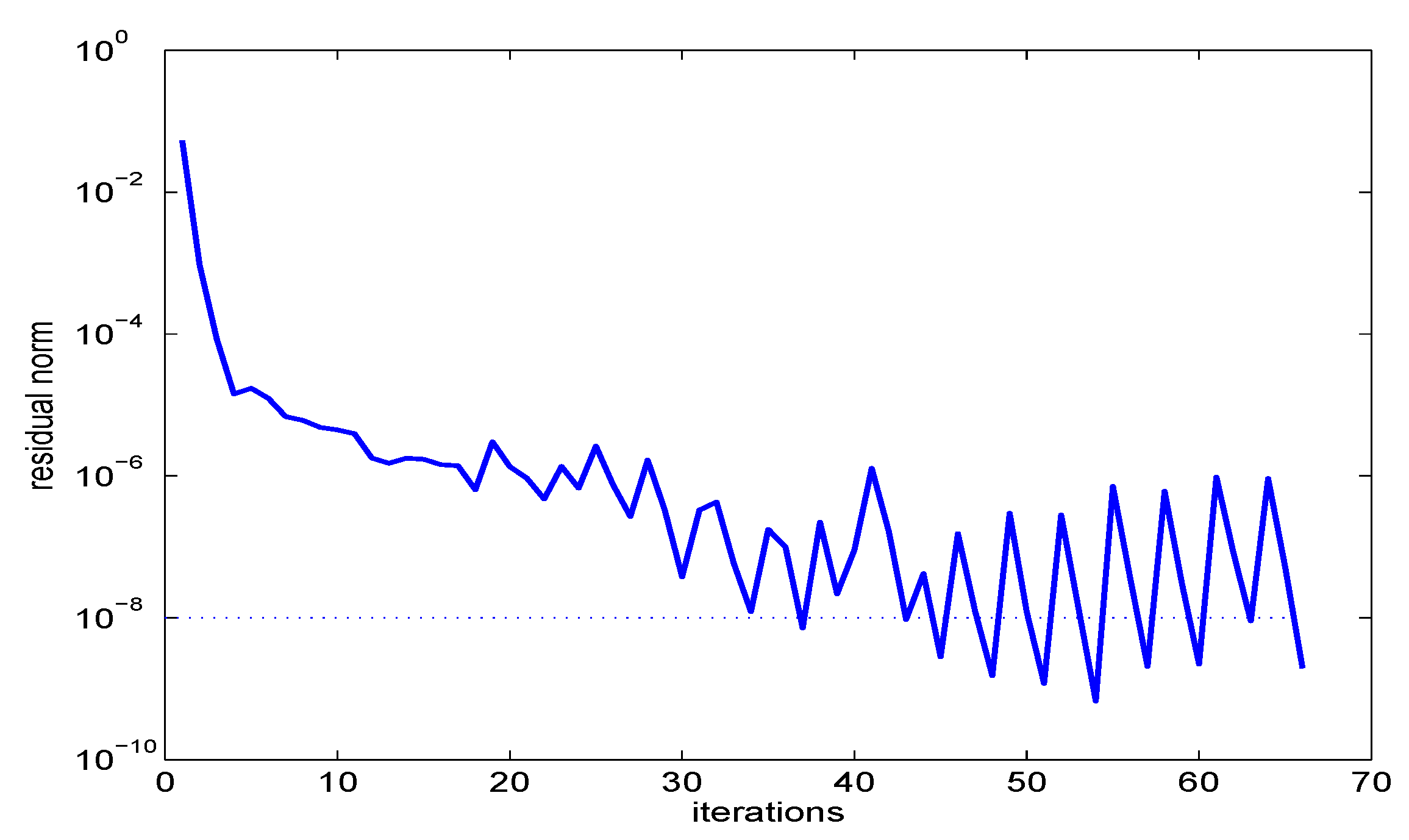
Using a very accurate preconditioner (named block Colesky preconditioner in Figure 2 and Figure 3), namely , where and denotes the Cholesky factor of and , respectively, the nonlinear Arnoldi method turned out to be faster than the Jacobi–Davidson method. On a Pentium D processor with 3.4 GHz and 4 GB RAM under MATLAB 2009, the nonlinear Arnoldi method required 10.4 s, whereas the Jacobi–Davidson method needed 30.0 s.
The convergence history is contained in Figure 2 for the nonlinear Arnoldi method and in Figure 3 for the Jacobi–Davidson method. These figures demonstrate that both methods required quite a large number of iterations to determine the smallest eigenvalue (namely, 15 iterations for the nonlinear Arnoldi and 10 iterations for the Jacobi–Davidson method), and then, each of the following eigenvalues was found after two or three iterations.
Notice that every step of the Jacobi–Davidson method requires the approximate solution of a linear system, whereas in the nonlinear Arnoldi method, one only has to apply the preconditioner ones. Hence, the CPU time needed by the nonlinear Arnoldi method is much smaller, although it requires a larger number of iteration steps than the Jacobi–Davidson method.
Replacing the block Cholesky factorization by an incomplete LU factorization of (cf. [42]), the CPU time needed by the Jacobi–Davidson method increases to 60.5 s if the cut-off threshold is chosen to be and 113.4 s for , whereas the nonlinear Arnoldi method requires 125.6 s and 3411.1 s, respectively. The convergence histories are displayed in Figure 4 and Figure 5.
This behavior was already observed for general nonlinear eigenvalue problems. If an accurate preconditioner is available, then the nonlinear Arnoldi method is usually much faster than the Jacobi–Davidson method. However, the Jacobi–Davidson method is much more robust with regard to coarse preconditioners.
6. Automated Multi-Level Sub-Structuring
6.1. Automated Multi-Level Sub-Structuring for Hermitian Problems
Over the last twenty years, a new method for huge linear eigenvalue problems:
where and are Hermitian and positive definite, known as automated multi-level sub-structuring (AMLS), has been developed by Bennighof and co-authors and has been applied to frequency response analysis of complex structures [34,35,36,44,45,46,47]. Here, the large finite element model is recursively divided into very many sub-structures on several levels based on the sparsity structure of the system matrices. Assuming that the interior degrees of freedom of sub-structures depend quasistatically on the interface degrees of freedom and modeling the deviation from quasistatic dependence in terms of a small number of selected sub-structure eigenmodes, the size of the finite element model is reduced substantially, yet yielding satisfactory accuracy over a wide frequency range of interest.
Recent studies in vibro-acoustic analysis of passenger car bodies (e.g., [34,45]), where very large FE models with more than six million degrees of freedom appear and several hundreds of eigenfrequencies and eigenmodes are needed, have shown that for this type of problem, AMLS is considerably faster than Lanczos-type approaches.
We briefly sketch the component mode synthesis (CMS) method for the general linear eigenvalue problem , which is the essential building block of the AMLS method. CMS assumes that the graph of the matrix is partitioned into sub-structures. This can be done efficiently by graph partitioners, like METIS [48] or CHACO [49], based on the sparsity pattern of the matrices.
We distinguish only between local (i.e., interior) and interface degrees of freedom. Then, K and M (after reordering) have the following form:
where and are block diagonal.
Annihilating by block Gaussian elimination and transforming the local coordinates to modal degrees of freedom of the substructures, one obtains the equivalent pencil:
Here, Ω is a diagonal matrix containing the sub–structure eigenvalues, i.e., , and Φ contains in its columns the corresponding eigenvectors. In structural dynamics, Equation (28) is called the Craig–Bampton form of the eigenvalue Problem (26) corresponding to the partitioning in Equation (27).
Selecting some eigenmodes of the eigenvalue problem , usually the ones associated with eigenvalues below a cut-off threshold γ and dropping the rows and columns in Equation (28) corresponding to the other modes, one arrives at the component mode synthesis method (CMS) introduced by Hurty [50] and Craig and Bampton [51]. The corresponding matrices still have the structure given in Equation (28) with curtailed matrices.
For medium-sized eigenvalue problems, this approach is very efficient. Since and are block diagonal, it is quite inexpensive to eliminate and to solve the interior eigenproblems . However, with the increasing size of Problem (26), CMS suffers some drawbacks. Coarse partitioning leads to huge sub-structures, such that the decoupling and modal reduction become costly, whereas fine partitioning yields a large projected eigenvalue problem , which is dense, and therefore, its numerical solution is time consuming.
A remedy of this dilemma is the AMLS method, which generalizes CMS in the following way. Again, the graph of is partitioned into a small number of subgraphs, but more generally than in CMS, these subgraphs in turn are sub-structured on a number p of levels. This induces the following partitioning of the index set of degrees of freedom. is the set of indices corresponding to interface degrees of freedom on the coarsest level, and for , define to be the set of indices of interface degrees of freedom on the j-th level, which are not contained in . Finally, let be the set of interior degrees of freedom on the finest level.
With these notations, the first step of AMLS is CMS with cut-off frequency γ applied to the finest sub-structuring. After j steps, , one derives a reduced pencil:
where p denotes the degrees of freedom obtained in the spectral reduction in the previous steps, ℓ collects the indices in and i corresponds to the index set of interface degrees of freedom on levels that are not yet treated. Applying the CMS method to the southeast blocks of the matrices, i.e., annihilating the off–diagonal block by block Gaussian elimination and reducing the set of ℓ-indices by spectral truncation with cut-off frequency γ, one arrives at the next level. After p CMS steps and a final spectral truncation of the lower-right blocks, one obtains the reduction of Equation (26) by AMLS.
Hence, on each level of the hierarchical sub-structuring, AMLS consists of two steps. First, for every sub-structure of the current level, a congruence transformation is applied to the matrix pencil to decouple in the stiffness matrix the sub-structure from the degrees of freedom of higher levels. Secondly, the dimension of the problem is reduced by modal truncation of the corresponding diagonal blocks discarding eigenmodes according to eigenfrequencies, which exceed a predetermined cut-off frequency. Hence, AMLS is nothing but a projection method where the large problem under consideration is projected to a search space spanned by a smaller number of eigenmodes of clamped sub-structures on several levels.
AMLS must be implemented unlike the description above to ensure computational efficiency. Firstly, it is important to handle structures on the same partitioning level separately to profit from the decoupling. Furthermore, structures must be handled in an appropriate order. If all sub-structures that are connected to the same interface on the superior level have already be condensed, the interface should be reduced, as well, to avoid the storage of large dense matrices.
If all sub-structures have been handled, the reduction process terminates with a diagonal matrix with the eigenvalues of the sub-structures on its diagonal, while the projected mass matrix is block-wise dense or zero with a generalized arrowhead structure, as shown in Figure 6.
6.2. AMLS Reduction for Fluid–Solid Interaction Problems
To apply AMLS (which requires the system matrices to be symmetric) to the fluid–solid interaction Problem (15), we consider the symmetric eigenproblem:
whose eigenpairs resemble those from Equation (15) in the following way: if solves Equation (15), then:
are the solutions of Equation (30) unless .
If is an eigenvalue of Problem (15), then the unphysical constant eigenmode leads to a singular mass matrix in the extended Equation (30). Problems arising from the singularity of the mass matrix can be overcome by choosing an appropriate sub-structuring.
We have rewritten the non-symmetric eigenvalue problem as a symmetric one of doubled dimension with desired eigenvalues located at neither end of the spectrum. This seems to have several disadvantages, such as computational costs and approximation properties. Actually, the standard AMLS algorithm can be modified without much additional computational effort so that the eigenvalue errors can still be bounded.
The graph partitioning is again based on the union of the sparsity structures of the matrices K and M in Equation (15). This gives an -dimensional partitioning, which can be expanded to an -dimensional partitioning, so that for , the i-th and -th degree of freedom belong to the same sub-structure or interface.
The modified AMLS algorithm consists of two steps on each sub-structure i, which are basically the same as in the standard AMLS algorithm. The first step is to transform the current approximating pencil by symmetric block Gauss elimination to an equivalent one by eliminating all off-diagonal blocks , corresponding to the current sub-structure. Due to the special block structure of , the computational effort is approximately the same as for real matrices of half the size of . The off-diagonal submatrices and ,, which couple the current sub-structure to higher levels, preserve the block structure as in Equation (30), and they are blockwise dense or zero.
The second step requires solving the sub-structure eigenvalue problem . This problem is known to have a symmetric spectrum, because it has (after reordering) the same block structure as Equation (30). As most of the sub-structures involve either fluid or solid degrees of freedom, the coupling matrix vanishes locally, and we can halve the size of the eigenproblem in these cases. Since we are interested in eigenpairs at the lower end of the spectrum of the original eigenvalue Problem (15), i.e., in eigenpairs of the symmetric eigenvalue Equation (30) corresponding to small eigenvalues in modulus, the current pencil is projected onto the space spanned by all modes with an eigenfrequency that is by modulus smaller than a prescribed cut-off frequency . The reduction process then terminates with a pencil of symmetric matrices, which has a symmetric spectrum.
Unlike the representation above, AMLS should be implemented structure-wise instead of level-wise to benefit from decoupled sub-structures. A precise description is given in [25].
In [25], we proved the following error bounds. We first consider the CMS method for the symmetrized eigenproblem in Equation (30).
Theorem 5.
Denote by one zero eigenvalue and the leading nonnegative eigenvalues of the original Problem (15) and by the corresponding eigenvalues of the truncated linear eigenproblem.
Then, for every , such that , it holds that:
i.e.,
The upper bound in Equation (32) to the relative error has the same structure as the error bound given in [52] for CMS applied to a definite eigenvalue problem . In the definite case, the lower bound is zero due to the fact that CMS is a projection method, and the eigenvalues under consideration are at the lower end of the spectrum.
The bounds Equation (32) can be shown to be sharp by an example [53], for practical problems; however, the relative errors are overestimated by two or four orders of magnitude (cf. Figure 7 for Example 1).
AMLS on p partitioning levels is mathematically equivalent to p CMS steps, so that in the CMS step, on level , eigenmodes on level k are truncated, and eigenmodes on all other levels are retained. We denote by the eigenvalue approximation of the j nonnegative eigenvalue, if the lowest k partitioning levels have been handled, i.e., denotes the exact eigenvalues and the approximation when the reduction process has terminated. Then, we apply the CMS bound in Theorem 5 recursively and obtain the following error bound for AMLS.
Theorem 6.
Consider the AMLS algorithm for fluid-solid interaction eigenproblems on p levels. Denote by the j-th nonnegative eigenvalues after the k lowest partitioning levels have been handled () and assume that the cut-off frequency satisfies . Then, the eigenvalues can be bounded by:
6.3. Numerical Results
To evaluate the modified AMLS algorithm for fluid–solid interaction problems, we consider Example 1 where the solid is steel and the fluid is water.
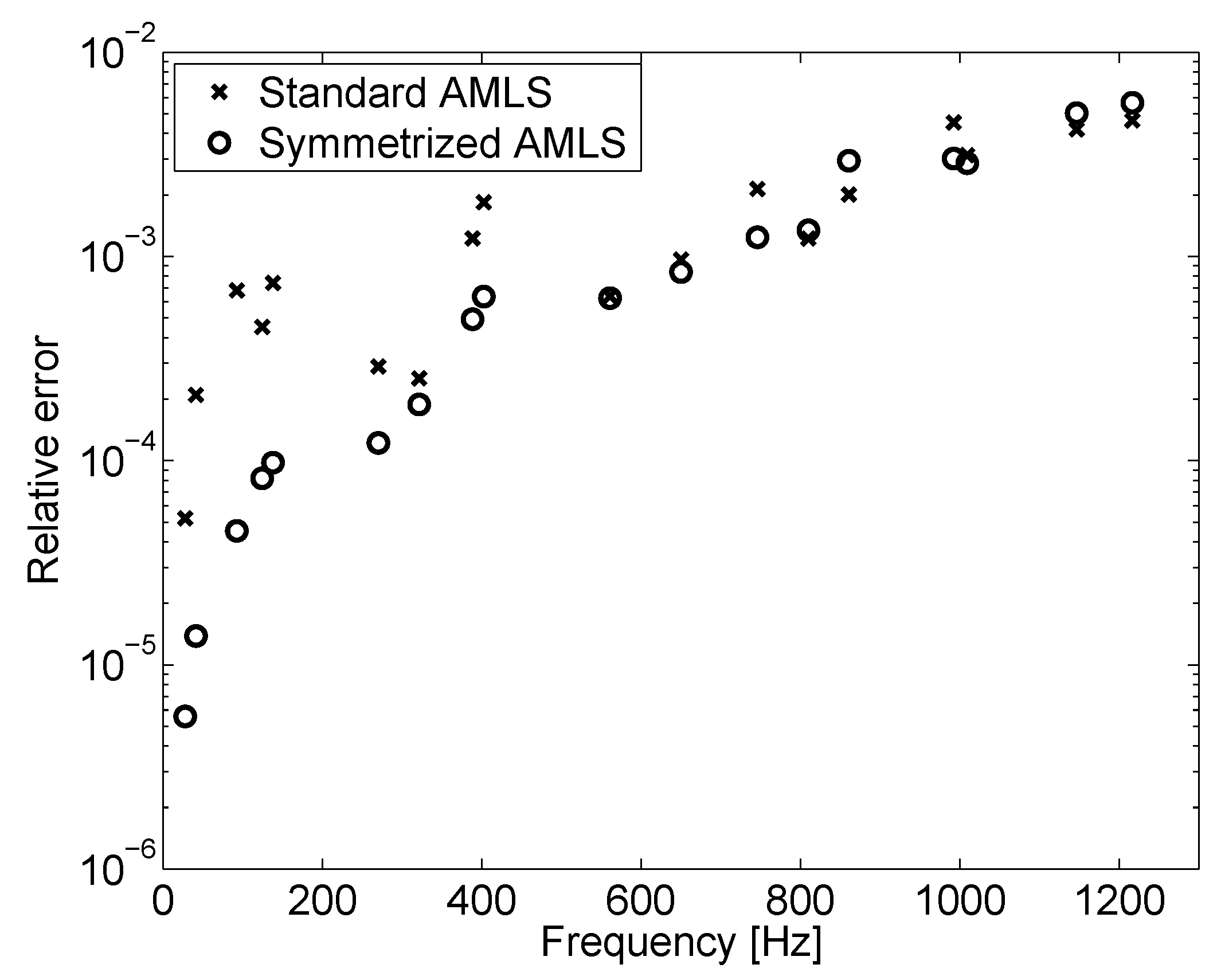
We applied the AMLS variant to the coupled fluid–solid problem and compared the eigenvalue approximations to those obtained from the standard procedure for the decoupled problem. In both cases, the algorithm was performed on 10 sub-structuring levels and 751 structures using a cut-off frequency corresponding to 10,000 Hz on each partitioning level. The relative errors are displayed in Figure 8.
The relative errors of the symmetrized AMLS method show the typical smooth behavior known from AMLS for self-adjoined eigenvalue problems. Eigenvalues with large accuracy improvements (e.g., Hz) turned out to belong to eigenforms with significant influence of the coupling. Eigenforms corresponding to larger eigenfrequencies were less influenced by the coupling, and in some cases, the eigenvalue approximations are slightly worse compared to the AMLS variant, neglecting the coupling effects in the reduction process. In all cases, the eigenvalue approximations were of larger magnitude than the exact eigenvalues.
7. Conclusions
For the non-self-adjoint elastoacoustic vibration problem describing the fluid by its pressure field and the structure by its displacement field, we have recapitulated variational characterizations of its eigenvalues generalizing Rayleigh’s principle, as well as minmax and maxmin characterizations. Discretizing the elastoacoustic problem with finite elements where the triangulation obeys the geometric partition into the fluid and the structure domain one obtains a non-symmetric matrix eigenvalue problem, which inherits the variational properties and the eigenvalues of which are upper bounds of the eigenvalues of the original problem. For the matrix eigenvalue problem, the Rayleigh functional iteration is cubically convergent as is the Rayleigh quotient iteration for linear symmetric problems and based on this structure-preserving iterative projection methods of the Jacobi–Davidson type and the nonlinear Arnoldi type can be defined. The automated multi-level sub-structuring method (AMLS) for linear eigenvalue problems in structural analysis can be generalized to the non-symmetric elastoacoustic problem, and an a priori error bound is proven, which usually overestimates the errors by orders of magnitude, but which cannot be improved without further assumptions. A numerical example demonstrates that the consideration of the coupling in the condensation process is indispensable if the coupling is strong.
Future research will be devoted to the improvement of the a priori bound for the automated multi-level sub-structuring method. The proof will be carefully checked in order to identify estimations, which can be reduced substantially taking advantage of information gained in the reduction process. Thus, we hope to arrive at an accurate a posteriori bound, which can serve for controlling the reduction process.
Conflicts of Interest
The author declares no conflict of interest.
References
- Belytschko, T. Fluid–structure interaction. Comput. Struct. 1980, 12, 459–469. [Google Scholar] [CrossRef]
- Craggs, A. The transient response of a coupled plate-acoustic system using plate and acoustic finite elements. J. Sound Vib. 1971, 15, 509–528. [Google Scholar] [CrossRef]
- Deü, J.-F.; Larbi, W.; Ohayon, R. Variational formulation of interior structural-acoustic vibration problem. In Computational Aspects of Structural Acoustics and Vibrations; Sandberg, G., Ohayon, R., Eds.; Springer: Wien, Austria, 2008; pp. 1–21. [Google Scholar]
- Ohayon, R. Reduced models for fluid–structure interaction problems. Int. J. Numer. Meth. Eng. 2004, 60, 139–152. [Google Scholar] [CrossRef]
- Petyt, M.; Lea, J.; Koopmann, G. A finite element method for determining the acoustic modes of irregular shaped cavities. J. Sound Vib. 1976, 45, 495–502. [Google Scholar] [CrossRef]
- Sandberg, G.; Wernberg, P.-A.; Davidson, P. Fundamentals of fluid–structure interaction. In Computational Aspects of Structural Acoustics and Vibrations; Sandberg, G., Ohayon, R., Eds.; Springer: Wien, Austria, 2008; pp. 23–101. [Google Scholar]
- Zienkiewicz, O.; Taylor, R. The Finite Element Method; McGraw-Hill: London, UK, 1991; Volume 2. [Google Scholar]
- Everstine, G. A symmetric potential formulation for fluid–structure interaction. J. Sound Vib. 1981, 79, 157–160. [Google Scholar] [CrossRef]
- Olson, L.; Bathe, K.-J. Analysis of fluid–structure interaction. A direct symmetric coupled formulation based on the fluid velocity potential. Comput. Struct. 1985, 21, 21–32. [Google Scholar] [CrossRef]
- Bathe, K.J.; Nitikipaiboon, C.; Wang, X. A mixed displacement-based finite element formulation for acoustic fluid–structure interaction. Comput. Struct. 1995, 56, 225–237. [Google Scholar] [CrossRef]
- Morand, H.; Ohayon, R. Substructure variational analysis of the vibrations of coupled fluid–structure systems. Finite element results. Int. J. Numer. Meth. Eng. 1979, 14, 741–755. [Google Scholar] [CrossRef]
- Sandberg, G.; Göranson, P. A symmetric finite element formulation for acoustic fluid–structure interaction analysis. J. Sound Vib. 1988, 123, 507–515. [Google Scholar] [CrossRef]
- Babuska, I.; Osborn, J. Eigenvalue problems. In Handbook of Numerical Analysis; Ciarlet, P., Lions, J., Eds.; North Holland: Amsterdam, The Netherlands, 1991; Volume II, pp. 641–923. [Google Scholar]
- Alonso, A.; Russo, A.-D.; Padra, C.; Rodriguez, R. A posteriori error estimates and a local refinement strategy for a finite element method to solve structural-acoustic vibration problems. Adv. Comput. Math. 2001, 15, 25–59. [Google Scholar] [CrossRef]
- Bermudez, A.; Gamallo, P.; Noguieras, N.; Rodriguez, R. Approximation of a structural acoustic vibration problem by hexahedral finite elements. IMA J. Numer. Anal. 2006, 26, 391–421. [Google Scholar] [CrossRef]
- Bermudez, A.; Rodriguez, R. Finite element computation of the vibration modes of a fluid–solid system. Comput. Meth. Appl. Mech. Eng. 1994, 119, 355–370. [Google Scholar] [CrossRef]
- Bermudez, A.; Rodriguez, R. Analysis of a finite element method for pressure/potential formulation of elastoacoustic spectral problems. Math. Comput. 2002, 71, 537–552. [Google Scholar] [CrossRef]
- Rodriguez, R.; Solomin, J. The order of convergence of eigenfrequencies in finite element approximations of fluid–structure interaction problems. Math. Comput. 1996, 65, 1463–1475. [Google Scholar] [CrossRef]
- Stammberger, M.; Voss, H. Variational characterization of eigenvalues of a non-symmetric eigenvalue problem governing elastoacoustic vibrations. Appl. Math. 2014, 59, 1–13. [Google Scholar] [CrossRef]
- Strutt, J.W. Some general theorems relating to vibrations. Proc. Lond. Math. Soc. 1873, 4, 357–368. [Google Scholar]
- Poincaré, H. Sur les equations aux dérivées partielles de la physique mathématique. Am. J. Math. 1890, 12, 211–294. [Google Scholar] [CrossRef]
- Courant, R. Über die Eigenwerte bei den Differentialgleichungen der mathematischen Physik. Math. Z. 1920, 7, 1–57. [Google Scholar] [CrossRef]
- Fischer, E. Über quadratische Formen mit reellen Koeffizienten. Monatshefte Math. 1905, 16, 234–249. [Google Scholar] [CrossRef]
- Weyl, H. Das asymptotische Verteilungsgesetz der Eigenwerte linearer partieller Differentialgleichungen (mit einer Anwendung auf die Theorie der Hohlraumstrahlung). Math. Ann. 1912, 71, 441–479. [Google Scholar] [CrossRef]
- Stammberger, M.; Voss, H. On an unsymmetric eigenvalue problem governing free vibrations of fluid–solid structures. Electr. Trans. Numer. Anal. 2010, 36, 113–125. [Google Scholar]
- Voss, H. A maxmin principle for nonlinear eigenvalue problems with application to a rational spectral problem in fluid–solid vibration. Appl. Math. 2003, 48, 607–622. [Google Scholar] [CrossRef]
- Voss, H. A minmax principle for nonlinear eigenproblems depending continuously on the eigenparameter. Numer. Linear Algebra Appl. 2009, 16, 899–913. [Google Scholar] [CrossRef]
- Hadeler, K.-P. Variationsprinzipien bei nichtlinearen Eigenwertaufgaben. Arch. Ration. Mech. Anal. 1968, 30, 297–307. [Google Scholar] [CrossRef]
- Voss, H. Variational principles for eigenvalues of nonlinear eigenproblems. In Numerical Mathematics and Advanced Applications—ENUMATH 2013; Abdulle, A., Deparis, S., Kressner, D., Nobile, F., Picasso, M., Eds.; Springer: Berlin, Germany, 2015; pp. 305–313. [Google Scholar]
- Voss, H. A Rational Spectral Problem in Fluid–Solid Vibration. Electr. Trans. Numer. Anal. 2003, 16, 94–106. [Google Scholar]
- Stammberger, M. On an Unsymmetric Eigenvalue Problem Governing Free Vibrations of Fluid–Solid Structures. Ph.D. Thesis, Hamburg University of Technology, Hamburg, Germany, 2010. [Google Scholar]
- ANSYS. Theory Reference for ANSYS and ANSYS Workbench; Release 11.0.; ANSYS, Inc.: Canonsburg, PA, USA, 2007. [Google Scholar]
- Ihlenburg, F. Sound in vibrating cabins: Physical effects, mathematical formulation, computational simulation with fem. In Computational Aspects of Structural Acoustics and Vibrations; Sandberg, G., Ohayon, R., Eds.; Springer: Wien, Austria, 2008; pp. 103–170. [Google Scholar]
- Kropp, A.; Heiserer, D. Efficient broadband vibro–acoustic analysis of passenger car bodies using an FE–based component mode synthesis approach. J. Comput. Acoust. 2003, 11, 139–157. [Google Scholar] [CrossRef]
- Bennighof, J.; Kaplan, M. Frequency window implementation of adaptive multi-level substructuring. J. Vib. Acoust. 1998, 120, 409–418. [Google Scholar] [CrossRef]
- Bennighof, J.; Lehoucq, R. An automated multilevel substructuring method for the eigenspace computation in linear elastodynamics. SIAM J. Sci. Comput. 2004, 25, 2084–2106. [Google Scholar] [CrossRef]
- Bai, Z.; Demmel, J.; Dongarra, J.; Ruhe, A.; van der Vorst, H. Templates for the Solution of Algebraic Eigenvalue Problems: A Practical Guide; SIAM: Philadelphia, PA, USA, 2000. [Google Scholar]
- Voss, H. An Arnoldi method for nonlinear eigenvalue problems. BIT Numer. Math. 2004, 44, 387–401. [Google Scholar] [CrossRef]
- Voss, H.; Stammberger, M. Structural-acoustic vibration problems in the presence of strong coupling. J. Press. Vessel Technol. 2013, 135, 011303. [Google Scholar] [CrossRef]
- Voss, H. A new justification of the Jacobi–Davidson method for large eigenproblems. Linear Algebra Appl. 2007, 424, 448–455. [Google Scholar] [CrossRef]
- Fokkema, D.; Sleijpen, G.; van der Vorst, H. Jacobi–Davidson style QR and QZ algorithms for the partial reduction of matrix pencils. SIAM J. Sci. Comput. 1998, 20, 94–125. [Google Scholar] [CrossRef]
- Saad, Y. Iterative Methods for Sparse Linear Systems, 2nd ed.; SIAM: Philadelphia, PA, USA, 2003. [Google Scholar]
- Sleijpen, G.; van der Vorst, H. A Jacobi–Davidson iteration method for linear eigenvalue problems. SIAM J. Matrix Anal. Appl. 1996, 17, 401–425. [Google Scholar] [CrossRef]
- Bennighof, J. Adaptive multi-level substructuring method for acoustic radiation and scattering from complex structures. In Computational Methods for Fluid/Structure Interaction; Kalinowski, A., Ed.; American Society of Mechanical Engineers: New York, NY, USA, 1993; Volume 178, pp. 25–38. [Google Scholar]
- Kaplan, M. Implementation of Automated Multilevel Substructuring for Frequency Response Analysis of Structures. Ph.D. Thesis, University of Texas at Austin, Austin, TX, USA, 2001. [Google Scholar]
- Elssel, K. Automated Multilevel Substructuring for Nonlinear Eigenvalue Problems. Ph.D. Thesis, Hamburg University of Technology, Hamburg, Germany, 2006. [Google Scholar]
- Gao, W.; Li, X.; Yang, C.; Bai, Z. An implementation and evaluation of the AMLS method for sparse eigenvalue problems. ACM Trans. Math. Softw. 2008, 34, 20. [Google Scholar] [CrossRef]
- Karypis, G.; Kumar, V. A Software Package for Partitioning Unstructured Graphs, Partitioning Meshes, and Computing Fill-Reducing Orderings of Sparse Matrices, Version 4.0; Technical Report; University of Minnesota: Minneapolis, MN, USA, 1998. [Google Scholar]
- Hendrickson, B.; Leland, R. The Chaco User’s Guide: Version 2.0; Technical Report SAND94-2692; Sandia National Laboratories: Albuquerque, NM, USA, 1994. [Google Scholar]
- Hurty, W. Dynamic analysis of structural systems using component modes. AIAA J. 1965, 3, 678–685. [Google Scholar] [CrossRef]
- Craig, R., Jr.; Bampton, M. Coupling of sub-structures for dynamic analysis. AIAA J. 1968, 6, 1313–1319. [Google Scholar]
- Elssel, K.; Voss, H. An a priori bound for automated multilevel substructuring. SIAM J. Matrix Anal. Appl. 2006, 28, 386–397. [Google Scholar] [CrossRef]
- Stammberger, M.; Voss, H. Automated multi-level sub-structuring for fluid–solid interaction problems. Numer. Linear Algebra Appl. 2011, 18, 411–427. [Google Scholar] [CrossRef]
Figure 1.
Geometry of the numerical example.
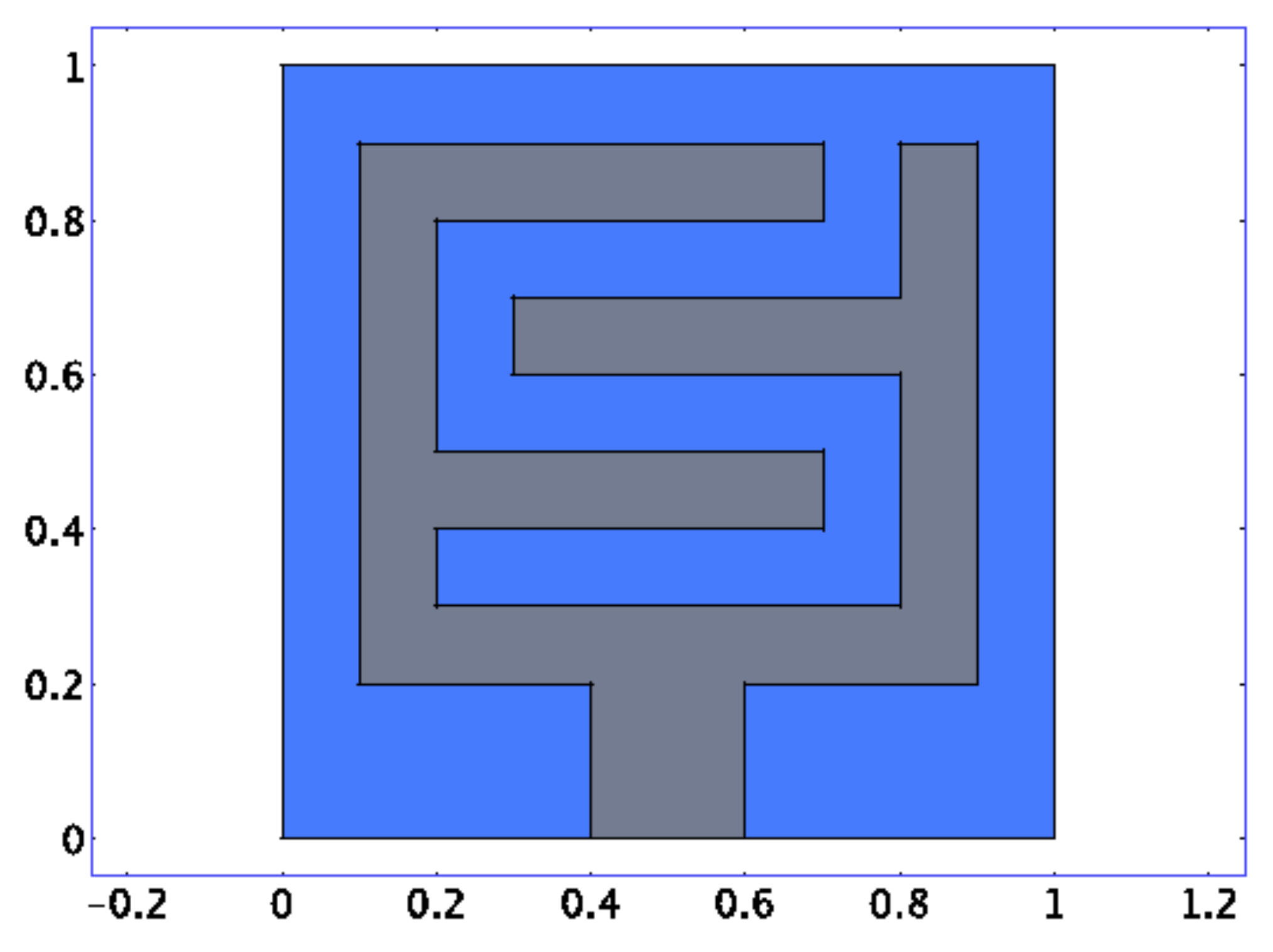
Figure 2.
Convergence history: nonlinear Arnoldi with block Cholesky preconditioner.
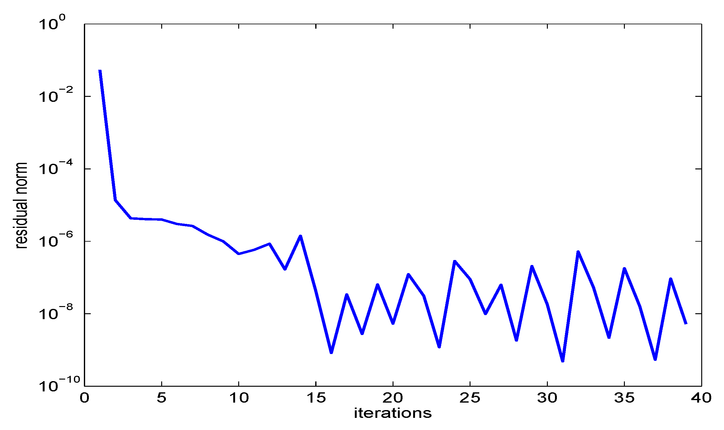
Figure 3.
Convergence history: Jacobi–Davidson with block Cholesky preconditioner.
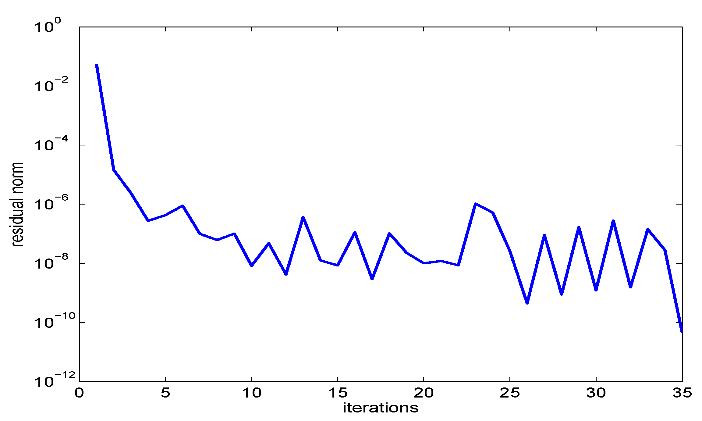
Figure 4.
Convergence history: nonlinear Arnoldi with incomplete LU preconditioner.
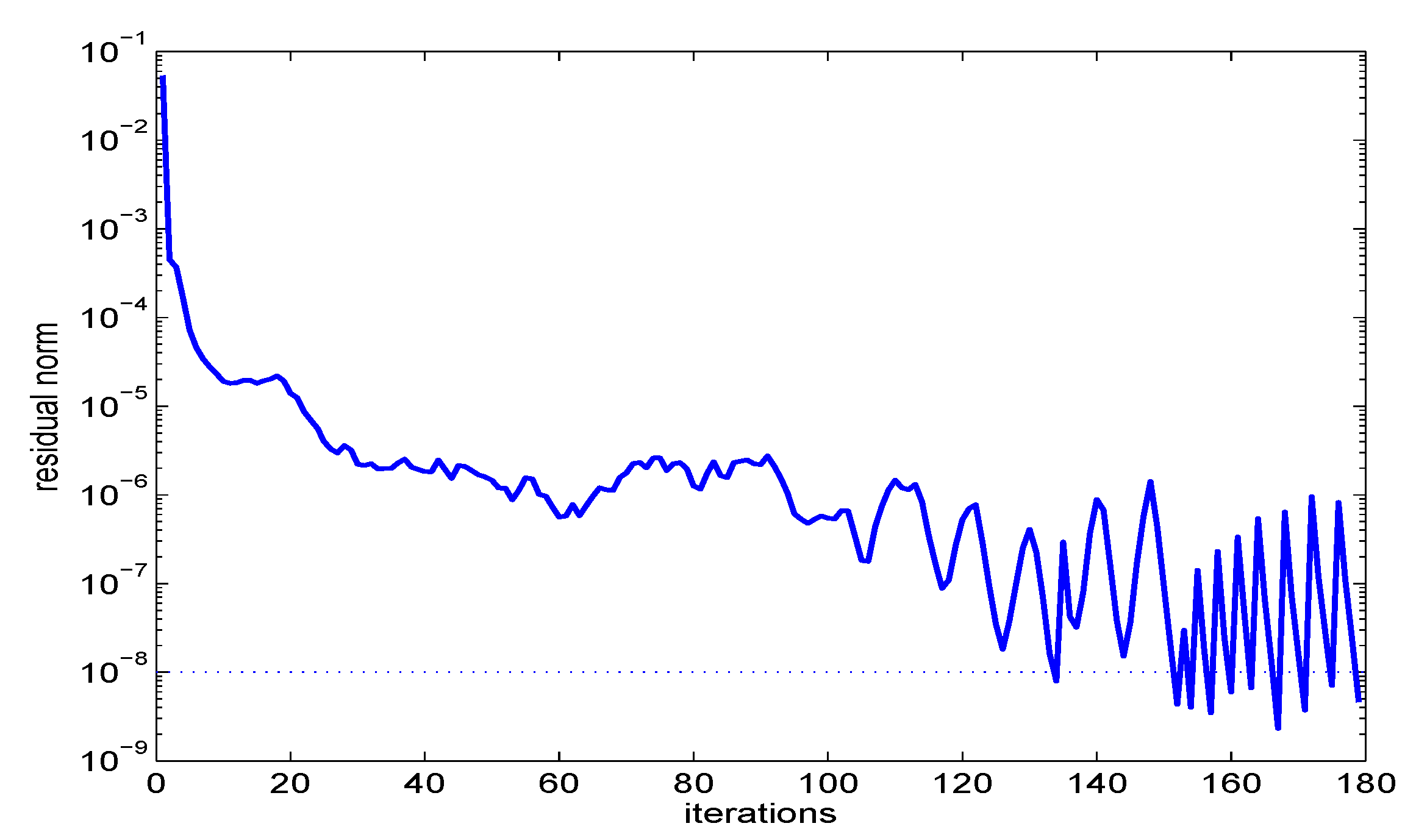
Figure 5.
Convergence history: Jacobi–Davidson with incomplete LU preconditioner.

Figure 6.
Arrowhead structure of the condensed mass matrix in automated multi-level sub-structuring (AMLS).
Figure 6.
Arrowhead structure of the condensed mass matrix in automated multi-level sub-structuring (AMLS).
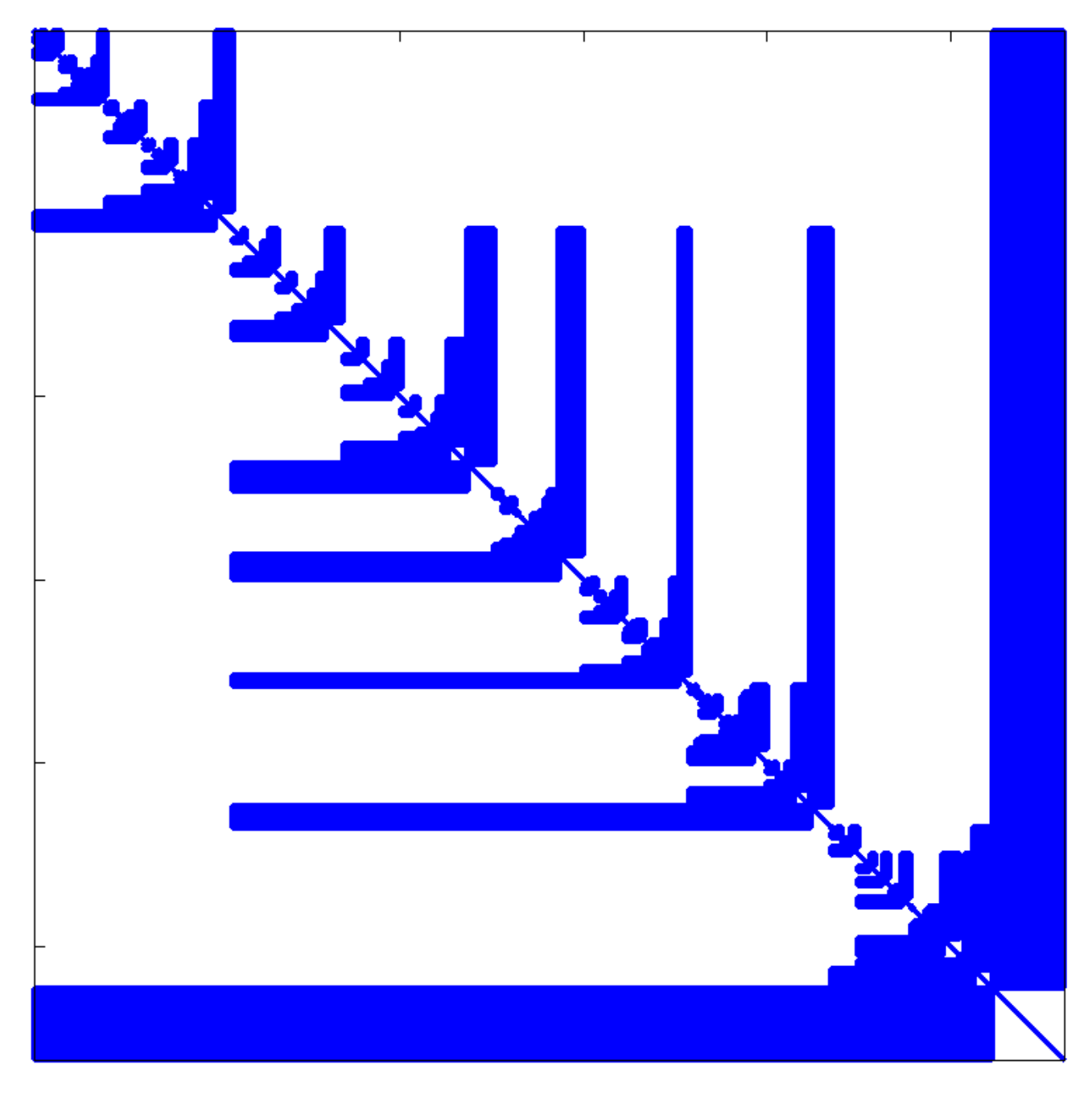
Figure 7.
A priori bound Equation (32) for Example 1.
Figure 7.
A priori bound Equation (32) for Example 1.
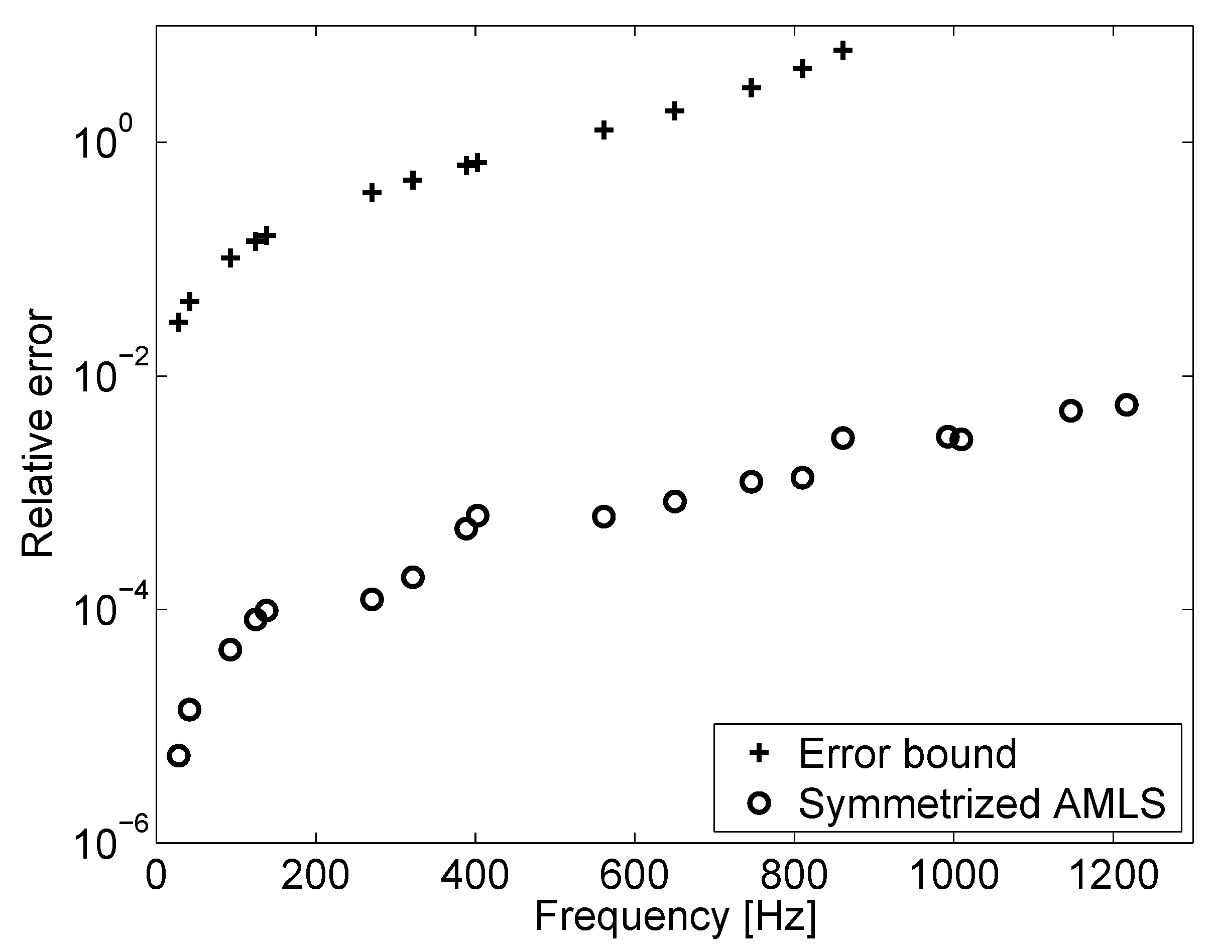
Figure 8.
Relative error of adapted AMLS for fluid–solid interaction problems and relative error of standard AMLS applied to fluid–solid interaction problems.
Figure 8.
Relative error of adapted AMLS for fluid–solid interaction problems and relative error of standard AMLS applied to fluid–solid interaction problems.


| Coupled | Steel | Air | Rel. Dev. | Rel. Err. Proj. |
|---|---|---|---|---|
| 0.00 | 0.00 | |||
| 41.25 | 41.32 | 0.16 | 2.5 × 10 | |
| 48.67 | 48.71 | 0.08 | 2.7 ×10 | |
| 56.96 | 56.90 | 0.11 | 2.2 ×10 | |
| 75.55 | 75.51 | 0.06 | 3.3 ×10 | |
| 93.18 | 93.19 | 0.01 | 1.0 ×10 | |
| 129.99 | 130.04 | 0.05 | 6.1 ×10 | |
| 150.94 | 151.03 | 0.06 | 3.5 ×10 | |
| 158.16 | 158.18 | 0.01 | 1.8 ×10 | |
| 186.64 | 186.66 | 0.12 | 4.2 ×10 |
| Coupled | Steel | Water | Proj. | Rel. Err. |
|---|---|---|---|---|
| 0.00 | 56.90 | 0.00 | 0.00 | |
| 28.01 | 75.51 | 178.63 | 28.33 | 1.2 |
| 41.54 | 151.03 | 210.64 | 43.01 | 3.5 |
| 92.73 | 186.66 | 402.93 | 101.98 | 10.0 |
| 124.70 | 225.54 | 133.60 | 7.1 | |
| 138.26 | 451.76 | 141.87 | 2.6 | |
| 270.40 | 472.45 | 285.18 | 5.5 | |
| 321.79 | 343.80 | 6.8 | ||
| 388.73 | 416.87 | 7.2 | ||
| 402.77 | 439.83 | 9.2 |
© 2016 by the author; licensee MDPI, Basel, Switzerland. This article is an open access article distributed under the terms and conditions of the Creative Commons Attribution (CC-BY) license (http://creativecommons.org/licenses/by/4.0/).
Share and Cite
MDPI and ACS Style
Voss, H. On a Non-Symmetric Eigenvalue Problem Governing Interior Structural–Acoustic Vibrations. Aerospace 2016, 3, 17. https://doi.org/10.3390/aerospace3020017
AMA Style
Voss H. On a Non-Symmetric Eigenvalue Problem Governing Interior Structural–Acoustic Vibrations. Aerospace. 2016; 3(2):17. https://doi.org/10.3390/aerospace3020017
Chicago/Turabian StyleVoss, Heinrich. 2016. "On a Non-Symmetric Eigenvalue Problem Governing Interior Structural–Acoustic Vibrations" Aerospace 3, no. 2: 17. https://doi.org/10.3390/aerospace3020017
Note that from the first issue of 2016, this journal uses article numbers instead of page numbers. See further details here.