Article

Vertical Wind Tunnel for Prediction of Rocket Flight Dynamics

1
Department of Electrical and Computer Engineering, University of Canterbury, Private Bag 4800, Christchurch 8140, New Zealand
2
Rocket Lab Ltd., 3A Airpark Drive, Auckland 2022, New Zealand
3
School of Engineering and Information and Communication Technology (ICT), University of Tasmania, Private Bag 65, Hobart 7001, Australia
4
Engineering and Architecture Department, Christchurch Polytechnic Institute of Technology (CPIT), P.O. Box 540, Christchurch Mail Centre, Christchurch 8140, New Zealand
5
Department of Mechanical Engineering, University of Canterbury, Private Bag 4800, Christchurch 8140, New Zealand
*
Author to whom correspondence should be addressed.
Aerospace 2016, 3(2), 10; https://doi.org/10.3390/aerospace3020010
Submission received: 1 February 2016 / Revised: 3 March 2016 / Accepted: 22 March 2016 / Published: 29 March 2016
(This article belongs to the Special Issue Innovations in Wind Tunnel Testing)

Abstract

:
A customized vertical wind tunnel has been built by the University of Canterbury Rocketry group (UC Rocketry). This wind tunnel has been critical for the success of UC Rocketry as it allows the optimization of avionics and control systems before flight. This paper outlines the construction of the wind tunnel and includes an analysis of flow quality including swirl. A minimal modelling methodology for roll dynamics is developed that can extrapolate wind tunnel behavior at low wind speeds to much higher velocities encountered during flight. The models were shown to capture the roll flight dynamics in two rocket launches with mean roll angle errors varying from 0.26° to 1.5° across the flight data. The identified model parameters showed consistent and predictable variations over both wind tunnel tests and flight, including canard–fin interaction behavior. These results demonstrate that the vertical wind tunnel is an important tool for the modelling and control of sounding rockets.

Graphical Abstract

1. Introduction

A customized vertical wind tunnel has been built by the University of Canterbury (UC) Rocketry Research group [1] to test advanced control systems for application on small sounding rockets at subsonic and supersonic speeds. The common approach to designing and analyzing supersonic rockets is to quantitatively identify aerodynamics in a supersonic wind tunnel. However, these types of wind tunnels have large power requirements and are thus very costly, and usually have much shorter run times around 0.1–0.2 s [2].
Another approach to subsonic and supersonic flow analysis is Computational Fluid Dynamics (CFD). For example, canard–fin interactions have been well studied and modelled with CFD using wind tunnel data with relatively good predictions for the smaller angle of attacks [3,4]. However, the available comparisons in the literature are usually for static movements of the canards, so it is not clear how well the CFD models predict transient response in flight. Only very limited comparisons between flight and wind tunnel data have been published and are typically old NASA technical notes (e.g., [5,6,7]). The results of [6] show a reasonable prediction of pitch flight dynamics in terms of the frequency and phase responses of the pitching velocity per unit canard-fin-deflection frequency, however no roll comparisons are given and CFD analysis is not performed. Hence, although CFD analysis is commonly used for predicting rocket response in a wind tunnel, it has not been fully validated in flight. For the case of hypersonic flow, no vehicle has been flown long enough to obtain the data needed to improve the model accuracy and hypersonic wind tunnels only provide very short durations. Thus, in general, although CFD are useful for gaining trends on the expected flight response, they are not sufficiently accurate to design robust control systems and hence, extensive flight testing is usually required.
In addition to CFD, there are a number of empirical approaches to modelling subsonic and supersonic rocket steady state aerodynamics. These methods are primarily based on NASA wind tunnel data and have been developed into engineering-level and intermediate-level aerodynamic prediction codes [7,8,9]. The models have also been extended to include canard interaction [10,11] but the experimental work is restricted to wind tunnels, so only considers steady state responses to fixed canard angles. Therefore, these methods are primarily for designing responsive canards in missiles and have not been used to understand actual rocket flight, where there are very fast movements and transient effects that often behave very differently to steady state response in a wind tunnel.
This paper develops models of rocket roll dynamics that are first identified in the wind tunnel at low speeds and then validated on actual rocket launches at much higher speeds. This type of validation is unique in the literature as most other approaches do not go any further than wind tunnel evaluation [10,11]. The UC rocketry modelling and control methodology is to use a combination of dynamic subsonic wind tunnel testing and sounding rocket launches, to test qualitatively methodologies that have the ability to account for new dynamics in real-time. In other words, the approach is to model the rocket response in the wind tunnel during a control actuation that will be implemented in a flight. In addition, the damping or lift coefficients are not needed to be precisely known before launch, as any uncertainty from the wind tunnel tests, can be accounted for “on-the-fly” during the rocket flight. This UC rocketry control methodology has been successfully validated on several subsonic launches including an unstable rocket. For more details and results see [1].
The vertical wind tunnel has been a critical component to the success of UC Rocketry. In particular, it is important for obtaining quantitative information on the first few seconds of flight and can be used to estimate a full subsonic flight response using minimal modelling and parameter identification [12]. In addition, the vertical test section allows a much simpler and more accurate way of testing roll dynamics since the rocket can be suspended from a string. In a standard horizontal wind tunnel there is extra friction since an additional moving surface, like a bearing is required, so roll response is less realistic. For pitch and yaw dynamics, a gimbal frame [13] is used to allow three° of freedom control. This gimbal frame set up is important for debugging the avionics control hardware and software before flight. To test the stability of a fully fueled rocket, two sets of strings are horizontally attached from one edge of the wind tunnel to the center of mass of the rocket, which allows movement in one axis. Hence this vertical wind tunnel has a number of unique features tailored for rocket flight analysis.
A typical closed-circuit subsonic horizontal wind tunnel has a motor powered fan which blows air around a looping tube [14]. The settling chamber usually contains a honeycomb flow straightener followed by several wire mesh screens to reduce turbulence [15]. Following the settling chamber, and just prior to the test section, is a contraction in the tube, which increases air speed. The test section is where the test article is placed and data is collected. A diffuser, which is a gradually diverging section of tube, is placed after the test section to decrease the velocity and thus decrease power requirements. Curved vanes guide air around corners [16]. The disadvantage of using a closed-circuit is that more space and materials are required to construct the back loop of the circuit. The curved vanes are complex features and an additional expense in the construction. Heat exchangers are often needed to keep the tunnel at the desired temperature, since the same air is being re-circulated through the circuit many times and may deviate significantly from the ambient air temperature [16].
A key part of the UC Rocketry wind tunnel design is the use of bendy plywood [17] due to its low cost, light weight and ease of constructing a circular cross section. Another advantage is that with a circular shape less material can be used to give the same cross-sectional area. That is, if the shape was changed to a square with side length equal to the circle’s diameter, the volume of space would be greater and manufacturing simpler, but the maximum displacement of the rocket that can be achieved in any direction, would still be the same as for the circle. Thus the extra power required in the fan to maintain a given flow velocity in the square configuration is effectively wasted. The vertical orientation also avoids the large floor and building space requirements needed for horizontal wind tunnels, and was assembled outdoors in a fenced enclosure further simplifying space allocation. A 15 kW fan was already in existence in the Department of Electrical and Computer Engineering at UC, so the wind tunnel was essentially built around this fan which was at the base and sitting on the ground.
This paper details some of the design and construction of the wind tunnel, methods for overcoming swirl induced from the fan, and presents a number of wind tunnel and flight results. A key finding is that the vertical wind tunnel can provide realistic roll predictions of rocket flights well beyond the wind speeds that can be generated by the current fan, and it provides an excellent test platform for modelling rocket behavior and validating parameter identification methods prior to flight. For example, similar canard–fin interaction roll dynamics observed and identified in the wind tunnel were also seen in the subsequent rocket flight. The results show that it is possible to create a low-cost wind tunnel with excellent flow characteristics, and thus provides a very valuable research tool for modelling and control of sounding rockets.

2. Methodology—Wind Tunnel

This section outlines the design and manufacture processes of the customized vertical wind tunnel used by UC Rocketry as shown in Figure 1.

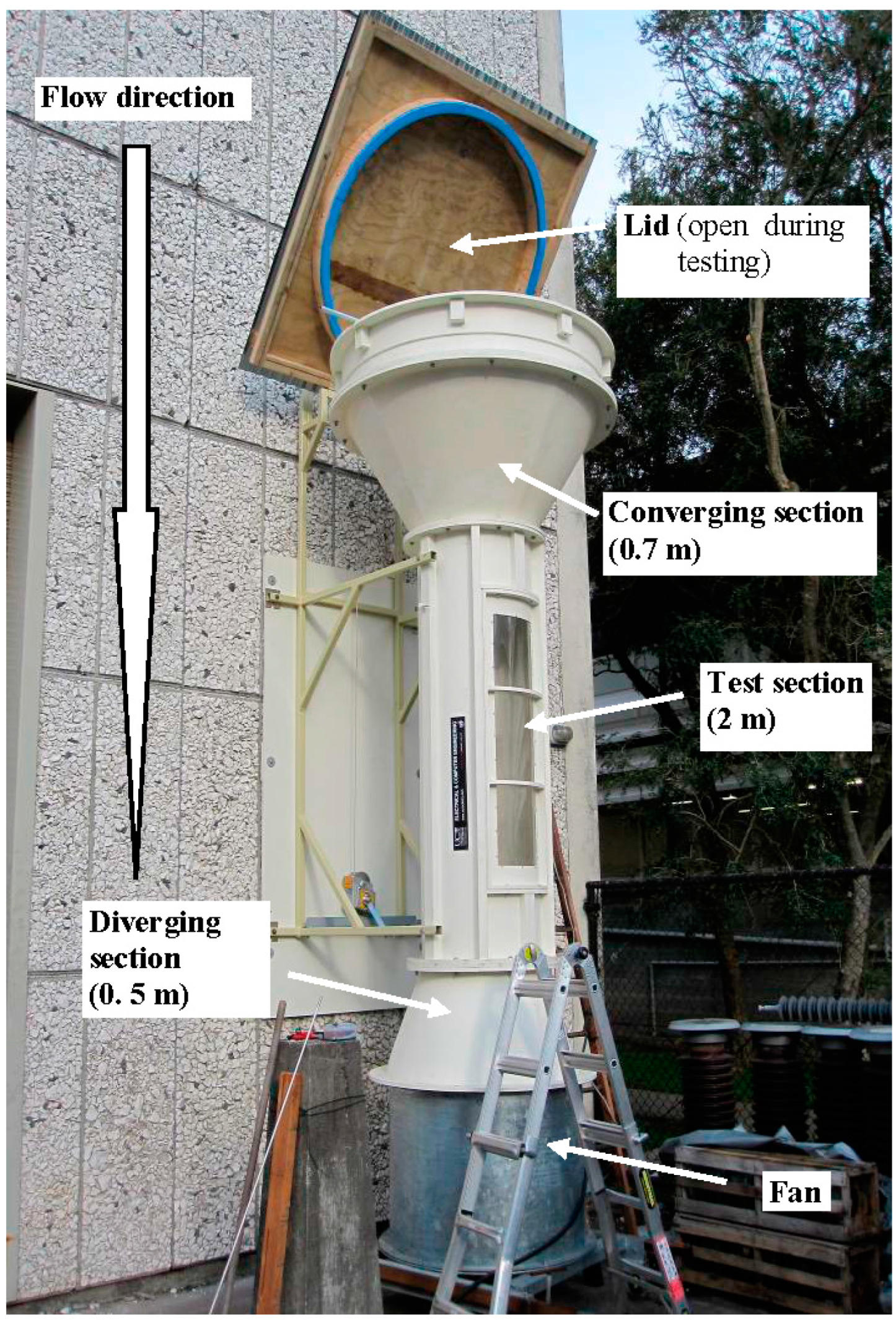
2.1. Concept and Design

To simplify the mounting of the rocket and to provide realistic roll response testing, the key design specification was to allow the mounting of the rocket vertically by suspending from the nose cone. Therefore a vertical suck-down wind tunnel was designed.
Due to the significant vertical height requirement, the structure was stored outside in a caged enclosure adjacent to the High Voltage Lab, which meant that it needed to be weather resistant. The wind tunnel was designed in individual sections with bolted joints between each section. This approach simplifies fabrication and assembly as the components could be added to or taken from the wind tunnel as required. To create a sufficient quality of flow in the wind tunnel, aluminium honeycomb was used as a flow conditioner. This flow straightener was critical, particularly since winds affect the flow.
Another important part of the design was utilizing an existing 1 m diameter, 15 kW fan and speed controller. Thus, the wind tunnel structure was effectively built around the fan. Since the test section was chosen to have a diameter of 0.6 m, wide angle diffusers were necessary to reduce the height of the wind tunnel. Bendy plywood was chosen for the structure as it was easy to form into the required shapes and significantly reduces manufacturing complexity and time, as compared to sheet-metal or fiberglass.
The overall rocket wind tunnel design consisted of five main components: the flow conditioner, reducer, test section, diffuser and fan. These components are summarized as follows:
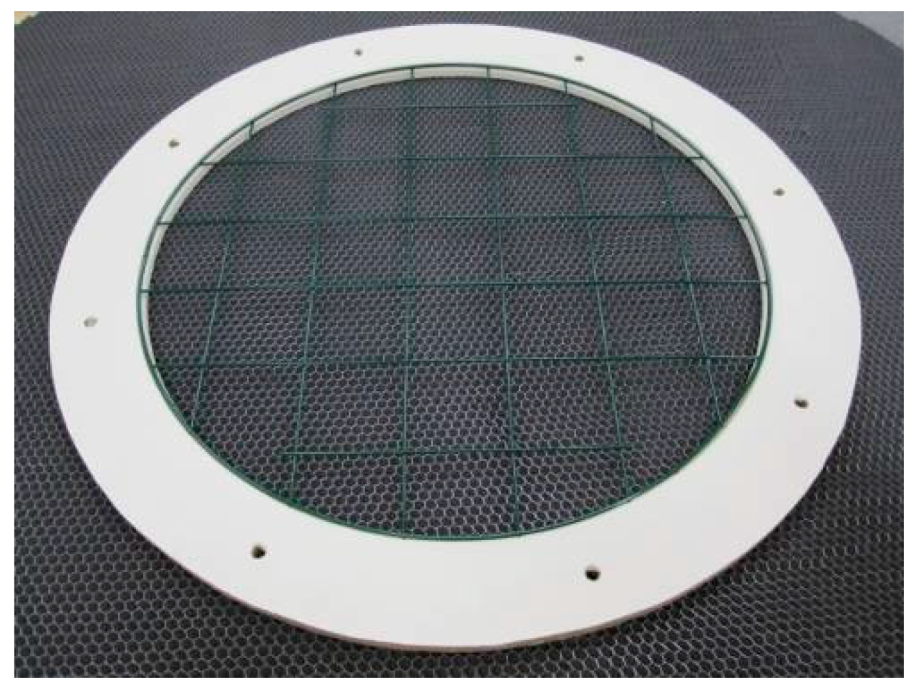
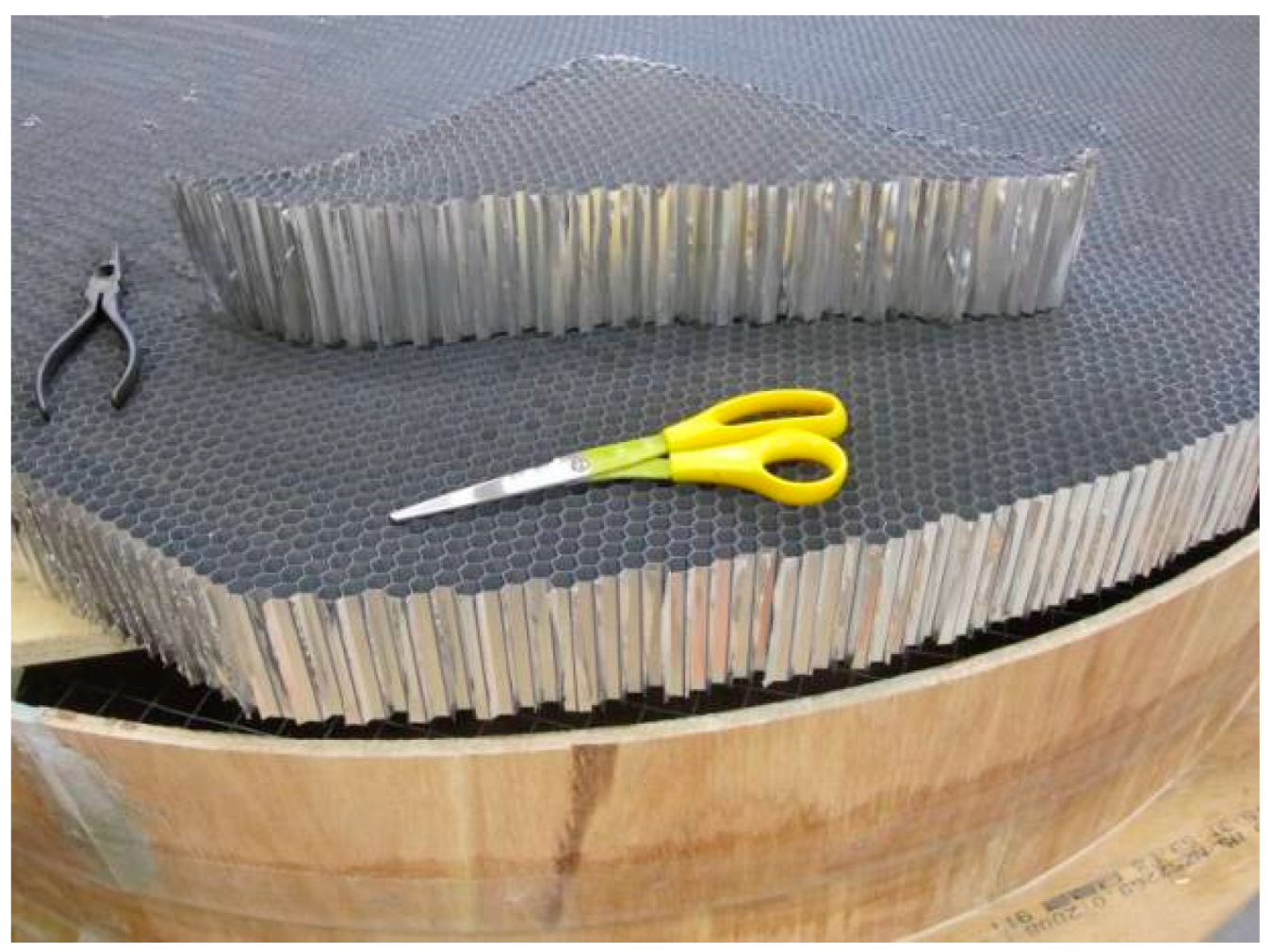
  • The flow conditioner was a cylindrical section at the inlet of the tunnel with an internal diameter of 1.4 m and a 9 mm wall thickness. The flow conditioner holds the honeycomb and a mesh screen.
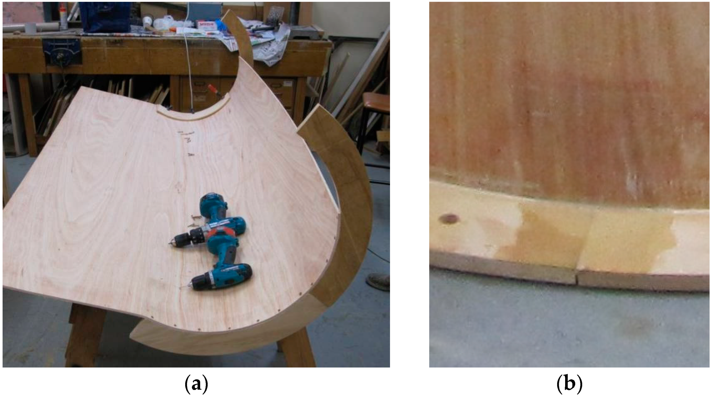
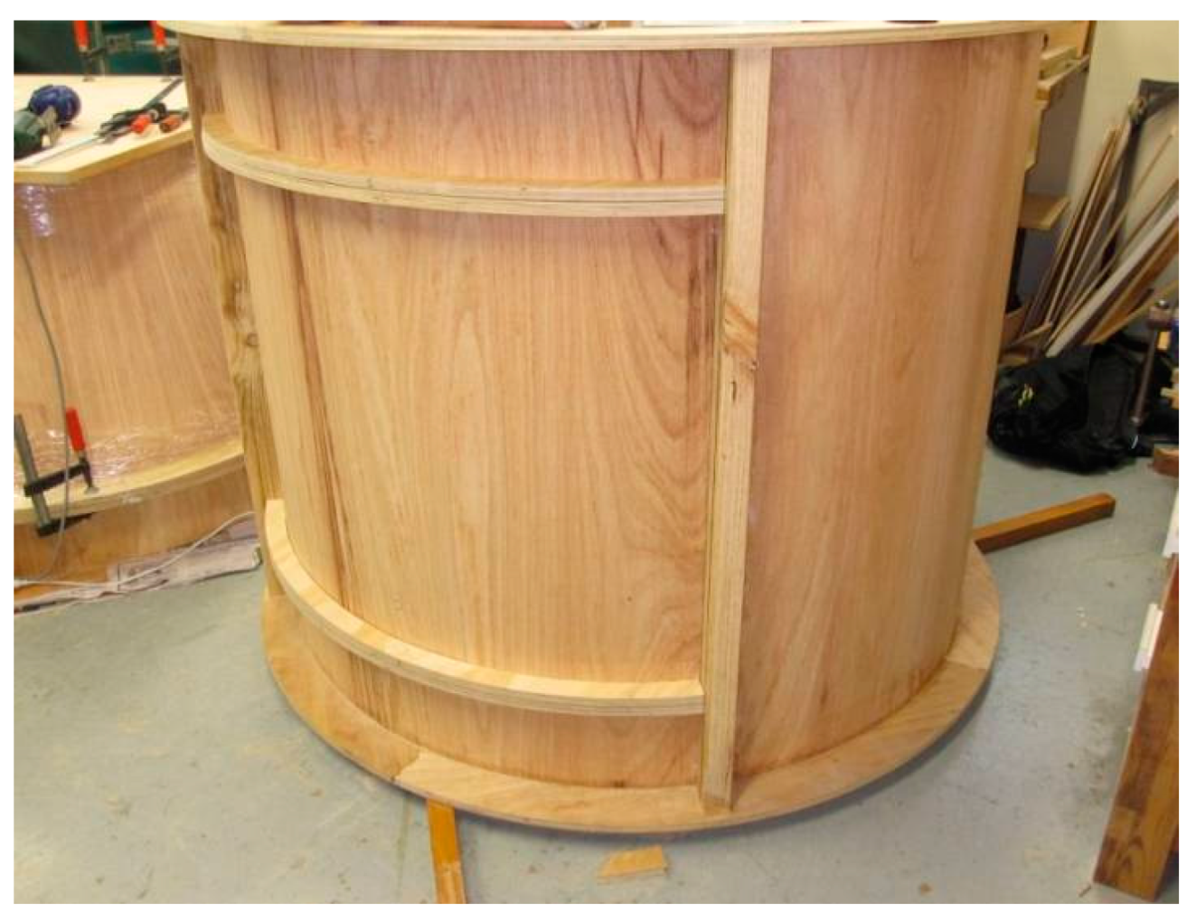
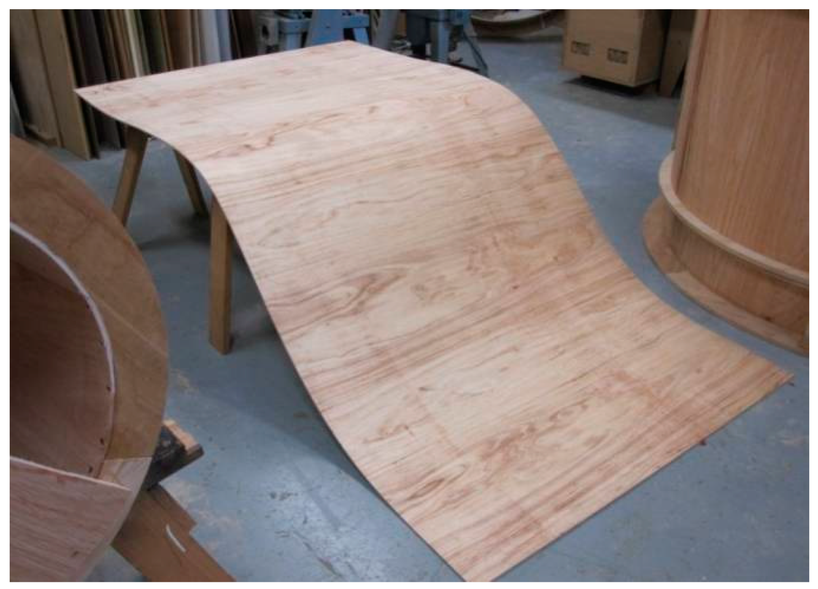
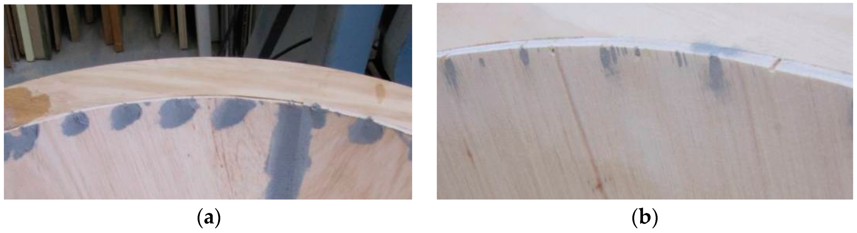
  • The reducer took the flow from the 1.4 m internal diameter flow conditioner to the 0.6 m internal diameter test section. This contraction before the test section can also reduce velocity fluctuations and form a more uniform flow. The reducer walls were fabricated from 6 mm bendy ply so that it would fit into the smaller internal diameter of the test section.
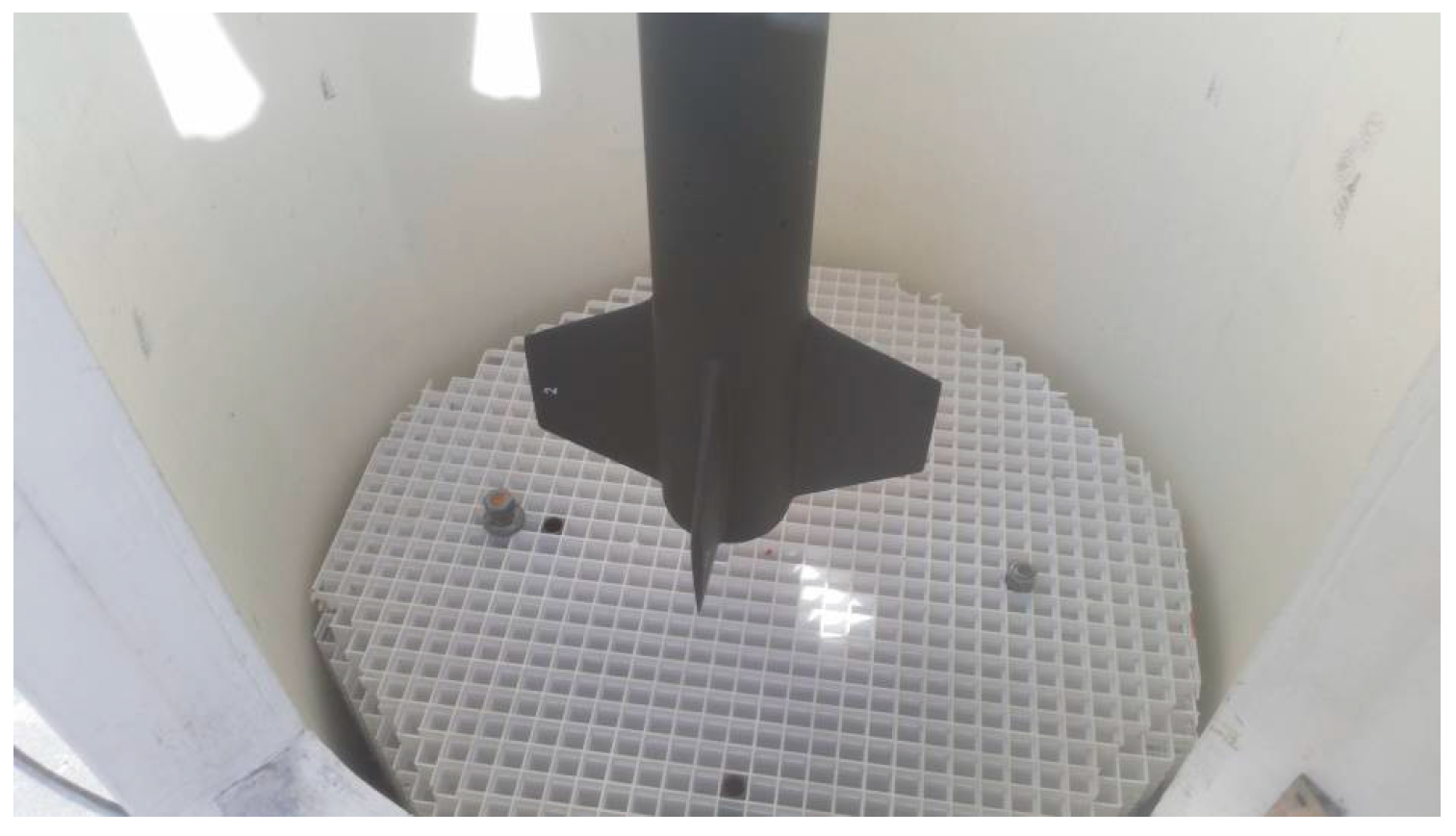
  • The test section was 2 m long, had an internal diameter of 0.6 m and was formed with 6 mm bendy ply. Due to the length and thin walls of the test section a 77 × 38 mm length of pine was run down each side. The door for the test section was then framed using 75 × 38 mm pine and 17 mm plywood. The frame was then removed and the door cut from the test section. At the bottom of the test section, a metal grille recessed into a plywood ring was placed to protect the fan.
  • The diffuser transitioned the flow from the 0.6 m internal diameter test section to the 1 m internal diameter fan housing. The diffuser was also made from 6 mm bendy ply.
  • The fan was 1 m diameter and had up to 15 kW available in power. The blade angle was at 23° so was left unchanged. The fan was on wheels, and could be adjusted to meet flush with the diffuser.
In addition, the wind tunnel was secured to the wall of the High Voltage (HV) lab by a permanent scaffold and a winch was used to open a lid on the wind tunnel during operation and closed after testing to ensure no rain came into the wind tunnel and fan.

2.2. Construction

2.2.1. General Methods

Bendy ply was used for the outer skin of the wind tunnel. Bendy ply is plywood with the two outer lamination grains aligned, and forming most of the thickness of the sheet. A thin central lamination bonded the two outer laminations together with the grain running perpendicular to the outer laminations. This property allows the plywood to be bent down to tight radii without the need for steam/heat, see Figure 2.
The rest of the tunnel structure was constructed from standard 17 mm plywood and 75 × 38 mm pine. The 17 mm plywood was used to form the flanges on the ends of each section. To reduce the amount of material wastage, each flange was made up from four quarter flanges. The parts were cut using a jigsaw. The sections of the wind tunnel were fabricated by forming individual outer skin pieces to the flanges, and securing with wood screws, as shown in Figure 3a. Once a complete section had been secured, the screws were backed off, epoxy resin with West Systems 403 modifier was worked into the gap, and the screws were again tightened. The flange joints were then reinforced with 200 g woven fiberglass cloth, see Figure 3b. The 75 × 38 mm pine was used to add strength to the openings in the tunnel and provide mounting points for fixtures, see Figure 4.
The internal surface of the tunnel was not perfectly smooth due to the outer skin joints, screw-heads, excess glue and manufacturing imperfections on the inner plywood face. Therefore, all internal surfaces and flange faces were sanded smooth. It was also necessary to fill voids on the inner side of the skin; both along the seams and behind the screw heads. Poly-filler was applied to these areas and sanded back, so that the flow in the tunnel would not be disrupted, as shown in Figure 5.

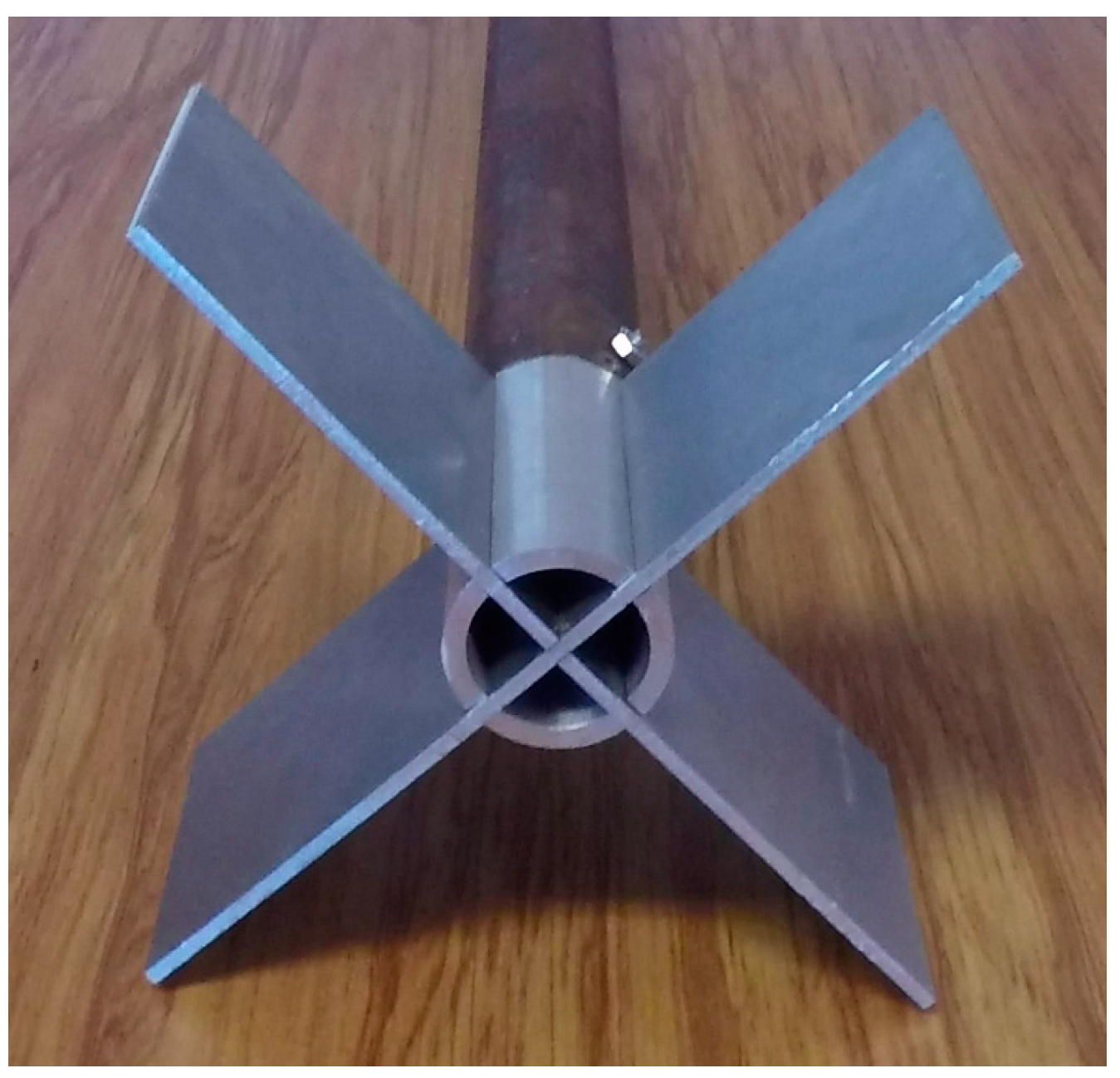
2.2.2. Flow Conditioner and Fan Grille

The flow conditioner was constructed similarly to the rest of the tunnel but required some additional features. To support the honey comb, a 9 mm ledge was built for it to rest upon. In addition, a galvanized wire mesh was put across the flow conditioner. The square sheet of honeycomb was cut to fit the circular flow conditioner, see Figure 6.
To prevent damage to the fan due to falling objects, a simple grille was fabricated. A plywood ring was cut with an internal diameter matching the internal diameter of the test section, and outside diameter matching the outer diameter of the flanges. A recess was cut along the inside edge of the flange using a router to form a ledge for the grille to rest on, as shown in Figure 7.

3. Methodology—Rocket Systems and Modelling

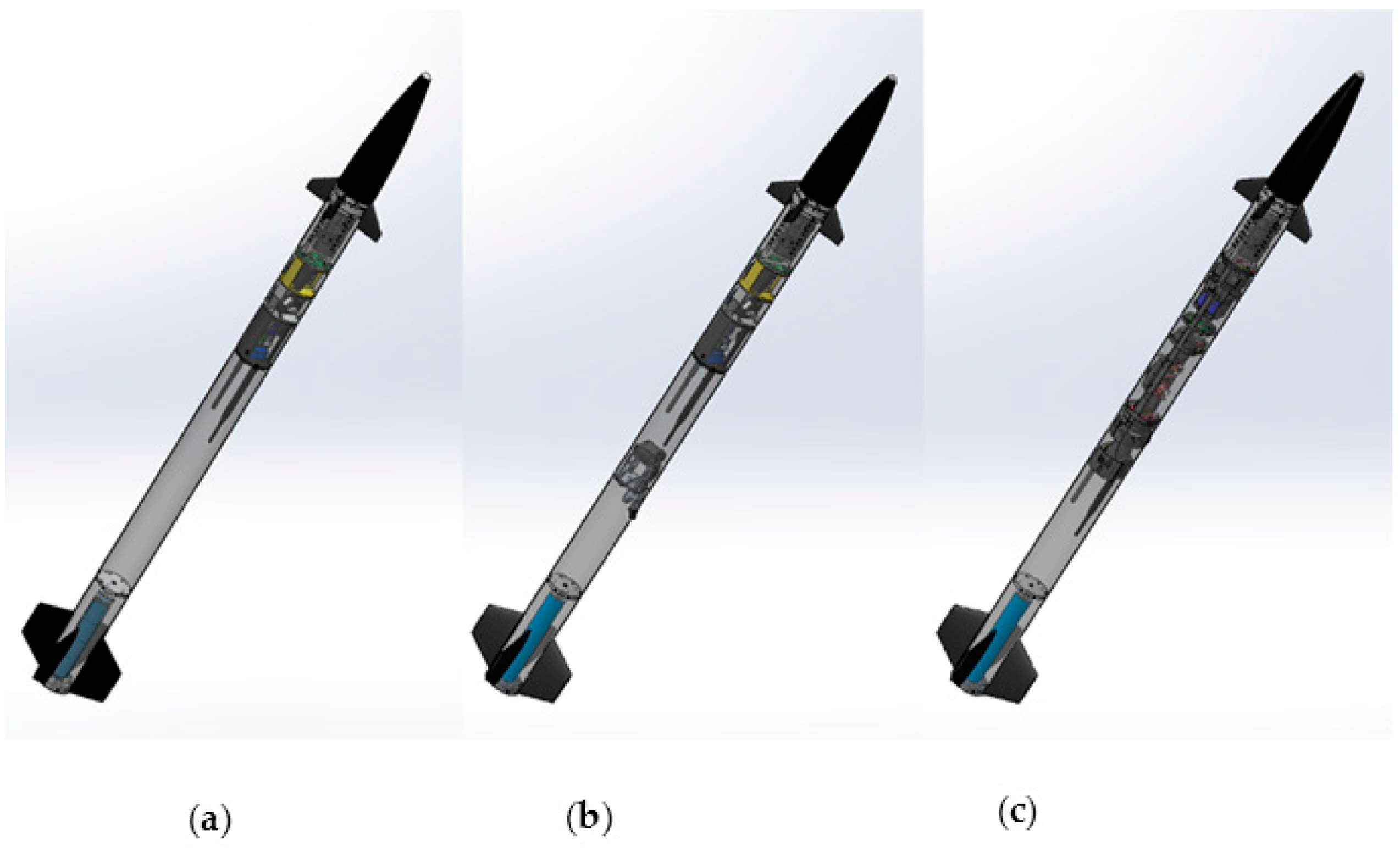
3.1. Improvements to Airframe and Avionics Stack

Since the launch of Smokey at the end of 2014 [12], there have been a number of improvements implemented to the rocket systems. These improvements can be seen in Figure 8, which shows the three launch configurations of the Smokey and Tasha III airframes. The Smokey and Tasha III airframe designs are aerodynamically equivalent. Both designs have identical canard, fin, tube length, tube diameter and nose cone geometry. The main difference between the two airframes was the manufacturing process for attaching the back fins.
Smokey used Acrylonitrile butadiene styrene (ABS) 3D printed fins and canards. The strength of these parts were appropriate for subsonic flight; however, they can be damaged on landing resulting in more time spent repairing the airframe. To overcome this problem, Tasha III also used 3D printed fins, but they were laminated to the airframe with fiberglass. Two of the Tasha III’s 3D printed canards were damaged after its first flight, so on its second flight we used our supersonic capable stack, which has fiberglass canards.
Cameras were placed in Tasha III allowing the recording of flights to provide an insight on how the on-board avionics were performing. Some holes were cut in the airframe, with one of the cameras placed out one side of the airframe by 10 mm. Smokey did not use an on-board camera, so it had no camera holes.
UC Rocketry’s supersonic launches require a device to report where the rocket lands. Both Tasha III flights included the Spot Tracker to test its capability to report landing locations. The Spot Tracker and cameras are the main reason the Tasha III vehicle was heavier than Smokey. The second Tasha III launch was heavier than the first Tasha III launch, because the avionics were exchanged to the more robust supersonic capable avionics.
Each launch of the Smokey and Tasha III airframes had different properties. Between each launch, changes were made to the internal avionics which affects the mass of the vehicle. Changes in mass affect the torques and airspeeds experienced during flight. Table 1 summarizes the key differences between the vehicles for each launch.

3.2. Testing Rocket Stability

A major advantage of the vertical wind tunnel is that it is a straightforward way to test rocket stability before flight. UC Rocketry has developed the following procedure for testing stability:
  • Assemble the rocket with a dummy mass motor.
  • Measure the center of mass by balancing the rocket on a beam less than 20 mm wide. Mark the center of mass.
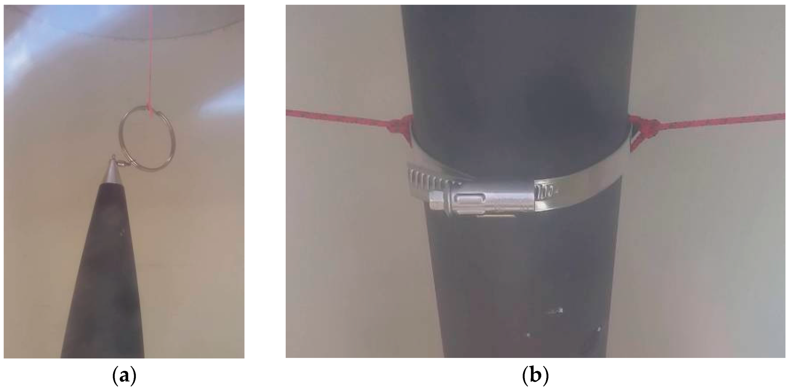
  • Fix a pipe clamp, with string tied securely to both ends of the pipe clamp to the rocket, at the measured center of mass.
  • Feed the string from both sides of the clamp through the two 4 mm holes on the sides of the wind tunnel. Tie the string around the back of the wind tunnel, and tension the ropes to lift the center of mass of the rocket as close as possible to the holes in the side of the wind tunnel.
  • Attach the nose tip of the rocket to the vertical string. The purpose of this string is to prevent an unstable rocket from damaging the walls, or prevent the rocket from falling should the clamps slip. The vertical string should be taut only when the nose of the rocket is close to the wind tunnel walls.
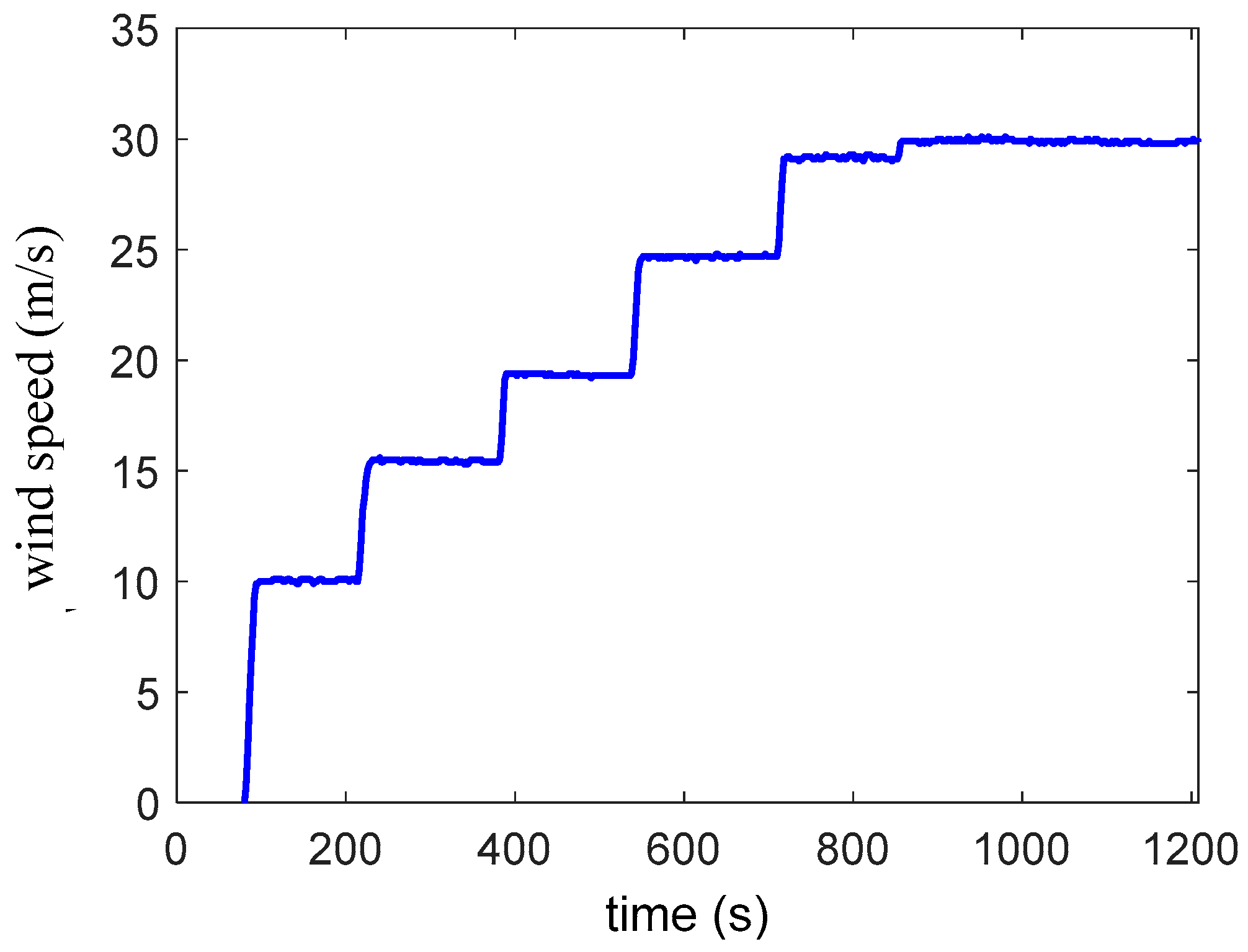
  • Start the wind tunnel, and check the rocket straightens at 15, 20 and 30 m/s.
Figure 9 gives a picture of a stability test set up.
Since these tests were for roll control only, the exact margin of stability in terms of the number of calibres, was not determined. The main aim of the test in Figure 9, was to prove general stability so that it would be safe to launch. An experimental determination of the center of pressure using this method will be investigated in future work for pitch and yaw modelling.

3.3. Rocket Roll Dynamics Modelling

In both launches and all wind tunnel tests in this paper, only roll dynamics were investigated. This section outlines the modelling and parameter identification techniques used to understand and predict the rocket roll dynamics during flight.

3.3.1. Minimal Model

The roll model is extended from a previously used model [12] which includes the effect of velocity on the damping and normal forces in the roll axis. Ignoring the yaw term in Equation (6) of [13] and lumping the parameter d into the coefficients of the roll fin angle and damping yields:
I p p ˙ = 1 2 ρ v 2 A [ β u f i n ( t ) α v p ]
where the definition of the parameters is given in the Notation. Expanding out Equation (1), and including the effects of disturbance and defining the roll angle gives the differential equation model:
I p p ˙ = 1 2 ρ v A α p + 1 2 ρ v 2 A β ( u f i n ( t ) + u d i s t ( t ) )
ϕ ˙ = p
where u d i s t ( t ) u d i s t ( t ) lumps the effects of fin canard interaction, thrust offsets that may impart a roll and atmospheric effects into a single time-varying parameter. It is shown in the results section that when there are sudden fin movements, it’s critical to allow fast changes in the disturbance at these points to provide a good match to the data. To model these effects, the disturbance is written in the form:
u d i s t ( t ) = k = 1 N Y k Φ k
Y k = u d , k 1 + ( u d , k u d , k 1 ) ( T k T k 1 ) ( t T k 1 )
Φ k = H ( t T k 1 ) H ( t T k )
where
H ( t ) heaviside function ,       T 0 , , T N user defined time points
u d , 0 , , u d , N unknown constants identified from data

3.3.2. Parameter Identification

To ensure the optimum possible model is obtained with good numerical parameter identifiability, a grid search is applied to the main parameters excluding the disturbance, which is identified using non-linear regression. This method was applied for both an open-loop model, where u f i n ( t ) is measured directly by encoders on the rocket and a closed-loop model where u f i n ( t ) is defined from a standard proportional derivative controller plus the addition of a pre-defined input. Mathematically these models are defined:
Open-loop :       u f i n ( t ) = u f i n , O L ( t ) fin movement measured from encoder
Closed-loop :       u f i n ( t ) = u f i n , C L ( t ) = k p ( R ( t ) ϕ ( t ) ) + k d ( R ( t ) p ( t ) ) + u i n p u t ( t )
where
k p proportional gain ,         k d derivative gain
R ( t ) = ( R 0 R 1 ) H ( sin ( 2 π f 0 t ) ) + R 1
The reference function R ( t ) in Equation (12) is an alternating square wave of frequency f 0 (Hz) between the values of R 0 and R 1 . This function allows multiple step responses to be analyzed from wind tunnel tests and rocket flights. The function u i n p u t ( t ) is set to 0 for the wind tunnel tests and the first flight, but is defined as a chirp function with varying amplitudes for the second flight to increase flight dynamics for a rigorous test of the model.
The optimization is set up by first fixing the damping α and torque constant β . Two objective functions are defined:
F α , β O L ( U d ) = [ ϕ d a t a ( t 0 ) ϕ O L ( t 0 ) , , ϕ d a t a ( t e n d ) ϕ O L ( t e n d ) ]
F α , β C L ( U d ) = [ ϕ d a t a ( t 0 ) ϕ C L ( t 0 ) , , ϕ d a t a ( t e n d ) ϕ C L ( t e n d ) ]
U d = [ u d , 0 , , u d , N ] T
where
ϕ d a t a ( t ) measured roll angle ,       t 0 , , t e n d     data time points
ϕ O L ( t ) roll angle solution to Equations ( 2 ) ( 9 )  for given  α , β  and  U d
ϕ C L ( t ) roll angle solution to Equations ( 2 ) ( 8 ) , ( 10 ) ( 12 ) ,  for given    α , β  and  U d
A range of values of α and β are then selected:
α = { α m i n + k Δ α , k = 0 , , N α } , β = { β m i n + k Δ β , k = 0 , , N β }
For each α and β from the ranges in Equation (19), the open-loop and closed-loop identified disturbance values are defined:
U ^ d O L =  non-linear least squares solution to Equation  ( 13 )
U ^ d C L =  non-linear least squares solution to Equation  ( 14 )
The final model parameters that best fit the data are then defined:
X O L = [ α O L , β O L , U ^ d O L ]    :    F α O L , β O L O L ( U ^ d O L )     = min { α α , β β } ( mean | F α , β O L ( U ^ d O L ) | )
X C L = [ α C L , β C L , U ^ d C L ]    :    F α C L , β C L C L ( U ^ d C L )     = min { α α , β β } ( mean | F α , β C L ( U ^ d C L ) | )
Equations (22) and (23) represent a grid search over all the values in Equation (19), where for each pair of α and β a non-linear regression is performed to determine the corresponding disturbance values. This non-linear regression uses the command “lsqnonlin” in Matlab.

4. Results and Discussion

4.1. Wind Tunnel Flow Quality

Measurements from a hot wire anemometer placed at various positions from the boundary showed that there are negligible boundary effects greater than 200 mm from the wall, with less than 5% reduction in wind speed at 100 mm from the wall. Since the diameter of the sounding rockets in this research are 80 mm with a 60 mm canard and fin radial distance, the outermost point of the rocket is 160 mm from the wall. Hence, the volume of the test section used in this research, has close to uniform flow. Most importantly, the results from the prediction of rocket flight roll response from wind tunnel derived parameters presented in the sections below, demonstrate that the test section has adequate flow quality for this research.

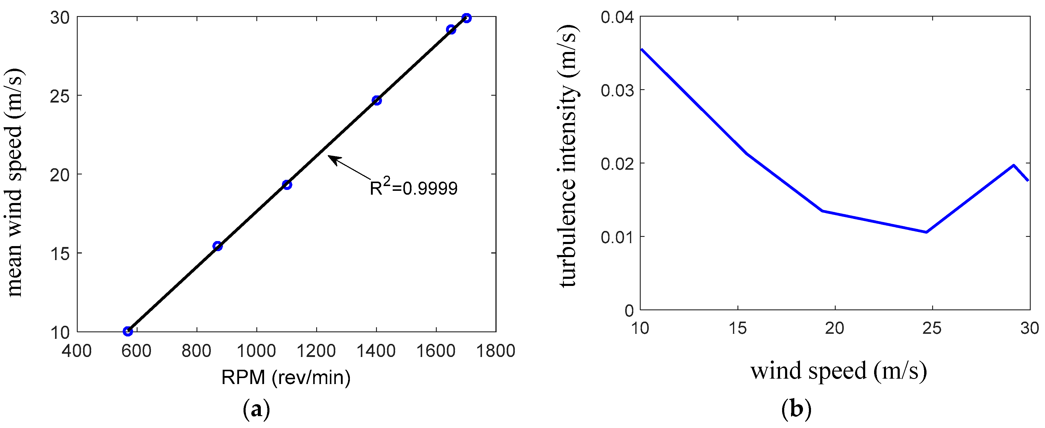
4.1.1. Turbulence Intensity
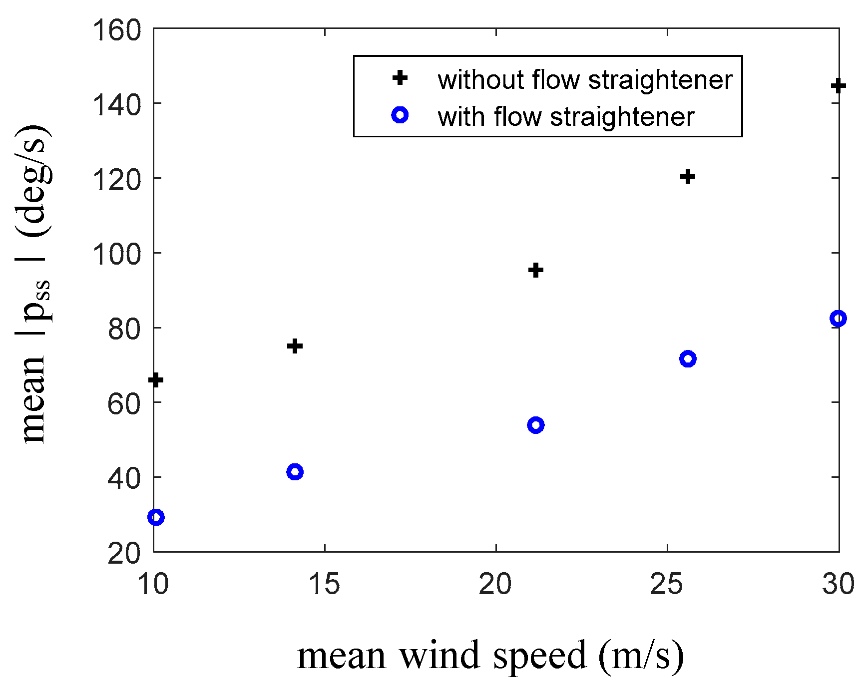
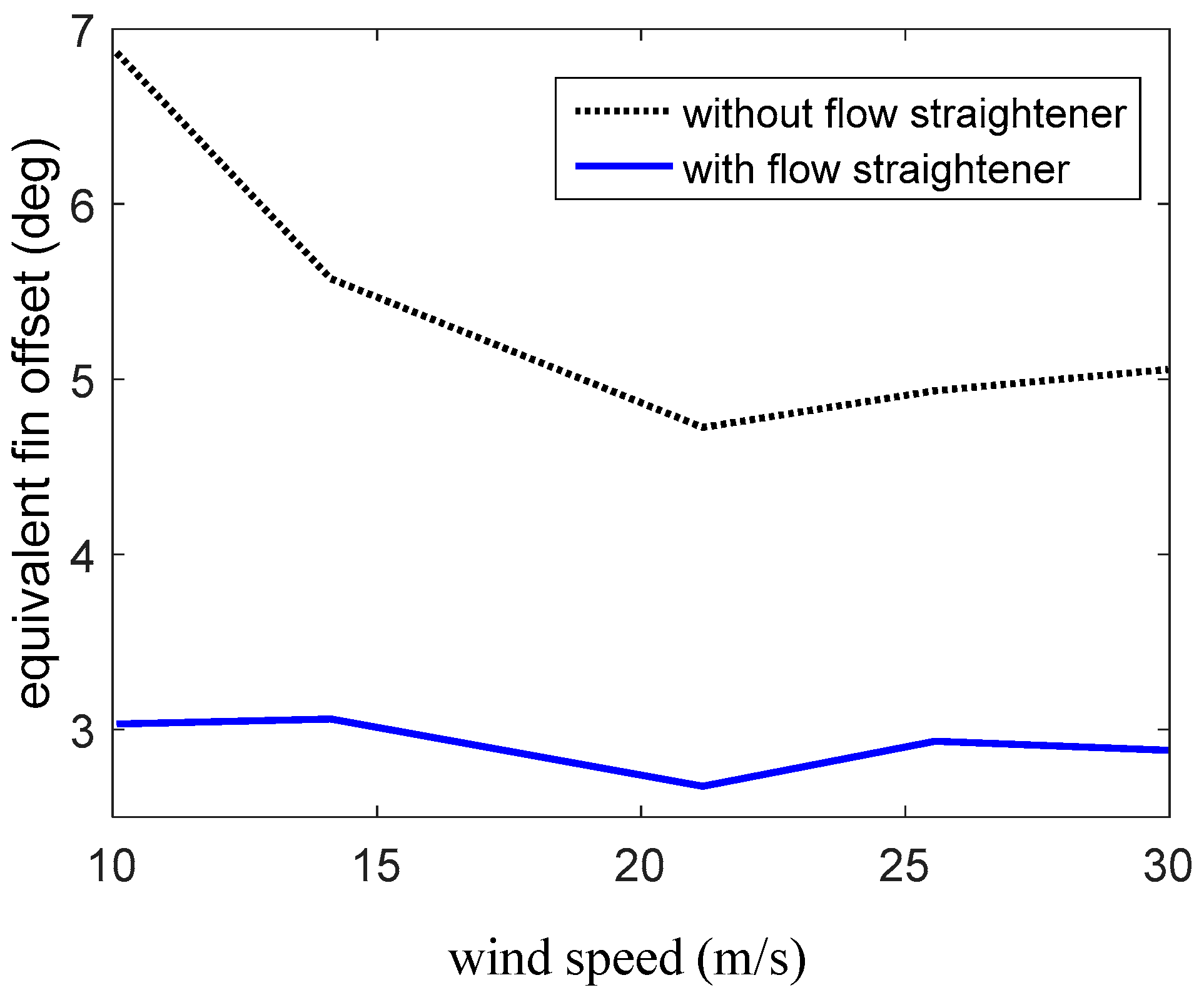
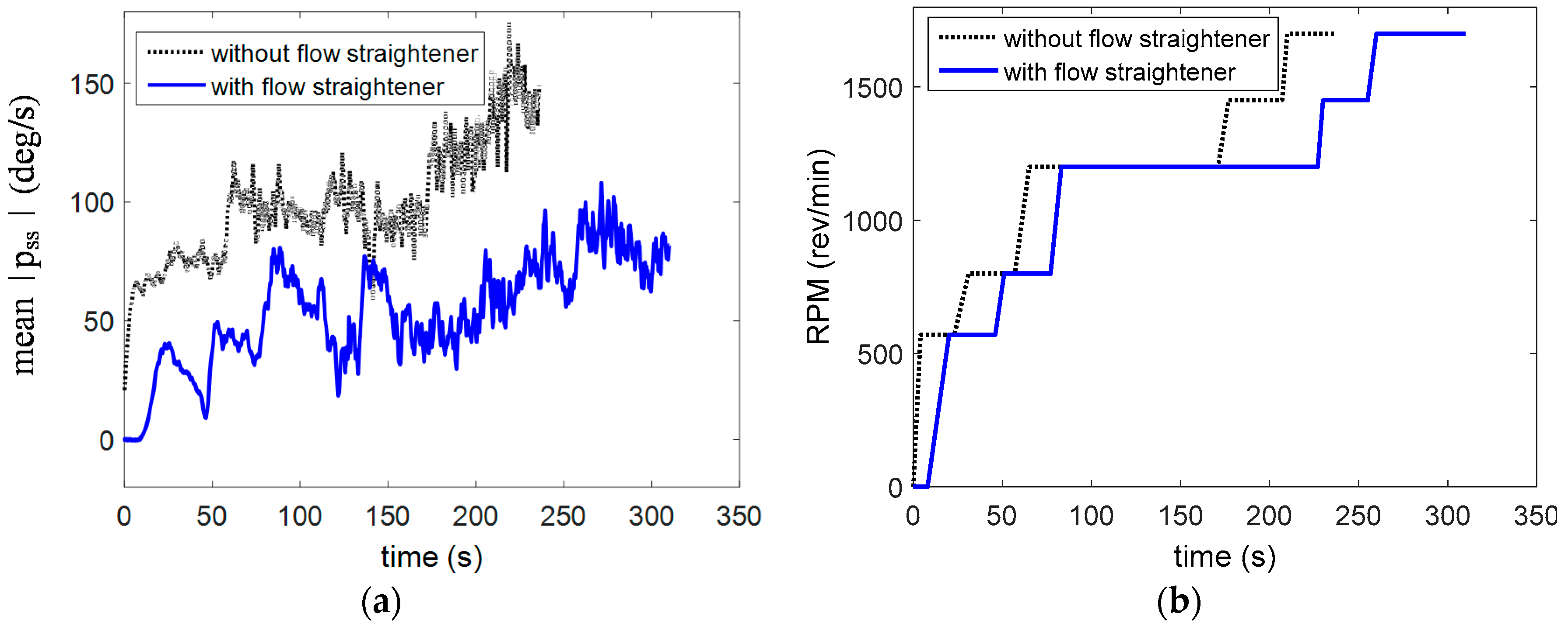
To demonstrate the quality of the flow over time, in the wind tunnel, a Kestrel 4500 wind sensor [18] was placed 200 mm from the edge at the bottom of the door in Figure 1. This position was fixed throughout the experiment. This sensor measures every 2 s and outputs a wind speed measurement rounded to the nearest 0.1 m/s. A finer resolution wind sensor with a higher frequency was not required for this analysis, since wind speeds less than 0.1 m/s have a negligible effect on rocket dynamics. In addition, turbulence properties are independent of the time scale so this test is adequate to characterize the turbulence intensity in the wind tunnel. The revolutions per minute (RPM) reference on the fan was set to a sequence of values defined by:
R P M r e f = [ 570 , 870 , 1100 , 1400 , 1650 , 1700 ]
Taking into account the controller time constant, the times when the fan reaches steady state are:
T R P M = [ 100 , 230 , 390 , 550 , 718 , 858 ]    ( s )
The measured wind speed is shown in Figure 10. At each steady state there are only very small oscillations, showing that the flow is close to laminar. Figure 11a shows a plot of the RPM versus wind speed and Figure 11b plots the turbulence intensity Γ versus wind speed which is defined:
Γ ( v ) = σ 2 ( v ) mean ( v ) , σ standard deviation ,    v wind speed
There is a correlation of R2 = 0.9999 for RPM versus wind speed, thus the fan controller is creating a very linear response. The turbulence intensity is very low and less than 0.04% over all wind speeds tested.

4.1.2. Swirl

It was noticed that in every airframe tested in the wind tunnel, there was a roll rate with the canards set to 0. However, it was not initially known what percentage was of this roll rate, caused by fin offsets in the airframe or swirl in the wind tunnel. To characterize the swirl, several sets of aluminium fins were machined to provide a baseline where there was no fin offset. The fins were made from two thin sheets of aluminium formed in a cross. These fins were attached to a steel pipe and suspended by string in the wind tunnel as shown in Figure 12. Tests showed that the roll rate observed was highly dependent on the total diameter of the fins. For a diameter less than 100 mm, there was no roll rate and greater than 300 mm the roll rate was very low. This result suggests that the swirl is mainly isolated to a concentric ring between 100 and 300 mm from the centre of the wind tunnel. The fin set that was chosen for detailed analysis had a diameter of 200 mm which maximized the roll rate.
The first test was to take a video of the 200 mm aluminium fin rocket for 5 min at the maximum wind speed of 30 m/s and visually count the number of revolutions to work out the average roll rate. The result was 87.0 deg/s which demonstrates there was certainly a relatively significant swirl in the wind tunnel. To overcome this swirl, an egg crate was placed up to a height of 20 cm in a hexagon shape on the grill at the bottom of the wind tunnel, just above the fan, as shown in Figure 13. This egg crate effectively provided an additional flow straightener reducing the swirl as it was near the fan which caused the swirl. Another video was then taken of the aluminium fin rocket and the average roll rate observed was 25.7 deg/s which is a 340% reduction in the swirl. There were also several periods where there was no roll rate.
To fully characterize the impact of the flow straightener with various wind speeds on the Tasha III rocket, an uncontrolled airframe with the same dimensions as Figure 8b was placed in the wind tunnel. This airframe was primarily used to test the parachute before implementing the controlled launch, so had slightly different back fins as a result of natural manufacturing variations, but was essentially the same rocket. The specific rocket in Figure 8b was not available for this test as the back fins were damaged on landing due to swinging into rocky ground with a large gust of wind, just as it landed.
The canards were set to 0 and roll rate data logging was enabled. Figure 14a plots the roll rate response for two experiments with and without the flow straightener. The RPM inputs used in each experiment are plotted in Figure 14b. Figure 14a shows that the flow straightener has significantly reduced the roll rate of the rocket. The mean absolute steady state roll rate for the two experiments were plotted against the corresponding mean steady state velocity in Figure 15.
As a final analysis of these experiments, the effective steady state fin offset is computed using known values of the damping α and torque constant β of the airframe as discussed in the next section. Specifically, at steady state, the roll rate p ˙ , so assuming that u f i n , s s = 0 , the disturbance in Equation (2) can be solved to yield:
u f i n o f f s e t = α p s s β v s s
where “ss” refers to the steady state value for each steady state wind speed v s s which is computed from the average of the velocity during the steady state period of interest. This analysis allows a characterization of the swirl in terms of the effective canard angle. Note that the canards and extra fin area in Tasha III, as well as a larger diameter airframe would cause significantly more damping in Tasha III than in the aluminium fin rocket of Figure 12. Therefore, it’s reasonable to assume that the very small amount of swirl remaining after the addition of the flow straightener would have a negligible effect on the Tasha III rocket. The aluminium fin rocket also has a very low moment of inertia, so the threshold of torque required to overcome the damping in the fins, would be much lower in this rocket and thus much more sensitive to swirl than Tasha III.
A plot of u f i n o f f s e t versus v s s or both experiments, is given in Figure 16. This figure shows that in the case of no flow straightener, the swirl has a greater effect at the lower velocities. This result was expected since the vertical component in the wind tunnel would not be sufficiently high to overcome the horizontal component induced from the swirl. However, with the flow straightener there was very little difference in the fin offset over all velocities, which provides further evidence that there is negligible swirl in this case. Subtracting the two curves in Figure 16 provides a measure of the swirl in terms of the effective canard offset. After 20 m·s−1, there is an average of about 2° of swirl in the wind tunnel. This value will need to be subtracted from future tests to get a better estimate of the true fin offset for flight prediction.

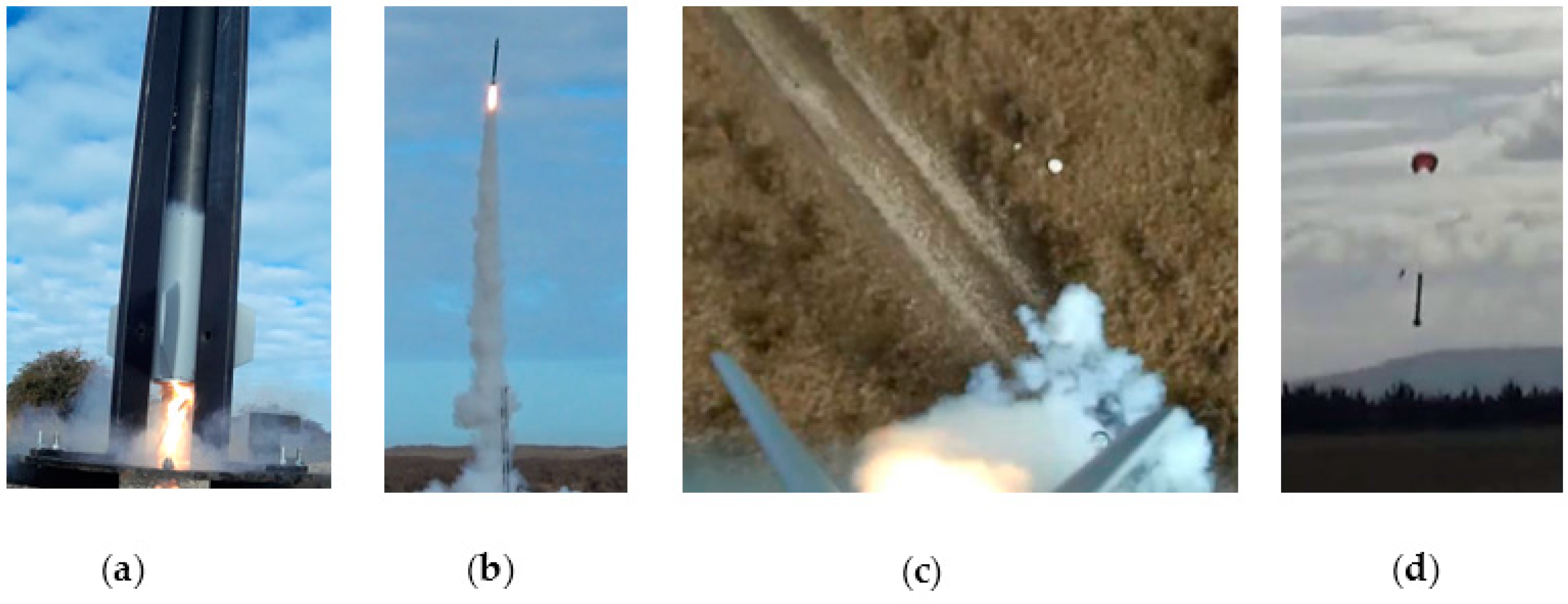
4.2. Tasha III—Launch 1

Tasha III from Figure 8b was launched from Kaitorete Spit on 22 July 2015. The aim of this launch was primarily to test the new avionics stack and fibreglass rear fins. In the previous flight of Smokey [12], the fins were 3D printed. The reason for the fibreglass was to provide further strengthening suitable for supersonic flights in future research. In addition, to gain some useful data from the launch, a PD controller was implemented during flight in both the thrust and coast periods. Since the vehicle was finished only days before the launch, there was not sufficient time to do a full wind tunnel test, analysis of data and rigorous testing of gains. The only wind tunnel test performed was the stability test of Section 3.2.
For the flight, the gains chosen were k p = 1 , k d = 0.1 , which were known to give a reasonable response from previous wind tunnel testing of Smokey with the gimbal frame [12]. The reference was chosen to be a series of responses starting at 0° for a pre-determined amount after clearing the launch guide, followed by an alternation between −15° and 15° every second. As a precaution, since this was the first flight with the avionics, a maximum limit of 6° was enforced in each canard. Unfortunately, there was a significant fin offset in the airframe which was greater than the canards could compensate for with this maximum limit, so only about 1 s of oscillatory data was obtained. However, this data set was sufficient to identify parameters and thus analyse the rocket roll response.
The apogee for this flight was 522 m, the time to apogee was 10.2 s and the maximum velocity was 97 m·s−1. The wind speed was very low on the day, varying between 1 and 2 m·s−1 on the ground. The flight was successful and the rocket safely recovered apart from a couple of broken canards that were easily replaced. Figure 17 shows video stills from the ignition, take-off, onboard footage and parachute recovery.
Since there was only one step response from 0° to −15°, the control reference is modeled by a single Heaviside function and the proportional derivative (PD) control command is defined:
u c m d = max { min { u ^ c m d , u m a x } , u m i n } H ( t T P D )
u ^ c m d = k p ( R ( t ) ϕ ( t ) ) + k d ( R ( t ) p ( t ) )
R ( t ) = R 0 ( R 0 R 1 ) H ( t T P D 1 )
u m a x = 6 π 180 , u m i n = 6 π 180 , R 0 = 0 , R 1 = 15 π 180 , k p = 1 , k d = 0.1 , T P D = 0.42
The Heaviside function in Equation (28) provides a delay of T P D after the launch detect to ensure the rocket is well clear of the launch guide before starting control. For launch detection to occur, the on board accelerometer on the rocket’s vertical axis needs to detect a consistent 2 g or higher acceleration over 0.2 s. This requirement prevents sensor errors or motor misfires from triggering launch control. Once the launch is detected, the rocket’s vertical axis acceleration is transformed to the earth reference frame and then double integrated to determine the rocket’s height above the launch guide. Using the two conditions of launch detection and launch guide clearance enables safe conditions for actuating the rocket’s canards.
The roll rate data including all the key points of the launch are given in Figure 18, where t = 0 corresponds to 1.5 s before launch. The control was started when the rocket height was 2 m above the 4 m launch guide. However, due to the specified 0.2 s delay in the launch detect, the actual altitude when control started was 7 m which was 0.63 s after lift-off.
The commanded and encoder measured canard roll angle are defined as the average of all canard inputs which is standard in the literature [19]:
u c m d = c m d 1 + c m d 2 + c m d 3 + c m d 4 4
u e n c = e n c 1 + e n c 2 + e n c 3 + e n c 4 4
The data is analyzed from just before control starts up to a couple of seconds before the parachute deployment. The roll rate and fin angle u e n c which is computed from Equation (33) using the encoder outputs e n c 1 , , e n c 4 for each canard, are plotted in Figure 19, where the time is reset to 0. Note that for some of the thrust period and all of the coast period all the canards are set at their maximum values of 6°, yet the roll rate stays negative. The reason is there is a fin offset which is larger than the 6° that the canards can compensate for.
To identify the torque constant β, damping α and disturbance u d i s t ( t ) from the roll model of Equations (2)–(8), the first step is to specify the range in the β and α values as given in Equation (19). These ranges are defined:
α = { 1 , 2 , , 60 } ,       β = { 5 , 5.5 , 6.5 , 7 , , 15 }
The next step is to define the time values for the disturbance changes in Equation (7). These values are equally spaced in both the thrust period and the coast period of the data which are denoted in Figure 19a. Let N thrust be the number of time points in the thrust period and N c o a s t the number of time points in coast period. The values in Equation (7) are defined:
T i = i T t h r u s t N t h r u s t ,     i = 1 , , N t h r u s t
T N t h r u s t + j = T t h r u s t + j ( T e n d T t h r u s t ) N c o a s t ,    j = 1 , , N c o a s t
Since there are no dynamics in the canards during coast, N c o a s t is set to the minimum possible value which obtains a reasonable match in the coast period. It was found empirically that higher values than 2 do not help identifiability due to the lack of dynamics during this period, and a value of 1 gave a consistently large error. Therefore N c o a s t is set to 2 for all the analysis on this launch. The value of N t h r u s t was also minimized and it was found that N t h r u s t = 2 was also a good choice. Higher values gave a progressively better match to the data in the thrust period as would be expected, but were much slower computationally. Specifically, the values from N t h r u s t = 2,⋯,6 gave virtually identical results with an improvement in the match to the roll angle by less than 0.1°. More importantly, the identified damping remained unchanged and the torque constant only varied by a maximum of 0.05. The results for N t h r u s t = 2 and N c o a s t = 2 are defined:
α b e s t , O L = 8.5 , β b e s t , O L = 10.0
μ | p | , O L mean absolute error in roll rate = 9.82  deg / s 
μ | ϕ | , O L mean absolute error in roll angle = 1.51  deg / s 
The model response is plotted against the measured values for both the roll rate and roll angle in Figure 20. A zoomed in plot of Figure 20a is given in Figure 21a and the identified time-varying disturbance is plotted in Figure 21b.
Figure 21a shows that although there is some error in the first controlled response, the overall trends are captured accurately. For example the data drops 27.2° from the local maximum at t = 0.49 s to the local minimum at t = 1.02 s where the model predicts a drop of 26.15° which corresponds to less than 4% error. The model also captures all the coast period, in both the roll angle and roll rate, as shown in Figure 20. The disturbance is quite low initially in the first 0.5 s of the data. This behavior is caused due to low velocity and therefore the canard–fin disturbance dominates the dynamics, as the fin offset takes some time to take effect. After about 1 s the disturbance rapidly converges to a near constant value around −7° which remains for the rest of the flight with only a minor increase at the end. The results of Figure 20 and Figure 21 and Equations (38) and (39) show that quite a simple model with a relatively smooth disturbance function, is very effective in capturing the rocket roll response.
Note that the second PD controlled roll response in Figure 21a has a very large steady state error, since the reference was −15°. The reason for this error is that the fin offset is having a major effect due to the increased velocity and the maximum and minimum canard constraints do not provide enough actuation to overcome this fin offset. However, the goal of this launch was not control, but to test the logistics of the new launch vehicle and avionics and provide an initial proof-of-concept of the model and methods.
The final validation of the model and methods for this launch is to match the closed-loop model of Equations (28)–(31) to the data. The results are:
α b e s t , C L = 7.5 , β b e s t , C L = 10.0
μ | p | , C L mean absolute error in roll rate  = 9.76  deg / s 
μ | ϕ | , C L mean absolute error in roll angle  = 1.50 deg
These results are very close to the open-loop response with a mean error difference of 0.06 deg/s in the roll rate and 0.01° in the roll angle. However, there are some small differences in the thrust period in the roll angle as shown in Figure 22a, but the overall behavior of the two responses are very similar. In addition, apart from a small period in the thrust, the identified closed and open-loop disturbances are virtually identical as shown in Figure 22b.
Hence, in summary, there is no noticeable change in the output responses and identified parameters when using the closed-loop model over of the open-loop model, although the closed-loop model typically takes about 50% longer to simulate. The advantage of the open-loop model computationally is that the roll rate is decoupled from the roll angle which is simpler to handle numerically.

4.3. Tasha III—Launch 2

A new vehicle was manufactured for the second launch including fibreglassing the rear fins and 3D printing two new canards to replace the ones that were broken during the Tasha III launch 1, see Figure 8c. For this vehicle, a number of controlled step responses were performed in the wind tunnel shortly before the launch. Hence, there is a good amount of data to identify torque, damping and disturbances and to analyze the capability of the wind tunnel tests to predict flight response.

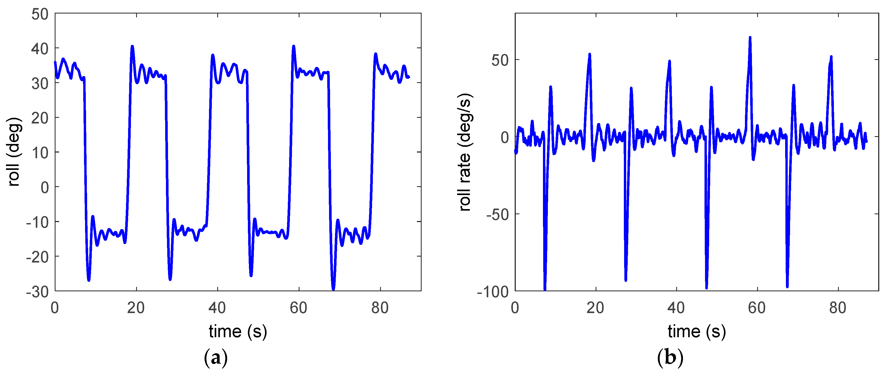
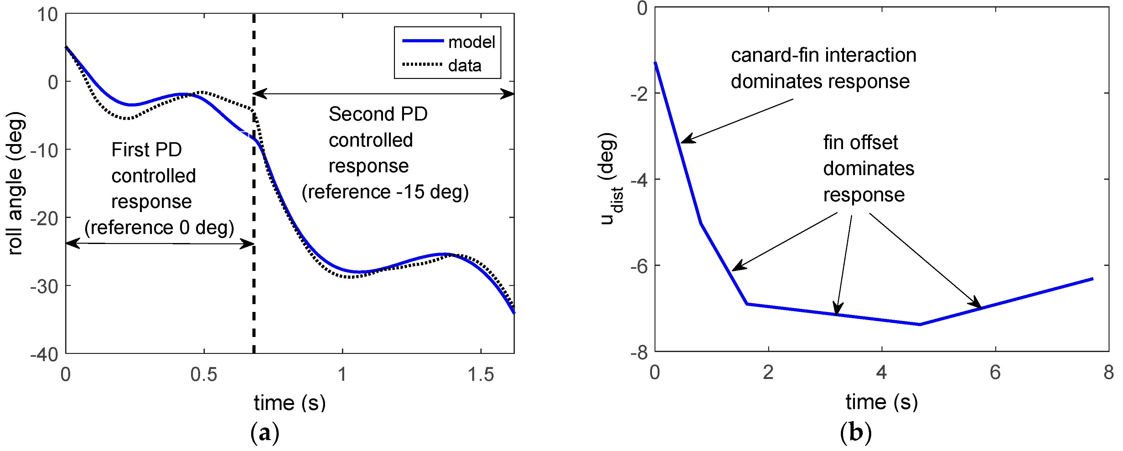
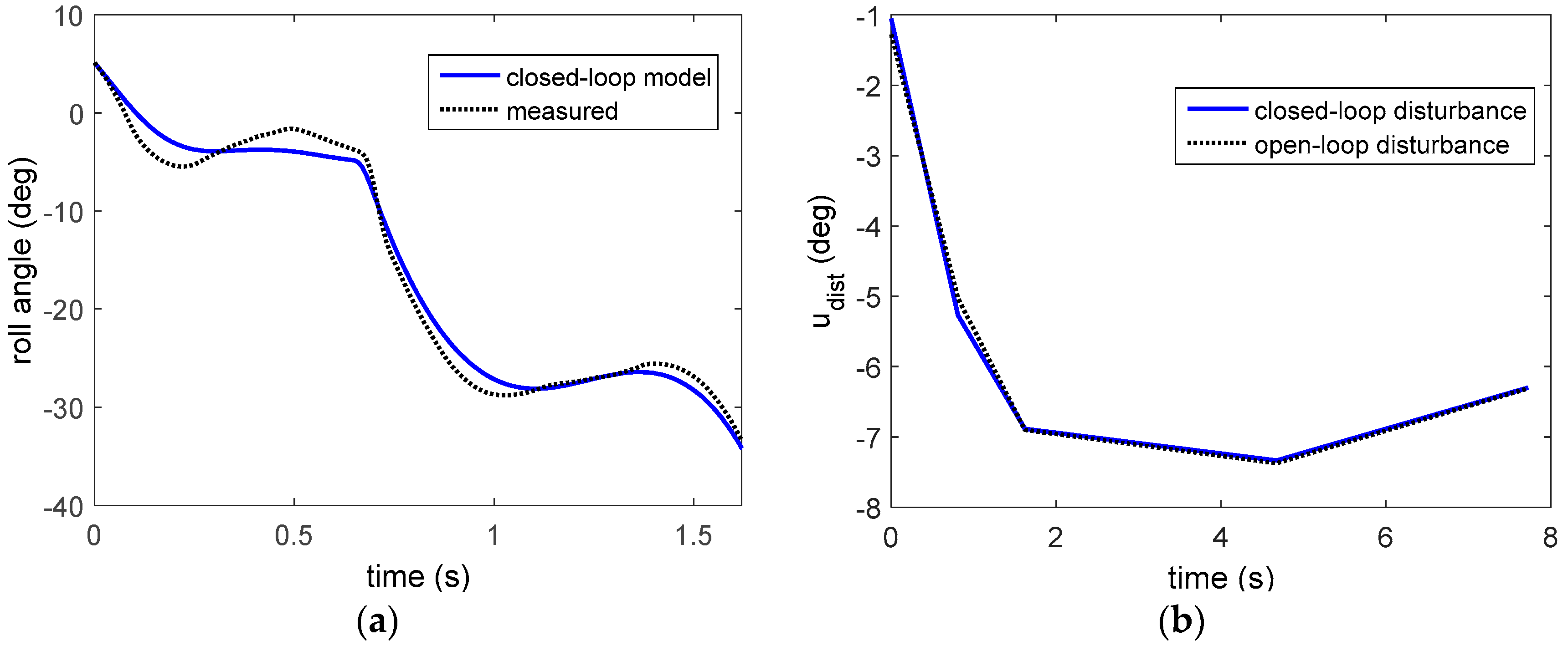
4.3.1. Wind Tunnel Step Responses
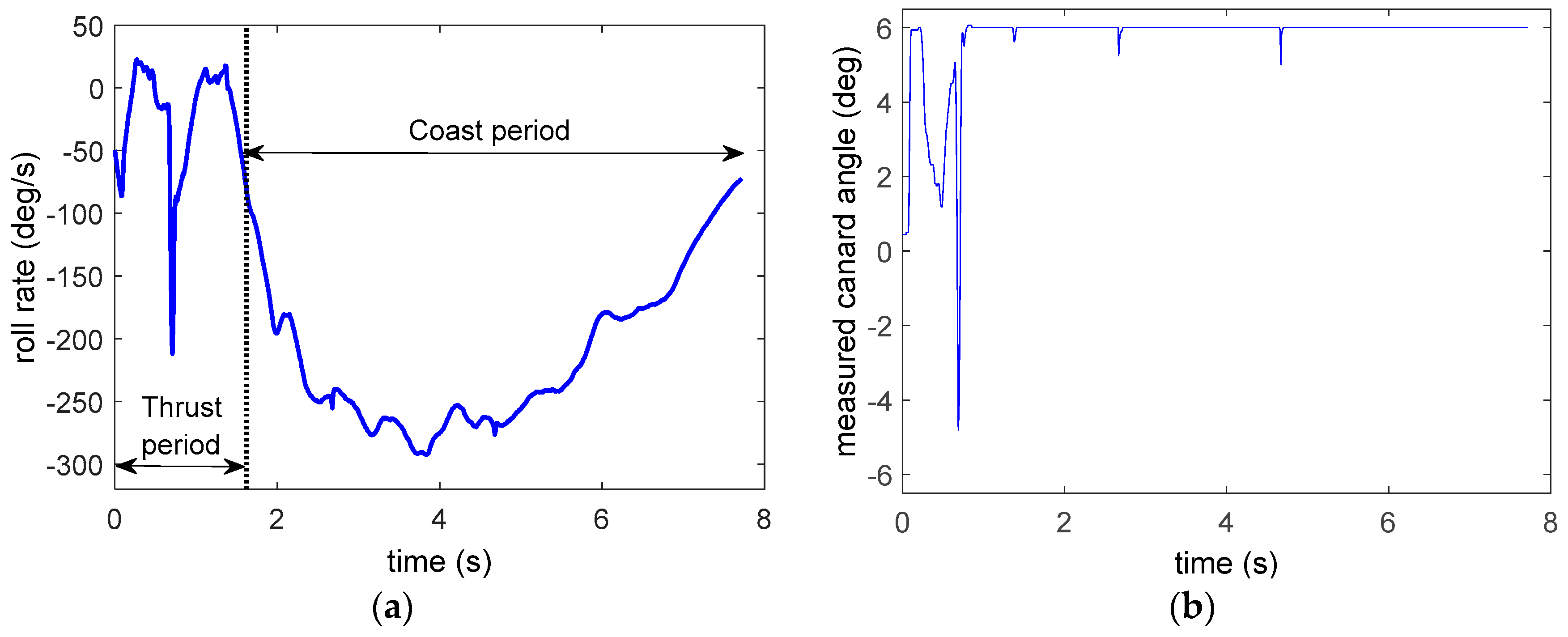
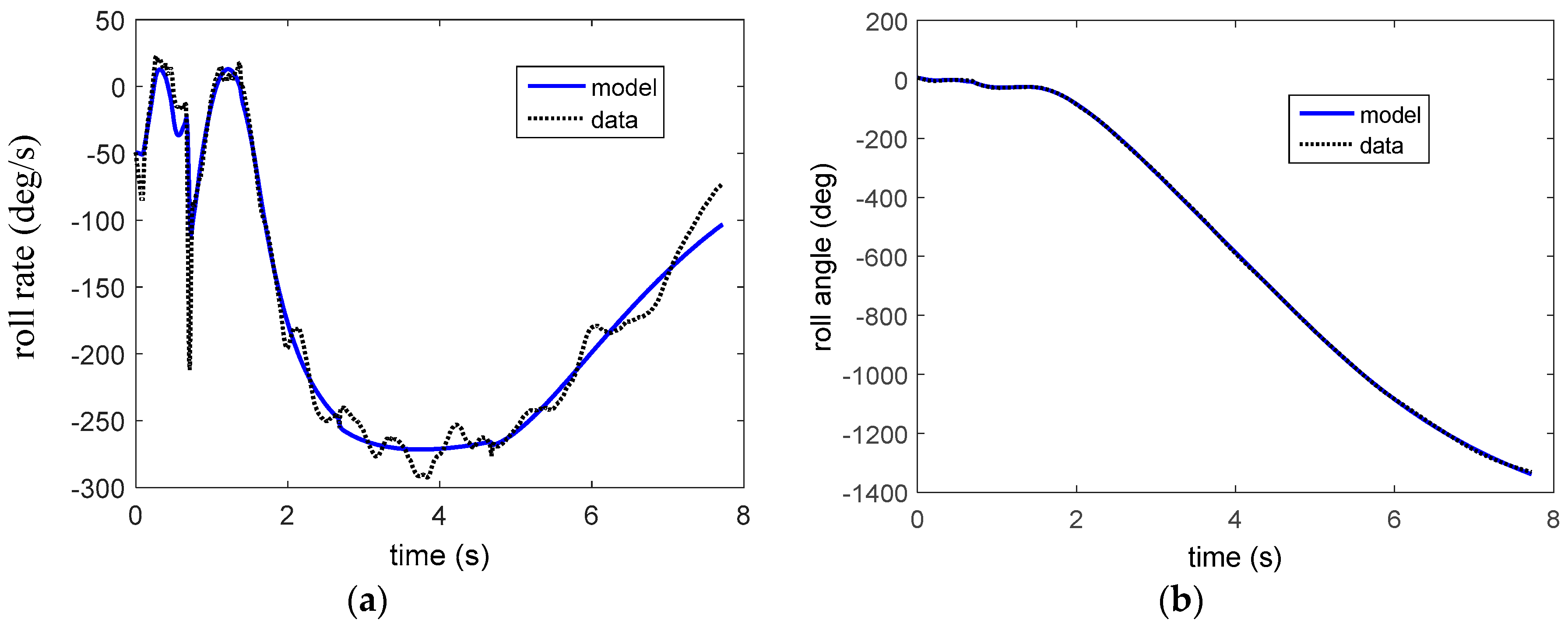
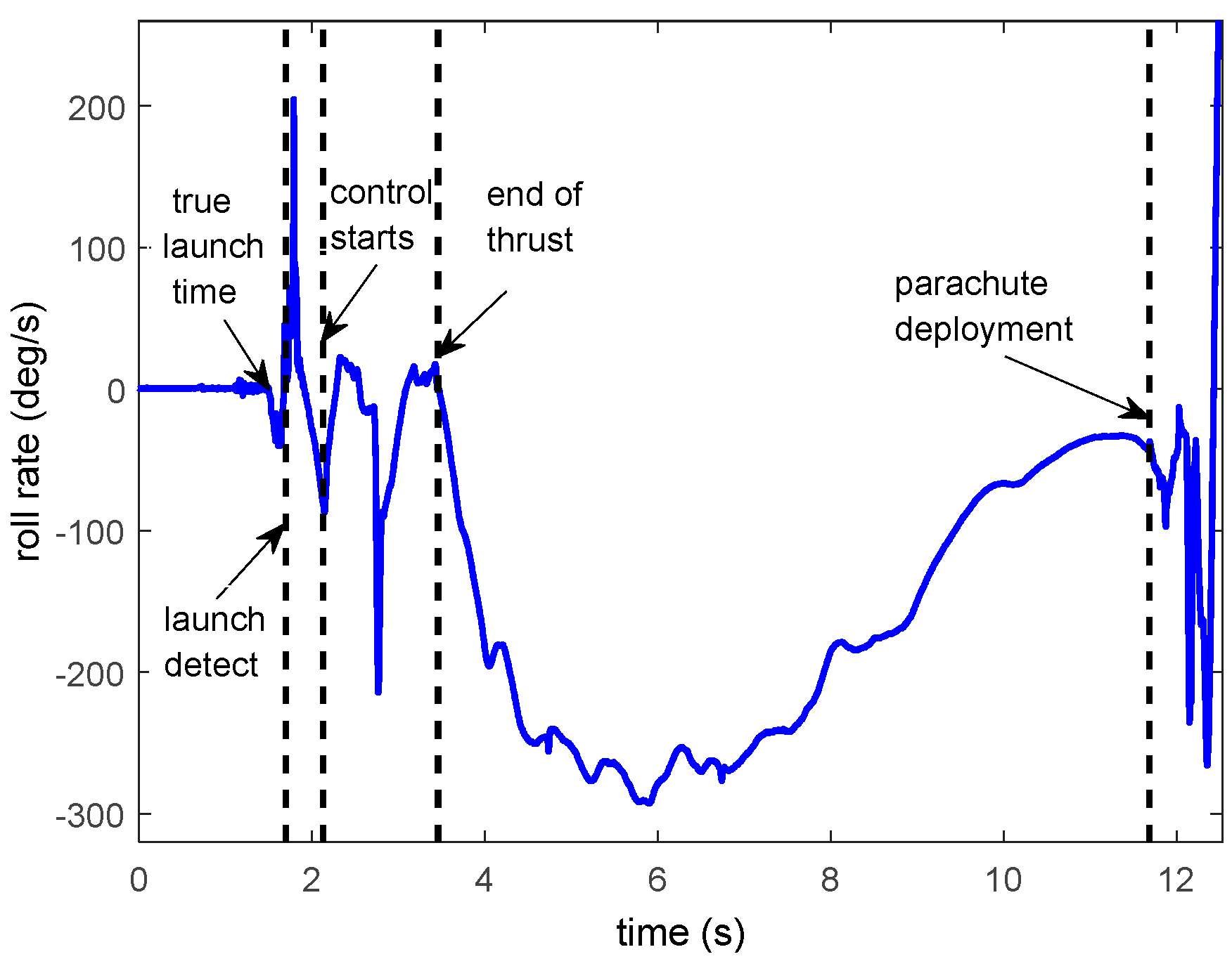
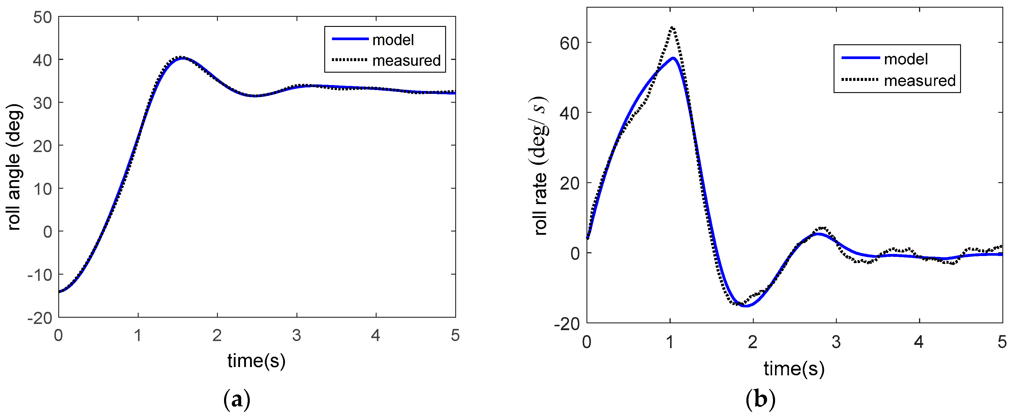
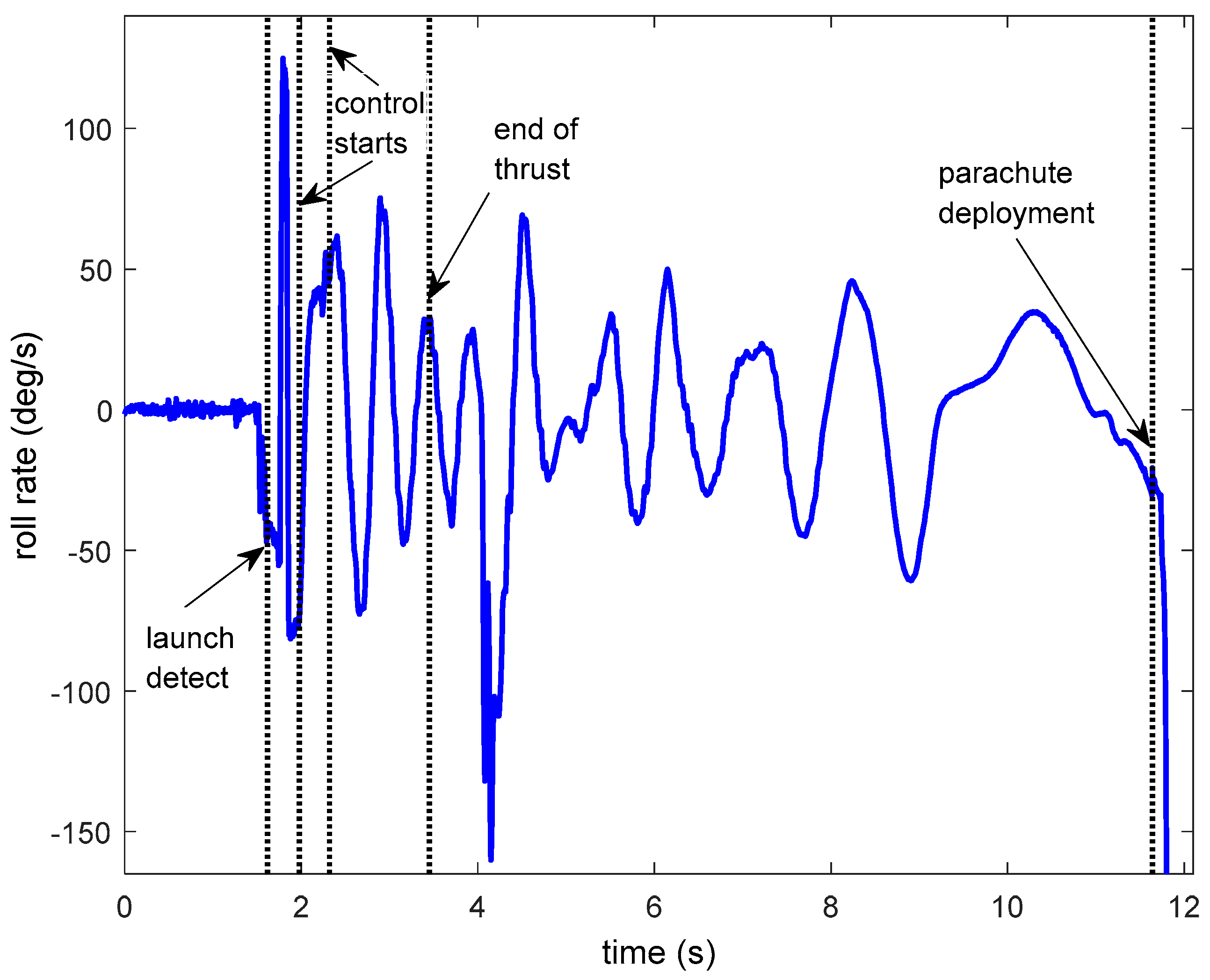
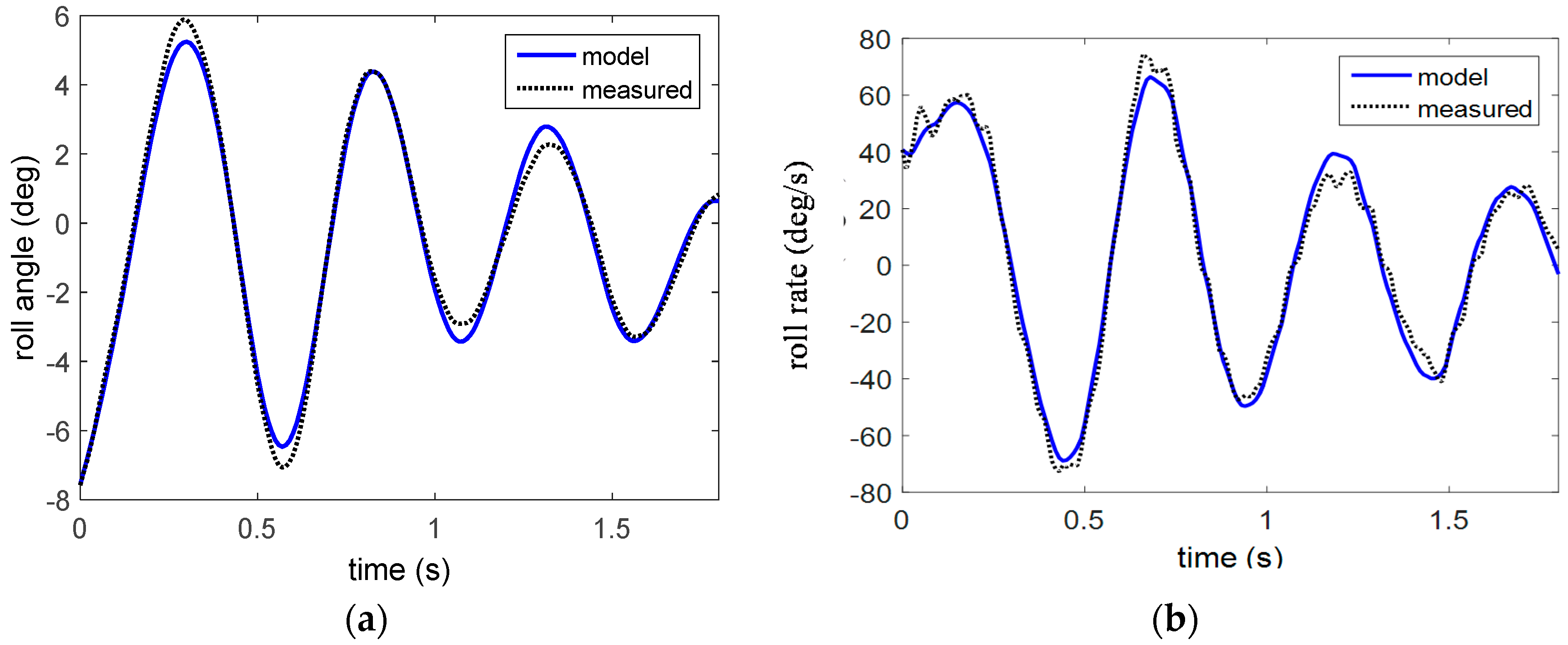
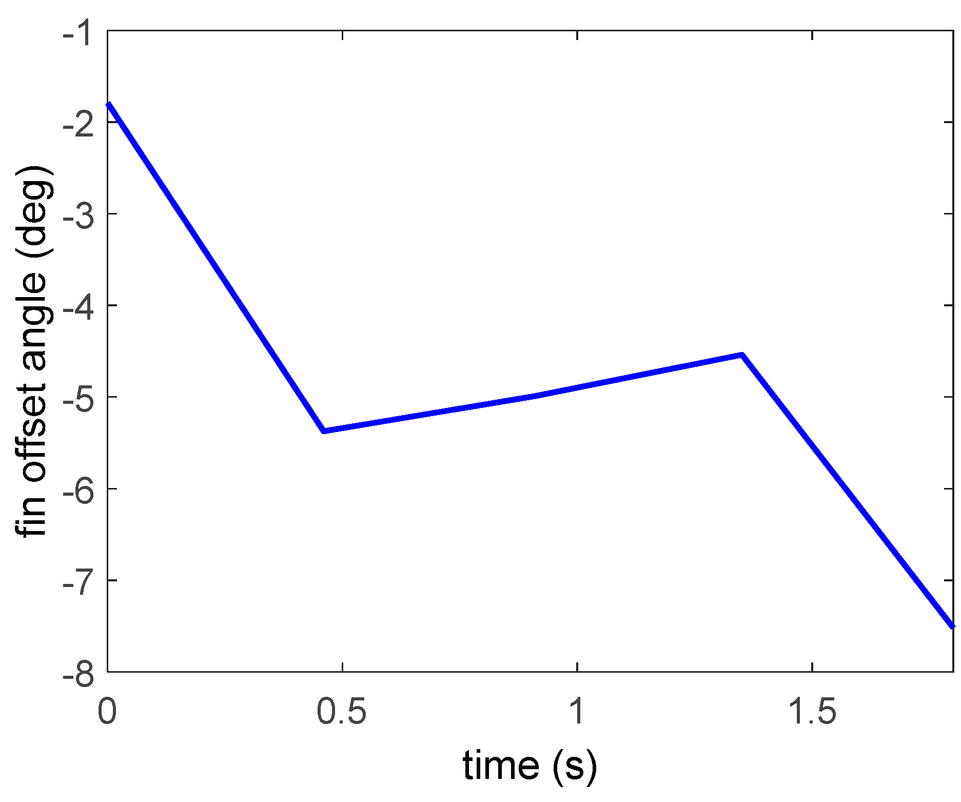
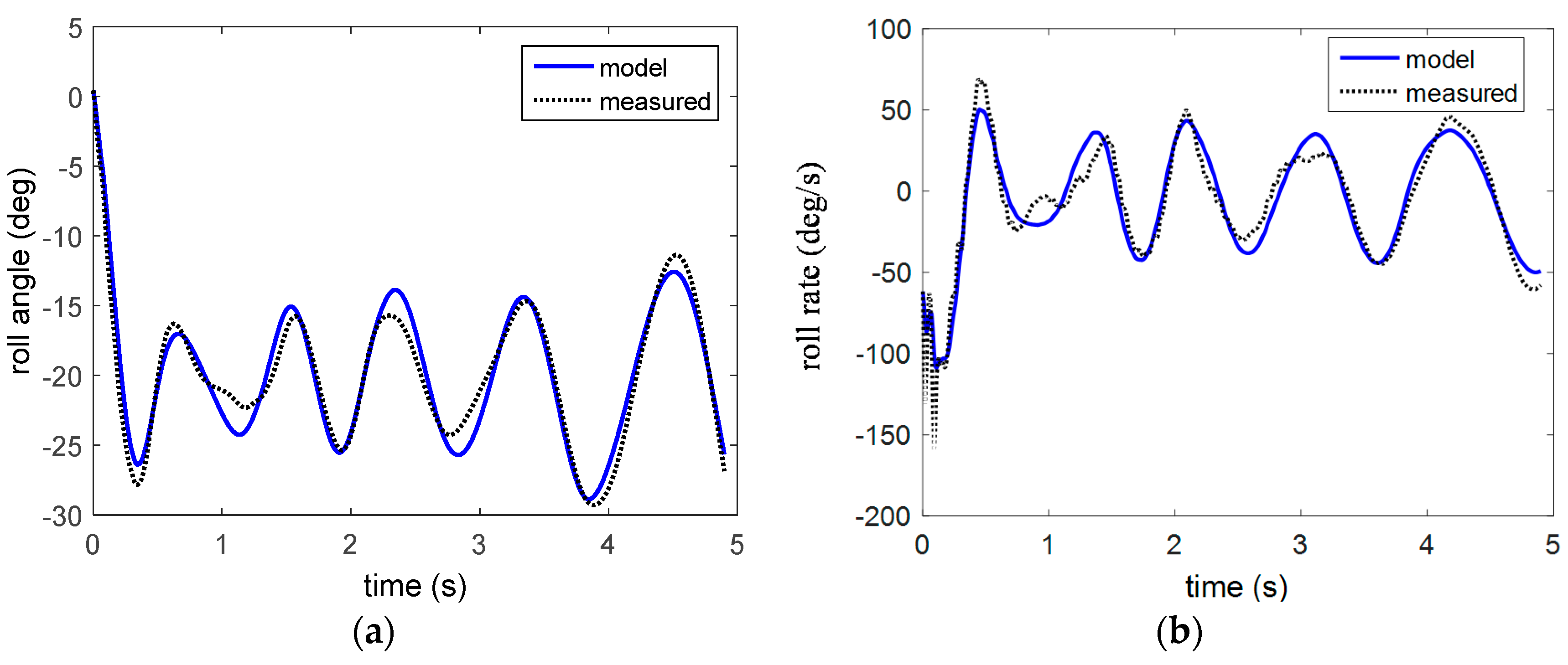
The rocket was suspended from a string, and 8 step responses were performed with a magnitude of 45°, at a wind speed of 22 m·s−1. The highest wind speed of 30 m·s−1 was not used in this case, as it was found that this airframe also had a fin offset, so it was spinning rapidly and starting to swing backwards and forwards, risking damaging the canards. The gains and frequency were reduced and the parameters in Equations (11) and (12) are defined:
k p = 0.5 , k d = 0.05 , f 0 = 0.1 , R 0 = 45 π 180 , R 1 = 0
The roll angle and roll rate responses are plotted in Figure 23.
Figure 23 shows there are significantly different overshoots and rise times for each step response as well as a major difference in dynamics depending on the direction of rotation, which is likely caused by the fin offset in the airframe. To account for these variations, the model of Equations (2)–(12) is identified for each individual step response. Since the oscillations reduce quite quickly after the first peak, only the first half of the data in each step response is used for the parameter identification. The remaining half is essentially disturbances in the wind tunnel, and there are very few canard dynamics so it does not contribute to identifiability. The time points in the disturbance model of Equations (4)–(8) were chosen to be simply the beginning and end points with N = 1 in Equation (4). Since 5 s is analyzed in each data set, and time is reset to 0 each time, the time points are defined:
T 0 = 0 , T 1 = 5
For the grid search and non-linear regression algorithm, the ranges of the parameters are taken from Equation (34). The results identified parameters and mean model response errors for the open-loop model of Equation (9) are given in Table 2. An example set of model responses is plotted in Figure 24, which is the sixth step response in Figure 23. Both the roll angle and roll rate match very closely to the measured data, even with a very simple linear model, for disturbance across the whole data set considered.
Table 2 shows there is a significant variation of parameters across the step responses. The average model error over all tests was 0.88° and 3.52 deg/s for the roll angle and roll rate respectively. The size of the step response was 45°, so the average model errors in Table 2 vary from 0.6% to 3.6% of the change in roll angle. Hence, the model and methods are very effective at capturing rocket roll response in the vertical wind tunnel. The disturbances in column 4 of Table 2 show a trend for a lower disturbance in the first period, which was similar to the flight in Figure 22b, showing that the canard-fin interaction effects can minimize the effect of fin offset in the airframe. The average fin offset across all tests was −6.1°, so taking into account the swirl this value corresponds to −4.1°. The wide range of values of the damping, torque constant and fin offsets in Table 2 give the range of uncertainty in the launch, and will be compared with the flight data in the next section.

4.3.2. Flight Data

Tasha III from Figure 8c was launched from Kaitorete Spit on 4 December 2015. The aims of this launch included testing the rocket under a greater amount of actuations and to overcome the fin offset problem that occurred in the July launch as detailed in Section 4.2. Importantly, the launch provided a characterization of the ability of the wind tunnel to predict flight dynamics far outside the wind speeds that can be generated by the fan. Since the wind speed for the wind tunnel data was only 22 m·s−1, this launch provided a rigorous test of how well the model could be extrapolated to higher wind speeds. The apogee for this flight was 422 m, and the maximum velocity was 81 m·s−1 which were much lower than the July launch, due to the increased weight from the more robust, supersonic capable avionics stack. The wind speed was reasonably low on the day with an average ground speed of 3 m·s−1. Figure 25 shows several stills of the rocket moving up and leaving the launch guide. The overall launch was a success although the back fins were damaged on landing, due to a sudden gust of wind that pushed the rocket onto stony ground.
The controller for this launch was a single step response from 0° to −20°, which occurred 2 s after the controller was switched on. The canard limits were increased to ±9° in this launch to overcome the fin offset from the first launch. In addition, some open-loop oscillatory inputs were included in the PD control signal of Equation (10). This input signal was implemented 0.4 s after the control started and was stopped 5 s after the −20° step response. The input was a modified chirp signal defined:
u i n p u t ( t ) = ( A 0 + Δ A ( t ) ) sin ( ( ω 0 ( t ) + Δ ω ( t ) ) t )
A 0 = 4 π 180 ,    ω 0 ( t ) = 2 π ( 2 t 10 ) ,    Δ A ( t ) , Δ ω ( t ) random variation on signal
A plot of the applied input signal is given in Figure 26.
The roll rate data including all the key points of the launch are given in Figure 27, where t = 0 corresponds to 1.5 s before take-off. For this launch, two accelerometers were used to improve the robustness in the launch detect and the delay threshold was reduced to 0.1 s. In addition, the accelerometer threshold increased to 2.5 g. Similarly to the Tasha III launch 1, the control was started when the rocket height was 2 m above the 4 m launch guide.
For this launch, the data is split into the two PD controlled responses with the set point of 0° followed by −20° which was 2 s later. A sharp change in roll rate can be seen for this second set point at about 4 s in Figure 27. The first period of analysis is started at 2.4 s in Figure 27 which is 0.4 s after the control starts and corresponds to the implementation of the input signal from Figure 26. This starting point was chosen since there are significant oscillatory dynamics in the canards which will ensure good identifiability of the model parameters. The second period of analysis starts at 4 s in Figure 27, which is when the set point changes from 0° to −20°.
For the first period, a similar approach to the Tasha III launch 1 model is applied, where N1 equally spaced points are chosen, and N1 is increased until there is no significantly further improvement in the fit to the data. The values of N1 investigated were from 1 to 6 points. For N1 = 1,⋯,4, the best model fits had average roll angle errors of 2.36, 2.15, 0.57 and 0.26° respectively. There was no significant improvement for N1 = 5 and 6 and the parameters remained virtually identical for N1 = 3,⋯,6. Hence a value of N1 = 4 is chosen for the final model. The results are defined:
α b e s t , O L = 23.0 , β b e s t , O L = 9.0
μ | p | , O L mean absolute error in roll rate = 4.10  deg / s
μ | ϕ | , O L mean absolute error in roll angle = 0.26  deg / s
The model response for the roll angle and roll rate are shown in Figure 28 and the offset angle is plotted in Figure 29.
The results of Equation (47) are close to the average wind tunnel predicted values of 19.4 and 9.6 in Table 2, with errors of 15.7% and 4.4%, respectively. The offset angles in Figure 29 are all within the range of values of the wind tunnel tests as well. There is also a similar trend of lower offset angles for the smaller fin movements as was the case in the wind tunnel. The mean offset angle of Figure 29 was 4.9° which is 0.8° greater than the average of 4.1° predicted in the wind tunnel. This value corresponds to an error of 16.3% but well within the expected variation of Table 2.
A similar procedure was applied to the second period of data corresponding to a reference angle of −20°. In this case, a value of N2 = 2 was sufficient for the modelling and the identified parameters are defined:
α b e s t , O L = 23.0 , β b e s t , O L = 9.0
μ | p | , O L mean absolute error in roll rate = 8.32  deg / s
μ | ϕ | , O L mean absolute error in roll angle = 0.99  deg / s
The model responses for the roll angle and roll rate are shown in Figure 30 and the offset angle is plotted in Figure 31.
The modeled torque constant in Equation (50) is reasonably close to the wind tunnel predicted value of 9.6 with an error of 16.7%, however the damping is significantly larger than all the damping values of Table 2. This extra damping is likely due to the rocket pitching over with an increasing angle of attack as well as the higher velocity. On the other hand, the average identified offset of Figure 31 is −4.7°, which is even closer to the wind tunnel average of 4.1°. Hence, although the damping is less accurate in the post-thrust period, the torque constant and the offset angles are both accurately predicted for all stages of the flight, which are more important for control design. A similar analysis has been performed for the closed-loop responses, but since the results were very similar to the open-loop analysis above, these results are not shown.
Note that the torque constant values of β = 8 and β = 9 in this second Tasha III launch are reasonably close to value of β = 10 identified in the first Tasha III launch. However, both of the values of damping in the second launch are considerably larger than the damping from the first launch. This result is probably because there were a lot less dynamics in the first launch so the damping was less identifiable.

5. Conclusions

A vertical wind tunnel has been designed and built at the University of Canterbury. This wind tunnel has been specifically customized for sounding rocket research and has a unique feature of allowing the rocket to be suspended by string for accurate prediction of roll dynamics. It is also very useful for testing stability before flight. The flow of the wind tunnel was analyzed in detail and turbulence intensity was estimated to be less than 0.04%. However, there was a reasonable amount of swirl equivalent to 2° of canard fin. This swirl was dramatically reduced to a negligible amount by using an egg crate at the bottom of the wind tunnel near the fan to straighten the flow.
Two new airframes were developed in this research with a supersonic capable avionics stack in the second vehicle. Both rockets had reinforced fiberglass to give strength to the fins, but it was found that they had significant fin offset, with post-thrust average values of about 7° for the first vehicle and 5° for the second. Wind tunnel tests on the second vehicle revealed a high roll rate, which suggested a combination of swirl and fin offset. After the second flight, tests with and without the flow straightener using a similar airframe, showed that swirl could be modeled by the equivalent canard offset. This value was then used to compare the wind tunnel tests of the second vehicle to the flight data.
A minimal modelling approach for roll dynamics was developed using a velocity dependent model and a piecewise-linear time-varying canard offset function. Open and closed loop models were considered with PD control, with encoders used to measure the canard movements. A combination of a grid search and non-linear regression provided a rigorous way of identifying the parameters. The models identified gave an excellent match to the flight data in both launches, with quite a smooth varying canard offset profile. It was found that with high dynamic movement in the canards the identified fin offset was lower, showing that canard–fin interaction dominates during these periods. This phenomenon occurred in both the wind tunnel tests and flight.
A significant outcome of this paper was proving that wind tunnel tests give accurate predictions of the torque constant and fin offset and importantly, the resulting minimal roll models predict flight behavior closely. The damping is typically underestimated in the wind tunnel so a greater uncertainty should be included in this parameter for future control design.
In summary, the vertical wind tunnel at the University of Canterbury is a unique facility and a key part of the success of UC Rocketry. A combination of wind tunnel tests and rocket launches have allowed a thorough understanding of rocket flight and control.

Acknowledgments

Funded by the Rutherford Discovery Fellowship, Royal Society New Zealand; Callaghan Innovation PhD Fellowships; and Rocket Lab Ltd.

Author Contributions

Hoani Bryson, Hans Philipp Sültrop, George Buchanan, Christopher Hann, Malcolm Snowdon, Avinash Rao, Adam Slee, Kieran Fanning, David Wright: developed the hardware, did the experiments, analyzed the data, developed models and wrote the paper. Jason McVicar, Brett Clark, Graeme Harris and Xiao Qi Chen: helped to construct the wind tunnel including setting up the fan and controller, provided expertise and advice on the flow quality and instrumentation and sensors for the wind tunnel tests, and contributed to writing the paper.

Conflicts of Interest

The authors declare no conflict of interest.

Notation

I p
Inertia in roll axis (kg/m2)
ρ
Air density (kg/m3)
α
Damping constant (m2)
β
Torque constant (m)
u f i n
Roll fin angle (rad)
A
Cross sectional area (m2)
p
Roll rate (rad/s)
v
velocity (m/s)
k p , k d
Proportional and derivative gains
R ( t )
Reference angle (rad)
u d , 0 , , u d , N
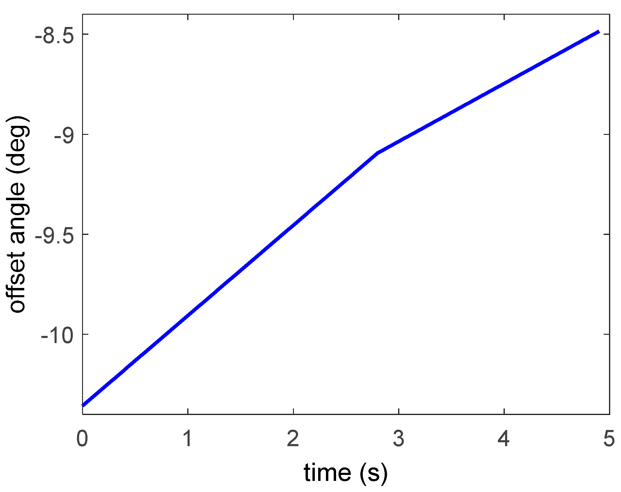
Time-varying disturbance offset angle parameters (rad)
ϕ d a t a
Measured roll angle (rad)
ϕ O L , ϕ C L
Open and closed loop numerical solutions to roll equations (rad)
α , β
Ranges for α, β in the grid search for parameter identification
Γ
Turbulence intensity (m/s)
σ
Standard deviation of wind speed (m/s)
u c m d
Commanded canard angle (rad)
u e n c
Measured canard angle by encoder (rad)
c m d 1 , , c m d 2
Individual canard commands (rad)
e n c 1 , , e n c 2
Individually measured encoders (rad)
u m i n , u m a x
Minimum and maximum canard limits for actuation (rad)
μ | p | , O L , μ | p | , C L
Mean absolute roll rate for open loop and closed loop controllers
μ | ϕ | , O L , μ | ϕ | , C L
Mean absolute roll angle for open loop and closed loop controllers
u i n p u t
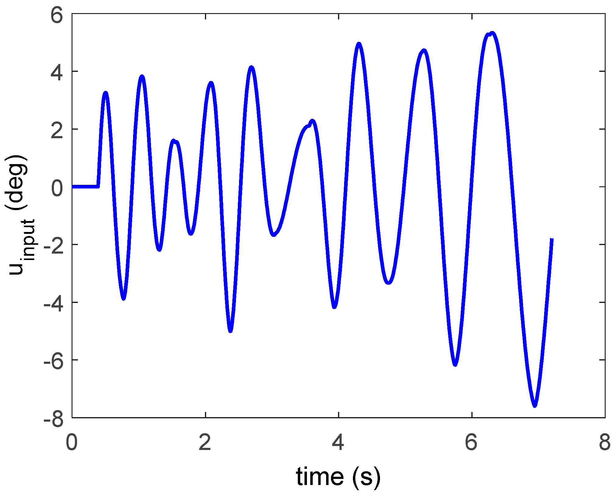
Open loop input signal into PD controller

Abbreviations

PD
Proportional-derivative
NASA
The National Aeronautics and Space Administration
UC
University of Canterbury
CFD
Computational Fluid Dynamics
RPM
Revolutions per minute
OL
Open loop
CL
Closed loop

References

  1. UC Rocketry Project. Available online: http://ucrocketry.org/ (accessed on 1 March 2016).
  2. Schrijer, F.; Bannink, W. Description and Flow Assessment of the Delft Hypersonic Ludwieg Tube. J. Spacecr. Rocket. 2010, 47, 125–133. [Google Scholar] [CrossRef]
  3. Spirito, J.D.; Vaughn, M.E., Jr.; Washington, W.D. Numerical Investigation of Canard-Controlled Missile with Planar and Grid fins. J. Spacecr. Rocket. 2003, 40, 363–370. [Google Scholar] [CrossRef]
  4. Silton, S.I.; Fresconi, F. Effect of Canard Interactions on Aerodynamic Performance of a Fin-Stabilized Projectile. J. Spacecr. Rocket. 2015, 52, 1430–1442. [Google Scholar] [CrossRef]
  5. Curfman, H.J.; Grisby, C.E. Longitudinal Stability and Control Characteristics of a Canard Missile Configuration for Mach Numbers from 1.1 to 1.93 as Determined from Free-Flight and Wind-Tunnel Investigations; Technical Report for NASA Langley Aeronautical Laboratory: Hampton, VA, USA, 1952. Available online: http://ntrs.nasa.gov/archive/nasa/casi.ntrs.nasa.gov/19930087105.pdf (accessed on 1 March 2016).
  6. Dollyhigh, S.M. Subsonic and Supersonic Longitudinal Stability and Control Characteristics of an Aft-Tail Fighter Configuration with Cambered and Uncambered Wings and Cambered Fuselage; Technical Report for NASA Langley Research Center: Hampton, VA, USA, 1977. Available online: http://ntrs.nasa.gov/archive/nasa/casi.ntrs.nasa.gov/19770024149.pdf (accessed on 1 March 2016).
  7. Blair, A.B., Jr.; Hernandez, G. Effect of Tail-Fin Span on Stability and Control Characteristics of a Canard-Controlled Missile at Supersonic Mach Numbers; Technical Report for NASA Langley Research Center: Hampton, VA, USA, 1983. Available online: http://ntrs.nasa.gov/archive/nasa/casi.ntrs.nasa.gov/19830019688.pdf (accessed on 1 March 2016).
  8. Dillenius, M.F.E.; Lesieutre, D.J.; Hegedus, M.C.; Perkins, S.C., Jr.; Love, J.F.; Lesieutre, T.O. Engineering-Intermediate- and High-Level Aerodynamic Prediction Methods and Applications. J. Spacecr. Rocket. 1999, 36, 609–620. [Google Scholar] [CrossRef]
  9. Lesieutre, D.J.; Love, J.F.; Dillenius, M.F.E. Prediction of the Nonlinear Aerodynamic Characteristics of Tandem-Control and Rolling-Tail Missiles. In Proceedings of the AIAA Atmospheric Flight Mechanics Conference and Exhibit, AIAA 2002-4511, Monterey, CA, USA, 6 August 2002.
  10. Beresh, S.J.; Smith, J.A.; Henfling, J.F.; Grasser, T.W.; Spillers, R.W. Interaction of a Fin Trailing Vortex with a Downstream Control Surface. J. Spacecr. Rocket. 2009, 46, 318–328. [Google Scholar] [CrossRef]
  11. Lesieutre, D.J.; Quijano, O. Studies of Vortex Interference Associated with Missile Configurations. In Proceedings of the 52nd Aerospace Sciences Meeting, AIAA SciTech (AIAA 2014-0213), National Harbor, MD, USA, 13–17 January 2014.
  12. Buchanan, G.; Wright, D.; Hann, C.E.; Bryson, H.; Snowdon, M.; Rao, A.; Slee, A.; Sültrop, H.P.; Jochle-Rings, B.; Barker, Z.; et al. The Development of Rocketry Capability in New Zealand—World Record Rocket and First of its Kind Rocketry Course. Aerospace 2015, 2, 91–117. [Google Scholar] [CrossRef]
  13. Hann, C.E.; Snowdon, M.; Rao, A.; Winn, O.; Wongvanich, N.; Chen, X.Q. Minimal Modelling Approach to Describe Turbulent Rocket Roll Dynamics in a Vertical Wind Tunnel. Proc. Inst. Mech. Eng. G J. Aerosp. Eng. 2012, 226, 1042–1060. [Google Scholar] [CrossRef]
  14. Assato, M.; Moraes, L.F.; Chisaki, M. Investigation of a Boundary-Layer Control System by Air Blowing in a Closed-Circuit Subsonic Wind Tunnel. In Proceedings of the 45th AIAA Aerospace Sciences Meeting and Exhibit, Aerospace Sciences Meetings, Reno, NV, USA, 8–11 January 2007.
  15. Seo, Y. Effect of hydraulic diameter of flow straighteners on turbulence intensity in square wind tunnel. HVAC R Res. 2013, 19, 141–147. [Google Scholar]
  16. Wind Tunnel Design. Available online: http://www-htgl.stanford.edu/bradshaw/tunnel/index.html (accessed on 1 March 2016).
  17. BBS Timbers Ltd. Available online: http://bbstimbers.co.nz/flexible-plywood-bendy-plywood/ (accessed on 1 March 2016).
  18. Kestrel AU Pocket Weather Instruments. Available online: http://kestrelmeters.com.au/ (accessed on 1 March 2016).
  19. Sioruis, G.M. Missile Guidance and Control Systems; Springer-Verlag Inc.: New York, NY, USA, 2004. [Google Scholar]
Figure 1. Customized vertical wind tunnel for Sounding Rockets.
Aerospace 03 00010 g001
Figure 2. A sheet of 6 mm bendy ply.
Aerospace 03 00010 g002
Figure 3. (a) A sheet of 6 mm bendy ply; (b) Flange joint with 200 g woven cloth reinforcement.
Aerospace 03 00010 g003
Figure 4. 75 × 38 mm pine lengths used for reinforcement and framing.
Aerospace 03 00010 g004
Figure 5. Poly filler (a) before sanding; (b) after sanding.
Aerospace 03 00010 g005
Figure 6. Honeycomb edge cut to match internal diameter of flow conditioner.
Aerospace 03 00010 g006
Figure 7. Wind tunnel grille to protect fan.
Aerospace 03 00010 g007
Figure 8. Improvements to airframe and avionics stack. (a) Smokey; (b) Tasha III, launch 1; (c) Tasha III, launch 2.
Aerospace 03 00010 g008
Figure 9. Stability set up (a) connection to string; (b) connection to center of mass of rocket.
Aerospace 03 00010 g009
Figure 10. Measured wind speed (from Kestrel) versus time for different revolutions per minute (RPM) values in the fan.
Aerospace 03 00010 g010
Figure 11. (a) RPM versus wind speed; (b) Turbulence intensity versus wind speed.
Aerospace 03 00010 g011
Figure 12. Aluminium fin set up.
Aerospace 03 00010 g012
Figure 13. Egg crate used as a flow straightener to reduce swirl.
Aerospace 03 00010 g013
Figure 14. Tasha III results with and without flow straightener (a) RPM inputs; (b) roll rate response.
Aerospace 03 00010 g014
Figure 15. Mean steady state roll rate with and without flow straightener.
Aerospace 03 00010 g015
Figure 16. The equivalent fin offset versus velocity representing swirl in the wind tunnel.
Aerospace 03 00010 g016
Figure 17. Tasha III launch 1 stills (a) ignition; (b) take-off; (c) onboard video; (d) recovery.
Aerospace 03 00010 g017
Figure 18. Roll rate response for Tasha III launch 1 including key points in the launch.
Aerospace 03 00010 g018
Figure 19. Data for analysis (a) Roll rate response; (b) Measured canard angle from encoders.
Aerospace 03 00010 g019
Figure 20. Model response versus data (a) Roll angle response; (b) Roll rate response.
Aerospace 03 00010 g020
Figure 21. (a) Zoomed in roll angle response versus data; (b) Identified disturbance.
Aerospace 03 00010 g021
Figure 22. (a) Roll angle closed loop response versus data; (b) Identified disturbance comparison.
Aerospace 03 00010 g022
Figure 23. Wind tunnel 45 degree step responses (a) Roll angle; (b) Roll rate.
Aerospace 03 00010 g023
Figure 24. Open-loop model response versus measured data (a) Roll angle; (b) Roll rate.
Aerospace 03 00010 g024
Figure 25. Sequence of stills showing Tasha III rocket moving up and leaving launch guide.
Aerospace 03 00010 g025
Figure 26. Input signal applied to PD Controller (t = 0 corresponds to start of controller).
Aerospace 03 00010 g026
Figure 27. Roll rate response for Tasha III launch 2 including key points in the launch.
Aerospace 03 00010 g027
Figure 28. Modelled roll angle (a) and roll rate (b) versus the measured data for first analysis period.
Aerospace 03 00010 g028
Figure 29. Identified time-varying offset angle uoffset for first analysis period.
Aerospace 03 00010 g029
Figure 30. Modelled roll angle (a) and roll rate (b) versus the measured data for second analysis period.
Aerospace 03 00010 g030
Figure 31. dentified time-varying offset angle uoffset for second analysis period.
Aerospace 03 00010 g031
Table 1. Vehicle comparisons between Smokey and Tasha III.
PropertySmokeyTasha III Launch 1Tasha III Launch 2
Mass3.0 kg3.47 kg3.99 kg
Length1.52 m1.51 m1.51 m
Z-axis Inertia0.00311 kg·m20.00361 kg·m20.00393 kg·m2
Fin material3D printed ABS3D printed PLA with fibreglass lamination3D printed PLA with fibre glass lamination
Canards3D printed ABS3D printed ABSFibre glass moulded
AvionicsSubsonic capableSubsonic capable with spot trackerSupersonic capable with spot tracker
Table 2. Summary of the identified model parameters for each of the 8 wind tunnel step responses.
Step Response α β [ u d 0 , u d 1 ] [ μ | p | , O L , μ | ϕ | , O L ]
11310.5[−5.59,−7.71][1.64,6.23]
2156.5[−5.82,−6.10][0.70,2.38]
32210.5[−6.04,−6.35][1.13,4.40]
4156.0[−4.18,−7.16][0.42,2.08]
52512.5[−5.90,−6.51][0.82,2.92]
62310.5[−5.12,−6.25][0.26,1.66]
71510.5[−6.11,7.41][1.43,5.84]
82710.0[−5.47,−5.44][0.60,2.66]
Mean19.49.6[−5.47,6.62][0.88,3.52]

