
A Six Degrees of Freedom Dynamic Wire-Driven Traverse

Woodruff School of Mechanical Engineering, Georgia Institute of Technology, Atlanta, GA 30332-0405, USA
*
Author to whom correspondence should be addressed.
Aerospace 2016, 3(2), 11; https://doi.org/10.3390/aerospace3020011
Submission received: 3 February 2016
/
Revised: 20 March 2016
/
Accepted: 5 April 2016
/
Published: 14 April 2016
(This article belongs to the Special Issue Innovations in Wind Tunnel Testing)
Abstract
:A novel support mechanism for a wind tunnel model is designed, built, and demonstrated on an aerodynamic platform undergoing dynamic maneuvers, tested with periodic motions up to 20 Hz. The platform is supported by a 6-DOF (six degrees of freedom) traverse that utilizes eight thin wires, each mounted to a servo motor with an in-line load cell to accurately monitor or control the platform motion and force responses. The system is designed such that simultaneous control of the servo motors effects motion within ±50 mm translations, ±15° pitch, ±9° yaw, and ±8° roll at lower frequencies. The traverse tracks a desired trajectory and resolves the induced forces on the platform at 1 kHz. The effected motion of the platform is measured at 0.6 kHz with a motion capture system, which utilizes six near-infrared (NIR) cameras for full spatial and temporal resolution of the platform motion, which is used for feedback control. The traverse allows different platform model geometries to be tested, and the present work demonstrates its capabilities on an axisymmetric bluff body. Programmable timed outputs are synchronized relative to the model motion and can be used for triggering external systems and processes. In the present study, particle image velocimetry (PIV) is used to characterize the realized wakes of the platform undergoing canonical motions that are effected by this new wind tunnel traverse.
1. Introduction
An inherent difficulty with wind tunnel investigations of nominally “free” aerodynamic bodies is related to their mounting in the tunnel test section. Ideally, the model support should cause little or no aerodynamic interference (such as a magnetic-force support [1,2]), but most conventional support systems have relied on some form of a rigid connection that can interfere with the flow around the body and especially in its wake. The most common model support in wind tunnels is of a sting type (e.g., Achenbach [3]) that is typically connected to either aft or a side of the model. Another related support approach is by utilization of struts (e.g., Taylor et al. [4,5]), while the least common is a wire support (e.g., Griffin et al. [6]), which is usually restricted to low flow speeds. In a case where a model is desired to realize multiple degrees of freedom motion, a combination of sting and strut supports are often needed (e.g., Pattinson et al. [7]). Furthermore, there is a prevailing interest in model support interference with the “true” flow dynamics for transonic and supersonic flow regimes (see an extensive bibliography presented by Tuttle and Gloss [8]). This interference is primarily caused by the physical presence of a model support within the model wake, preventing its full development, and the shed vortices off the support structure that may interfere with the vortices naturally shed off the model. These problems have been recognized from early stages of wind tunnel testing (e.g., Bacon [9]), and different methods for either calibration or correction for the support interference have been proposed since about a hundred years ago.
As can be expected, support interference problems become exacerbated if the model support is to impose dynamic motion on the model. An extensive review of support interference in dynamic wind tunnel tests was presented by Ericsson and Reding [10], outlining a practical guideline for best practices in minimization of the support interference under specific flow regimes and model geometries. Beyers [11] pointed to the coupled interference of the support structure at the tunnel walls in the dynamic testing that precludes existence of any analytical corrections. He suggested that dynamic interference could be effectively eliminated in a case of rotary balance testing.
The current study extends the methodology for a thin wire support, aimed at minimizing flow interference with a traverse that can affect dynamic motion of a wind tunnel model at low flow speeds, and is primarily influenced by earlier studies of Abramson et al. [12,13] and Lambert et al. [14]. The present work investigates a wire-mounted body on a programmable six degrees of freedom (6-DOF) (x/y/z-translation and roll/pitch/yaw) eight-wire traverse that is electromechanically driven by a dedicated feedback controller to remove the parasitic mass and inertia of the dynamic support system and of the model. This traverse is designed to support any model with eight mounting points, aimed at estimating the aerodynamic force that the model without any support would experience, given: (1) The flow is not in the transitional speed range, where the wires’ wake could alter the flow’s transition to turbulence; and (2) The minimum length scale of the model is at least an order of magnitude larger than the diameter of the support wires to ensure decoupling of their respective vortex shedding.
For demonstration, an axisymmetric body is used for the purpose of illustrating the control authority of the current developed traverse system.
2. Experimental Methodologies
2.1. Physical Traverse Components
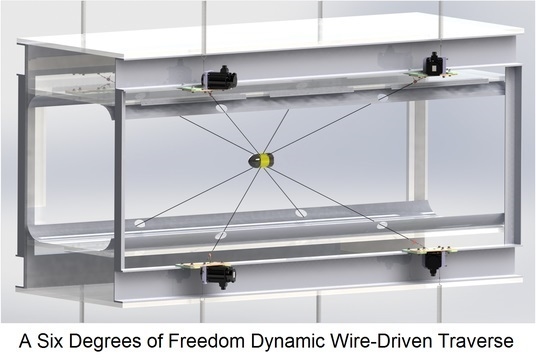
This traverse is designed as an add on to an open-return wind tunnel at Georgia Tech having a test section that measures 91 cm × 91 cm and a maximum speed of 40 m/s, and is also designed such that it can be incorporated and removed from the tunnel, if desired. The support mechanism uses multiple strands of wire rope (aircraft cables) to suspend an aerodynamic platform inside the wind tunnel, and is shown in Figure 1a. The wire ropes have a very small cross-sectional area of 1.13 mm2 and they have low blockage, thus minimizing local acceleration of the airstreams in the vicinity of the model. Theoretically, only six wire ropes would be required for a statically-determinate support of the model. However, the geometry of the wind tunnel and the desire to keep the wire rope and actuators near the corners of the tunnel cross-section led towards an over-constrained support by eight wire ropes. The end of each wire rope is fastened to a servo actuator (YASKAWA SGMAV-10A, having peak torque of 9.55 N·m at a 6000 rpm peak), through a driving pulley. Each servo actuator is mounted outside of the tunnel and dynamically feeds a wire rope inward or outward to alter the position and orientation of the suspended aerodynamic platform. The corner flanges of the wind tunnel are modified to provide eight small openings with enough clearance to accommodate the desired range of wire motion and therefore model motion. It is noted that the motor locations are spaced vertically by 120 cm, horizontally by 128 cm, and streamwise by 176 cm, where these locations are chosen for convenience and can be optimized for future performance objectives, if necessary. All of the driving pulleys have a secondary attachment to an extension spring (with a constant of 208.4 N/m) that provides a preload tension on each wire when the model is in equilibrium (for the current case study, the preload is approximately 60 N). The tension in each mounting wire is measured using an inline miniature load cell (FUTEK FSH00097, with a range of 0–110 N, a non-repeatability of 0.055 N, and a mass of 0.02 kg). The temporal response of the raw load cell signals is on the order of 10 kHz, but these signals are pre-filtered and sampled at a rate of 1 kHz to match the controller rate (see Section 2.4). Figure 1b shows one constructed servo actuator assembly, with labeled components, as all eight servo actuator assemblies are identical.
During the system design phase, several different types of motor actuators were considered for this application. Gear motor actuators could provide more output torque than the direct-drive configuration, but they would have too much inertia to meet the dynamic response goals. All types of linear actuators examined had limitations with response speed or maximum achievable wire rope tension, where the design goals for motion are 50 Hz controlled motions of model deflections of up to 5 mm, and wire tensions of up to 110 N. A vane-type hydraulic rotary actuator would be a compact, high torque, and high response rate solution, but it would require a hydraulic reservoir and pressurization system, and it was deemed less applicable compared to the realized rotary servo actuator shown in Figure 1b, although it would also achieve all of the design goals.
2.2. Motion Capture System
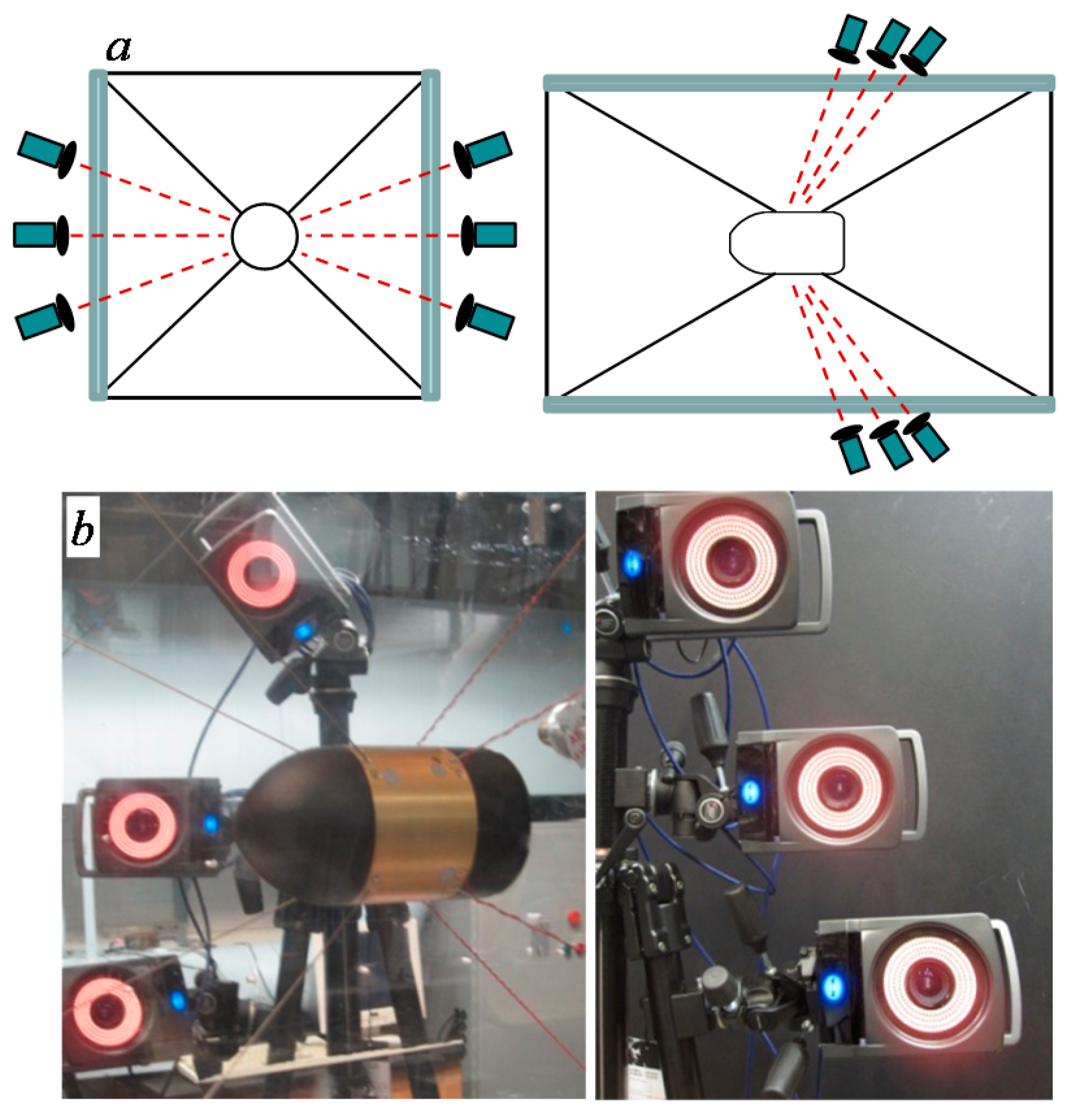
The primary goal of this traverse is to achieve accurate real time motion control of an aerodynamic platform with disturbance rejection. A VICON MX Motion Capture System was acquired for measuring the spatially- and temporally-resolved motion of the wire-mounted model in the wind tunnel (Figure 2). This system consists of: (1) six MX-T40S cameras, each with a 12.5 mm lens (capable of up to 515 fps at full frame, and 2000 fps with a limited view), an electronic freeze frame shutter, and a resolution of 4 megapixels; (2) a MX-Giganet interface of the cameras to a camera host computer (provides power, synchronization, and data transfer); and (3) VICON Tracker 2.0 Software for low latency data streaming to the traverse controller computer.
The cameras are mounted around the wind tunnel’s test section and are focused on the wire-mounted model. The current system utilizes overlapping fields of view to determine the time-resolved (6-DOF) position of the moving model in the wind tunnel at a frequency of 600 Hz. The model’s position is tracked using an optical correlation based on an array of small reflective round markers that are affixed to the model to reflect near infrared (NIR) light that is emitted by diode array built into each camera. The placement of the cameras can be arbitrary as long as the six projected images of these markers measured by the cameras contain enough information to fully define the 6-DOF motion of the model (shown in Figure 2a with both the front and top views of the system). The camera system is calibrated by dynamically moving a calibration target with three reflective markers through the measurement volume. Once the system is calibrated, a static image of a calibration plate of reflective markers is measured to construct a template that is saved on the host computer to transform the marker measurements into the dynamic aerodynamic model coordinates with respect to the wind tunnel frame of reference. An example of the chosen camera locations are shown in Figure 2b. After the system is calibrated, the VICON Tracker software calculates the error in each marker (having typical values between 0.05 and 0.5 mm, dependent on the calibration and camera locations), which are used to calculate the error in the measured model coordinates.
2.3. Case Study: Axisymmetric Model
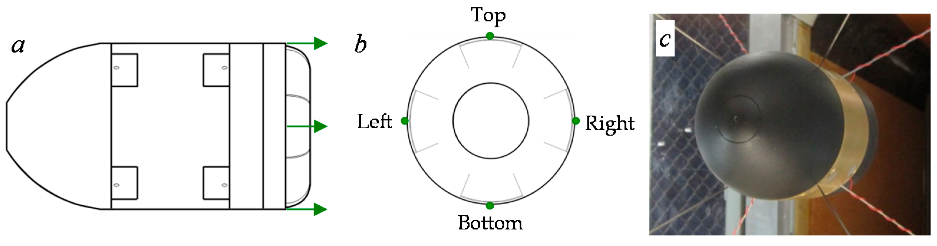
This traversing system is designed to handle a variety of models including munitions, small-scale unmanned aerial vehicles (UAVs), parafoils, parachutes, and rotorcraft configurations. For the purposes of testing of the traverse, the model used as an example case study is an axisymmetric body, as shown in Figure 3, which has been of interest in prior investigations (e.g., [12,13,14]). This axisymmetric wind tunnel model (Figure 3) is assembled using stereo-lithographed (SLA) and aluminum components (D = 90 mm, L = 165 mm, m = 0.53 kg). The mid-section and nose are hollow and connected to the tail section by a central shaft. After assembly, the SLA model surface is painted black resulting in an average surface roughness of approximately 5 μm and then machined flush on a lathe with the central piece. In addition, six reflective circles of 7 mm diameter are attached on the surface for the motion analysis system, and each marker was made from 3M 7610 retroreflective tape of 0.4 mm thickness. These markers are arbitrarily placed so that each camera sees three of them (three of which can also be seen in Figure 2b and Figure 3c).
A secondary requirement for this traverse is that it can provide electrical power to the wind tunnel model to enable future use of flow control applications. In the axisymmetric model example, four independently-driven synthetic jet actuators (labeled the top, left, bottom, and right actuators, as shown in Figure 3b) would be, in principle, integrated and distributed along the perimeter of the tail section, as they would comprise the flow control components in a follow-up study. The electrical power that would be used as a source for the synthetic jets is routed through weaved positive voltage lines (30 AWG) along the mounting wires on the downstream end of the model (shown in Figure 3c), where the entire system is grounded.
The range of translational and rotational motions of the traverse are heavily dependent on the location where each mounting wire is attached to the model (the range of translational motions are also dependent on the locations of the eight servo actuators). For example, if the wires are mounted such that they are equally distributed in the azimuth with 90° between each wire, a roll motion would be impossible, and this scenario is shown in Figure 4a. If the wires are not equally distributed in the azimuth, two symmetric groups of wires can be tightened or loosened to provide roll, as shown in red and green in Figure 4b. The theoretical maximum roll (with full controllability) occurs when one of these symmetric groups becomes in line with the center of the wire mounts, where this limit case is shown in Figure 4c, which occurs if the green set of wires in Figure 4b are tightened. A similar argument can be applied to both the pitch and yaw directions of the model looking at the side of the model or the top of the model, respectively. It is noted that in the front view shown in Figure 4, the projections of the four upstream and four downstream wires overlap, and these respective overlapping wires need to be tightened or loosened equally in order to prevent any pitch or yaw dynamics. The current mounting locations were chosen such that the model can theoretically have a significant and comparable range in all three rotational directions. These realized locations are centered on the model and displaced vertically by ±35.7 mm, horizontally by ±27.4 mm, and streamwise by ±26.3 mm. The extent of the realized traverse motion is discussed in detail in Section 3.1.
2.4. Electrical Traverse Components
The electrical subsystem of this traverse can be considered as being comprised of three separate composite elements. The first element is a “host” computer which is used for implementing the real time traverse controller and has two Quanser Q8 real time data acquisition boards which are used for signal communication of the servo motor command and encoder signals, as well as the flow control actuator commands. The second element is a high power distribution system that routes up to 1 kW power to servo amplifiers for each of the servo motors. Particular attention was given to proper wire routing and grounding in order to minimize electromagnetic interference (EMI) contamination of the measured signals. Each servo motor has an integrated 20 bit differential quadrature absolute encoder, where the output is converted to a single ended signal by custom electronics, and is sampled by the host computer through one of the Q8 boards. The third element is a custom multichannel Ethernet data acquisition (DAQ) system that samples the load cells. The load cell signals are on the order of mV and are susceptible to noise, so each load cell is routed with a short cable to signal conditioning electronics that have an instrumentation amplifier and passive resistor-capacitor (RC) filtering. These signals are then transmitted through universal data protocol (UDP) packets at a nominal frequency of 1 kHz to the host computer.
The user interfaces with a master computer that uses Simulink as an interface to build the controller. Upon completion of the desired controller, Simulink generates a “C” code that is cross compiled into a QNX binary. This binary is copied across an Ethernet network to the host computer (which utilizes a QNX operating system). When the master computer sends the execution command, the controller binary on the host machine is executed in a hard real time environment, which sends time-stamped signals back over Ethernet to the master computer for accurate data recording. The host machine is also connected via Ethernet to the broadcasted signal from the VICON machine to use the position measured from the camera system for feedback to the control system code. It should be noted that the driving signals for flow control can also be generated by the controller and output from the host computer for referencing/triggering of external waveforms and signals.
2.5. Control Systems Design
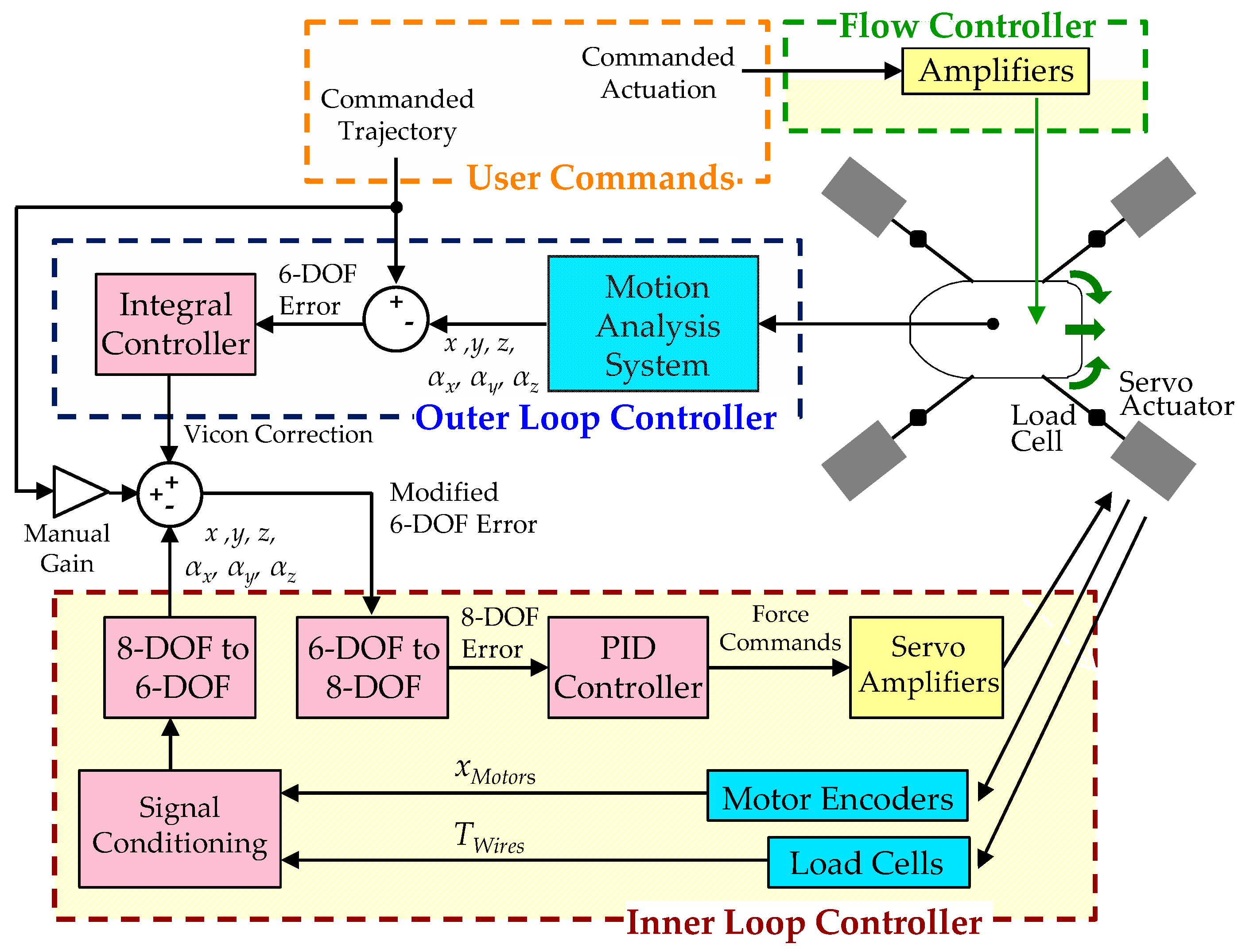
The designed traverse is controlled through the trajectory-tracking controller depicted in Figure 5. First, the user can provide two command inputs; a time trace for the desired model trajectory in 6-DOF, and a time trace for the actuation commands to, for example, amplitude modulate all four synthetic jet carrier waveforms, when flow control needs to be utilized. Second, the 6-DOF commanded motion is converted into eight servo motor commands (6-DOF to 8-DOF), which is calculated through the geometry of the model and chosen mounting points, assuming the wires are incompressible. The command signal to each servo actuator is then generated using eight proportional-integral-derivative (PID) controllers with the same coefficients (κP,inner = 4.24 N·m/rad, κI,inner = 21.20 N·m/(rad·s), (κD,inner = 0.02 N·m·s/rad) which commands the torque in the motors. It is noted that with pure feedback control, there will be a phase lag between the desired command and the realized command, so the motions are currently restricted to time harmonic motions where optimal PID coefficients yield an output that is self-similar to the desired command with a change in phase and amplitude. The realized motion is then calculated through measuring the conditioned encoder signals and inverting these servo motor positions to the model position using a least squares algorithm (8-DOF to 6-DOF). This control loop is considered the “inner loop controller” in Figure 5. It is noted that this inner loop controller is sensitive to errors in the geometric parameters of the traverse (e.g., mounting locations, or damping and friction of the motors). In order to compensate for this geometric model, as well as the change in the amplitude of the desired command, an “outer loop controller” shown in Figure 5 is implemented to adjust the command of the inner loop based on the motion analysis system to allow for accurate trajectory tracking. The outer loop uses an integral error feedback controller that is set such that the measured trajectories reach the desired ones within 10 s (κI,outer = 0.3 s−1 for the 3-DOF translational commands and 0.1 s−1 for the 3-DOF rotational commands). In addition, a manual gain of the inner loop command is implemented, determined by matching the magnitudes of the measured amplitude to the desired amplitude, which is dependent on the frequency and desired motion.
The real time wire tensions measured through the load cells are used to extract the aerodynamic forces and moments on the model. This is realized by using a free body diagram in a control volume (CV) shown in Figure 6, where the aerodynamic forces are calculated by the inertial force, , of the model (acting at the center of gravity, CG, and calculated from its estimated acceleration) with all other forces subtracted. These other forces include the weight of the model (, acting at CG), the tension in the wires, , and the estimated aerodynamic drag of the wires alone, . The latter is calculated assuming the wires are cylinders with pure form drag (CD = 1.25) and no friction drag, using the real time location of both the model and motor wire ends and calculating the normal projection of the flow. It is noted that each wire force is estimated as acting on the midpoint between the tunnel flange and the respective real time location of the wire mount on the model, and acting in the direction normal to the wires. The resultant force is the aerodynamic force on the model, , and a similar approach can be used to determine the moments by weighting each force by the location at which it acts. Measurements of the aerodynamic forces for the axisymmetric body using this force balance are presented in Section 3.2. The current trajectory-tracking controller described in this section restricts the model to a prescribed trajectory, where the model has a negligible response to external aerodynamic forces (where the disturbance force is on the order of ~1 N, and the spring constant of the cables are on the order of ~100,000 N/m). It should be noted, however, that a free flight controller can instead be designed where the model would respond directly to the disturbance forces (by using the load cells as the primary feedback instead of the encoders and camera signals), but a more aggressive controller would have to be implemented in the inner loop to induce dynamics that do not significantly lag the induced forces, and this type of controller is considered for future work.
3. Results
3.1. Motion Response
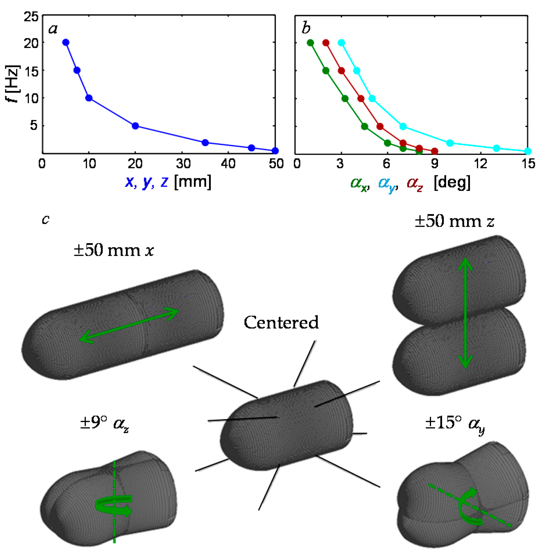
The system dynamic performance is characterized in terms of displacement range and frequency of sinusoidal commands, and is depicted in Figure 7. Although the mounting points of the wires on the motors and the model determine the ideal maximum range of motion with limitless tension and unbreakable wires, this range diminishes for a fixed maximum tension. This range is also frequency dependent and diminishes with higher frequencies as the wires have to support an accelerating model with a larger inertial force. Therefore, the current controller is tested with a range of frequencies and the maximum range of motion in all six degrees of freedom is measured with a maximum wire tension of 110 N, and the results are shown for translations and rotations, in Figure 7a,b, respectively. This frequency response is dependent on all of the aforementioned geometric and controls parameters and can be further optimized by modifying these parameters, if necessary. The measured displacement amplitude that is realized is 50 mm in translation (x, y, and z), and rotations of 8° , 15° , and 9° at a frequency, f = 0.5 Hz, and decreases to 5 mm (x, y, and z), 1° , 3° , and 2° at f = 20 Hz. Four of these motions are visualized in Figure 7c, with streamwise (x) translation, vertical (z) translation, pitch (), and yaw ().
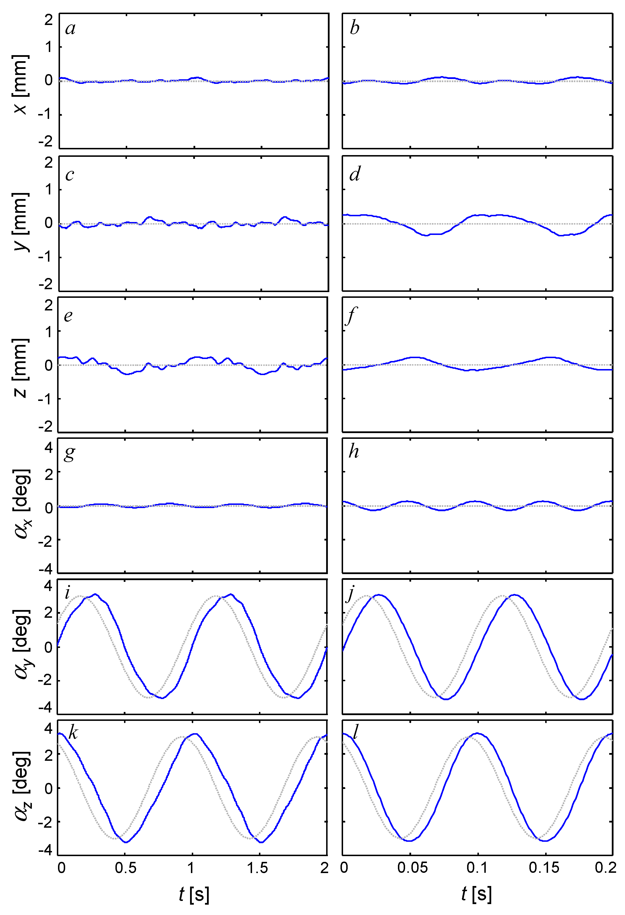
To test the control authority of the traverse for 6-DOF motion tracking, a combination of rotations is commanded (pitch and yaw out of phase) and the instantaneous measurement is shown in Figure 8 with streamwise translation x (Figure 8a,b), cross stream translation y (Figure 8c,d), vertical translation z (Figure 8e,f), roll (Figure 8g,h), pitch (Figure 8i,j), and yaw (Figure 8k,l), respectively. The commanded signal is a 3° amplitude sinusoidal pitch and sinusoidal yaw, 90° out of phase with each other. This same motion is executed with a representative “low” frequency of 1 Hz in Figure 8a,c,e,g,i,k along with a “high” frequency of 10 Hz in Figure 8b,d,f,h,j,l. Both of these motions are executed with wind tunnel flow (ReD = 2.3 × 10⁵) to demonstrate the disturbance rejection of the controller. The time resolved path captured by the motion analysis system is shown in blue while the commanded signal is shown in dotted gray. These data show significant agreement between the commanded and measured signals in terms of peak-peak magnitude (within 5% at 1 Hz in Figure 8i,k and 7% at 10 Hz in Figure 8j,l), with a phase lag of 40° at 1 Hz and 30° at 10 Hz. The realized deviations in the four other degrees of freedom that are not commanded are small: within 0.5° in roll (Figure 8g,h), and within 0.3 mm in all translations (Figure 8a–f). As mentioned in Section 2.2, the errors in the motion measurements for this data set (which is the same as for the motions in Section 3.2 and Section 3.3) are calculated using the motion analysis system calibration error output (0.45 mm per marker on average), yielding errors of 0.18 mm in translation and 0.02° in rotation. It is noted that these instantaneous traces are measured 10 s after the traverse is activated after the transient response of the traverse has settled. The measurements that are shown in Figure 8 can also be used as feedback to the triggering lines for flow diagnostics (e.g., particle image velocimetry (PIV)) and/or flow control, and therefore as long as the flow control is a function of the measured DOF the phase lag between the commanded and measured trajectory is inconsequential for the considered harmonic motions. In this section, the wind speed is fixed at 40 m/s and it is noted that the traverse controller treats the external aerodynamic forces on the model as disturbances to be rejected with PID control. Keeping fixed PID coefficients, the phase lag of the commanded and realized responses would increase with increasing wind speed, as the disturbance force grows, but in the present investigations, the PID parameters are pre-adjusted for a given ReD and can be further tuned with a change in the wind speed.
3.2. Force Response
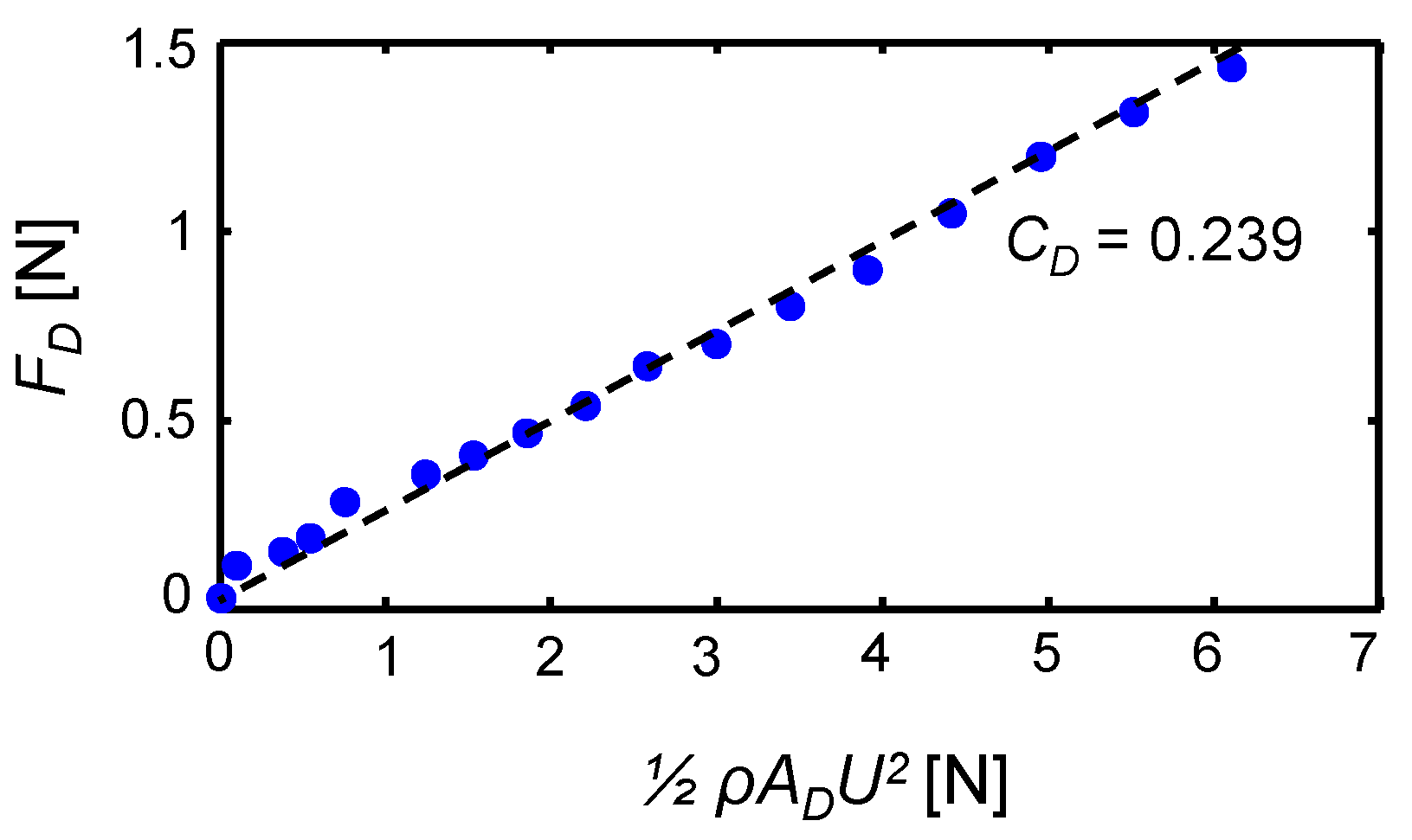
The second analysis that is implemented on the traverse is a validation of the force and moment measurements. Initially, the drag force on the stationary centered model (FD) is measured over a range of wind tunnel speeds, U0, of up to 40 m/s (0 < ReD < 2.3 × 10⁵), and these data are presented in Figure 9a. The measured drag coefficient is CD = 0.239, which is shown in a dotted line, and is in good agreement with the expected drag coefficient of CD = 0.25 (for a similar ogive model with a sharp aft end, see Hoerner [15]). For this stationary centered model, all other forces are nominally zero, and are omitted for brevity. It is noted that for all of the forces presented in this section the force balance method shown in Figure 6 (see Section 2.5) is applied: the combination of the inertial and gravitational forces is measured first from the model executing the prescribed motion command without wind in the tunnel, and the aerodynamic force on each wire is calculated assuming the wires are cylinders with pure form drag (CD = 1.25). The drag on each of these wires is normal to the wire and, in general motion, projects components in all six of the measured forces and moments in the system. For Figure 9, the gravitational force measured (model, wires, and load cells) is a constant, there is no inertial force, and the estimated aerodynamic forces on the wires add up to a pure drag force. These forces are subtracted off of the raw measured forces, which yields the aerodynamic drag force that is used to calculate the model CD. When the model is set in motion, the projected gravitational moment changes with time as the location of the center of gravity varies, and the inertial force and aerodynamic forces on the wires also change with time. All of these time-varying forces are predicted (inertia and gravity effects are estimated from a commensurate measurement without wind) and subtracted from the raw measurement in order to yield the estimated aerodynamic forces. In addition, for the remainder of this paper the aerodynamic moments are measured relative to the center of the model wires at 0.54 L from the nose. It should be also noted that the wires do not only affect aerodynamic measurements, but also present additional sources of vorticity in the flow. However, increased levels of the flow fluctuations behind the wires do not appear to alter the dominant body wake dynamics, and the coupling between the two is deemed insignificant (see Lambert et al. [14]).
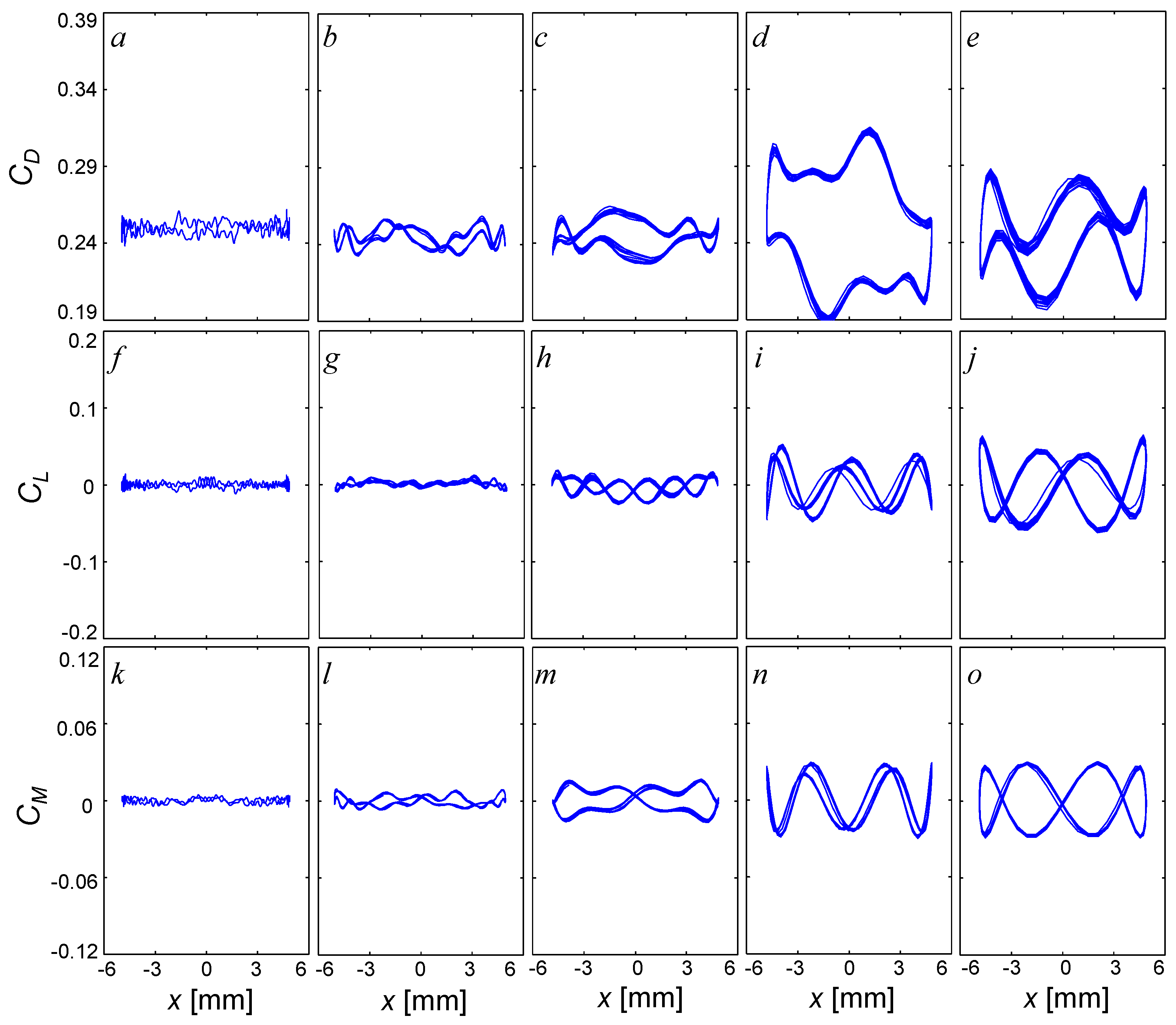
Once the force on a centered stationary model is characterized, three canonical motions are investigated: dynamic pitch, plunge, and streamwise displacement. The first motion presented in Figure 10 is dynamic = ±3° (±0.052 radians) amplitude, simple harmonic pitching. This motion is quantified by the drag and lift force coefficients as well as the pitching moment coefficient , and for the rest of this force investigation, the free stream is set to U0 = 40 m/s (ReD = 2.3 × 10⁵). For these flow conditions, the measured side force and roll and yaw moments are negligible in all three of these canonical motions, and they are omitted for brevity. Figure 10a–e show CD, Figure 10f–j show CL, and Figure 10k–o show CM with the pitching angle, . Figure 10a,f,k show the a quasi-steady response at f = 1 Hz, (or a reduced frequency of = 0.013), and the increased frequency to 5 Hz (k = 0.065, Figure 10b,g,l), 10 Hz (k = 0.130, Figure 10c,h,m), 15 Hz (k = 0.194, Figure 10d,i,n), and 20 Hz (k = 0.259, Figure 10e,j,o). For reference, the values of the CD, CL, and CM for a static model at varying fixed angles of attack with the same geometry [14] are superimposed in Figure 10a,f,k. The baseline CD vs. presented in Figure 10a has a quadratic shape with a minimum of CD = 0.24 at = 0 and a change in magnitude of around 25% (0.24 to 0.3). As frequency is increased, the quadratic functionality in the drag with angle becomes broken and the cycle average drag increases to 0.3 at 15 Hz (Figure 10b–d), and then reduces to 0.28 at 20 Hz (Figure 10e). It is noted that the shedding frequency of this model is expected to be around 100 Hz (StD = fD/U0 was measured to be ~0.2, for a similar axisymmetric body [16]), and the high frequency variations in CD (as well as CL and CM) that are not present in the quasi-steady results are at frequencies of harmonics of the model motion near this shedding frequency. The baseline steady CL vs. presented in Figure 10f is quasi-linear with a slight hysteresis and a lift slope of CL/ ~0.05/°. Upon increasing the pitching frequency to 10 Hz (Figure 10g,h), the hysteresis in the lift coefficient increases while the average lift slope remains similar, and at higher frequencies this slope diminishes to 0.03/° and 0.025/° at 15 and 20 Hz, respectively (see Figure 10i,j). The tendency of the CL (and CM) hysteresis to increase with frequency is attributed to unsteady effects of the flow (the magnitude of the wake’s response time remains roughly similar as the model cycle time decreases). The quasi-steady CM is shown in Figure 10k, with an increasing slope CM/ with frequency from 0.01/° at 1 Hz to 0.025/° at 20 Hz, with a large increase in the hysteresis of the response at higher frequencies (Figure 10l–o). It is noted that this “average slope” is defined as the slope of a linear fit through the dataset and does not take in account variations due to the hysteresis. In addition, having a positive average slope of CM with implies that the model is unstable in pitch (the moment increases with an increase in the pitching angle), as expected.
The second motion investigated is dynamic z = ±5 mm (z/D = ±0.056) amplitude simple harmonic plunging, shown in Figure 11. Figure 11a–e show CD, Figure 11f–j show CL, and Figure 11k–o show CM with the plunging coordinate, z, analogous to Figure 10, with the same flow conditions, frequencies, and timing. As the motion increases in frequency, the time averaged CD stays around the same at 0.24, with the introduction of a higher frequency fluctuation (varying in magnitude from 0.01 to 0.08 in Figure 11a–e) attributed to the wake instability. The quasi-steady CL is approximately invariant (Figure 11f), but has the introduction of a small negative slope at higher frequencies (CL/z = 0.015/° at 10 Hz, 0.01/° at 15 Hz, and 0.015/° at 20 Hz) in addition to a large higher frequency fluctuation (also attributed to shedding). This negative average slope of CL with z implies that the model is stable in plunge, as the aerodynamic force opposes the plunging direction. The quasi-steady CM has slight variations, shown in Figure 11k, with negligible slope throughout its frequency, until the plunging frequency is 20 Hz, with the introduction of a CM/z slope. This may be due to small deviations between the commanded zero pitching angle of the model and the realized pitching angle, as the pitching moment is very sensitive to pitching angle at this large unsteady frequency (compare Figure 10o and Figure 11o).
The third and last canonical motion is dynamic x = ±5 mm (x/L = ±0.030) amplitude simple harmonic streamwise displacement, shown in Figure 12. CD (Figure 12a–e), CL (Figure 12f–j), and CM (Figure 12k–o) are presented with the same frequencies, timing, and conditions as Figure 10 and Figure 11, for completion. For this motion, it is noted that both the motion and the freestream velocity are in the same direction, so the predominant changes occur in CD, while the changes to CL and CM are attributed only to phase locking to the instability in the wake, and are approximately symmetric with zero time averaged values (Figure 12f–o). The time averaged value of the drag retains a value of approximately 0.24, with a growth in hysteresis at 10 Hz (Figure 12c), which maximizes at 15 Hz (Figure 12d), and then decreases at 20 Hz (Figure 12e). It is noted that for most of these drag measurements the average slope of the drag is zero, with the exception of 15 Hz where there is a slight slope of CD/x of −0.01/° which suggests this motion is neutrally stable (the aerodynamic drag is roughly invariant to changes in streamwise coordinate throughout most frequencies). This can be expected as this motion can be analyzed as a fluctuation of the freestream with a value of 2πfx = ±0.0314 to 0.628 m/s, which should not induce large fluctuations in the steady drag coefficient, and the only induced effects are expected to be induced in the unsteady aerodynamics regime.
3.3. Wake Response
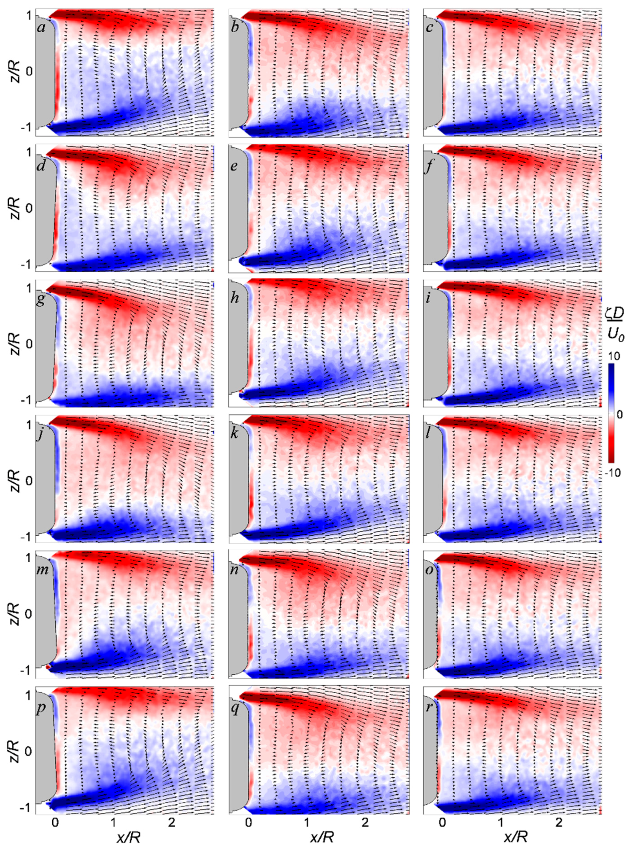
In order to understand the flow mechanisms that result in forces measured on the moving body mounted in this traverse, it is necessary to be able to measure or estimate the wake response around the moving model. The wake response can be measured relative to the real time states of the model as the traverse controller outputs an analog trigger to external devices at either fixed time or fixed trajectory offsets. This triggering system is used to trigger an external LaVision particle image velocimetry (PIV) system to capture instantaneous images of the wake at the aft end of the model in an interrogation region of 1.6D × 1.2D (3.2R × 2.4R) in a vertical region along the centerline of the model. Figure 13 shows six phase-averaged flow fields (each based on 300 individual realizations) for the = ±3° (Figure 13a,d,g,j,m,p), z = ±5 mm (Figure 13b,e,h,k,n,q), and x = ±5 mm (Figure 13c,f,i,l,o,r), with velocity field vectors overlaid on a raster plot of the cross-stream vorticity, ζ, at ReD = 2.3 × 10⁵ (U0 = 40 m/s). The frequency of these motions are chosen to represent unsteady wake dynamics at 20 Hz (τ = 0.05 s), and the phases shown are equally spaced in time, t, throughout the cycles at: t/τ = 0 (Figure 13a–c), 0.167 (Figure 13d–f), 0.333 (Figure 13g–i), 0.500 (Figure 13j–l), 0.667 (Figure 13m–o), and 0.833 (Figure 13p–r). For reference, the aft end of the model is superimposed on this data and shown in gray. The wake behind this model has three primary regions of interest: (i) the shear layer with the largest vorticity concentration; (ii) the inner wake with a reversed flow and smaller concentration of vorticity, which is bound by the wake stagnation point; and (iii) the boundary layer along the aft end of the body, which clearly indicates the time-resolved stagnation point on the body. For = ±3° pitch (Figure 13a,d,g,j,m,p), the chosen time scale leads to an unsteady flow response, where the wake development time scale is on the same order of the model motion. This leads to the wake response being out of phase with the model (note the wake is approximately centered between Figure 13a,d, and Figure 13j,m, respectively, implying an approximate phase lag of the wake response of about 30°) which is also commensurate with the hysteresis measured previously in CL vs. and CM vs. (Figure 10e,j,o). For z = ±5 mm plunge (Figure 13b,e,h,k,n,q), the wake response looks similar to pitching with a smaller deflection and a different phase lag (an easy way to observe this effect is to compare the development of the stagnation point on the model in Figure 13b,e,h,k,n,q to Figure 13a,d,g,j,m,p). For x = ±5 mm streamwise displacement (Figure 13c,f,i,l,o,r), the wake seems approximately unchanged and translates with the model with an addition of small fluctuations in the vorticity in the reversed flow region of the inner wake. In addition to Figure 13, videos are provided with the manuscript that depict the = ±3° pitch (Video S1), z = ±5 mm plunge (Video S2), and x = ±5 mm streamwise displacement (Video S3) wake dynamics at f = 20 Hz (see Supplementary Materials). These results show that the present dynamic traverse is capable of effecting high frequency harmonic motions of the attached model, as well as resolving both the induced aerodynamic forces on a model and the corresponding wake response.
4. Discussion and Concluding Remarks
The present experimental work is focused on a design, manufacturing, and implementation of a novel 6-DOF traversing mechanism that enables realization of dynamic states of a model and characterization of its motion and force/moment responses. This traversing mechanism suspends a wind-tunnel model by eight wires with custom servo actuators. This mechanism is designed to move all the wires in patterns that can cause rotation in three independent axes: roll (8°), pitch (15°), and yaw (9°), as well as the respective independent translations: streamwise, cross-stream, and vertical; all within a range of 50 mm at lower frequencies. The range of the traverse is dependent on the frequency of motions as well as the geometry of the model which is to be investigated. Each wire has an incorporated load cell that resolves the tension, and thereby captures the aerodynamic forces and moments on the model. Motion is executed by an in-house real-time controller that provides signals to the servo actuators as commanded. The executed motion is recorded in six degrees of freedom by an external VICON camera system (600 fps), which output is fed into the controller as a feedback signal to maximize the accuracy of motion. The real-time control system utilizes two Quanser data acquisition boards.
The traverse-driven model motion is tested in multiple degrees of freedom, and it could generate desired complex trajectories, comprised of the combined translational and rotational motions. These trajectories could be realized with minimal error compared to the commanded motion, being executed in a PID control loop in addition to having feedback from the motion analysis system. In the present work, a time trace of pitch and yaw commands out of phase are generated to demonstrate the robustness of this traverse controller in multiple degree of freedom motion at a representative “low” frequency of 1 Hz, and a representative “high” frequency of 10 Hz.
For the purposes of the traverse testing, an axisymmetric model is used as a case study. Three canonical motions of this model are chosen for investigating both the aerodynamic loads as well as the commensurate wake responses behind the model: sinusoidal pitch at ±3°, vertical plunge at ±5 mm, and horizontal displacement at ±5 mm. The corresponding measurements were taken at multiple motion cycle frequencies ranging from 1 to 20 Hz. Several known characteristics of this platform were used to validate the force measurements, such as its drag coefficient, its static values of drag, lift, and moment at fixed angles of attack, and its stability. The induced aerodynamic moment on the body undergoing pitching motion is of the same sense as the pitch angle, and is unstable. In contrast, the lift induced force on the body undergoing vertical plunge is of the opposite sense and is stable. It is also shown that the higher frequency motions excite force responses with frequencies that are of the order of the expected vortex shedding frequency of the model geometry. The ensuing wake responses are measured and analyzed, using a triggering system incorporated into the traverse trajectory controller and an external PIV system that resolved the wake development with a cycle frequency of 20 Hz. The test results imply that the developed support mechanism can be used for dynamic tests of various models, with time-resolved trajectory (and its derivatives), aerodynamic loads, and the flow dynamics.
Supplementary Materials
The following are available online at https://www.mdpi.com/2226-4310/3/2/11/s1, Video S1: f = 20 Hz, 3° pitch at U0 = 40 m/s; Video S2: f = 20 Hz, 5 mm, plunge at U0 = 40 m/s; and Video S3: f = 20 Hz, 5 mm, streamwise displacement at U0 = 40 m/s. All videos are at 1/40 real time (6 frames per second with 12 phases per cycle).
Acknowledgments
This work has been supported by Georgia Tech and the Army Research Office.
Author Contributions
Thomas J. Lambert, Bojan Vukasinovic, and Ari Glezer contributed equally to this work, including conception, design, experiments, data analysis, interpretation, and writing.
Conflicts of Interest
The authors declare no conflict of interest.
Abbreviations
The following abbreviations are used in this manuscript:
| DOF | degrees of freedom |
| PIV | particle image velocimetry |
| CAD | computer-aided design |
| NIR | near infrared |
| UAV | unmanned aerial vehicles |
| SLA | stereo-lithography |
| AWG | American wire gauge |
| EMI | electromagnetic interference |
| DAQ | data acquisition |
| UDP | universal data protocol |
| PID | proportional-integral-derivative |
| CV | control volume |
| CG | center of gravity |
References
- Higuchi, H.; van Langen, P.; Sawada, H.; Tinney, C.E. Axial flow over a blunt circular cylinder with and without shear layer reattachment. J. Fluids Struct. 2006, 22, 949–959. [Google Scholar] [CrossRef]
- Higuchi, H.; Sawada, H.; Kato, H. Sting-free measurements on a magnetically supported right circular cylinder aligned with the free stream. J. Fluid Mech. 2008, 596, 49–72. [Google Scholar] [CrossRef]
- Achenbach, E. Experiments on the flow past spheres at very high Reynolds numbers. J. Fluid Mech. 1972, 54, 565–575. [Google Scholar] [CrossRef]
- Taylor, G.S.; Gursul, I.; Greenwell, D.I. Investigation of support interference in high-angle-of-attack testing. J. Aircr. 2003, 40, 143–152. [Google Scholar] [CrossRef]
- Taylor, G.S.; Gursul, I. Support Interference for a Maneuvering Delta Wing. J. Aircr. 2005, 42, 1504–1515. [Google Scholar] [CrossRef]
- Griffin, S.A.; Crooks, R.S.; Mole, P.J. Vane Support System (VSS) A New Generation Wind Tunnel Model Support System. In Proceedings of the 29th Aerospace Sciences Meeting, Reno, NV, USA, 7–10 January 1991.
- Pattinson, J.; Lowenberg, M.H.; Goman, M.G. Multi-degree-of-freedom wind-tunnel maneuver rig for dynamic simulation and aerodynamic model identification. J. Aircr. 2012, 50, 551–566. [Google Scholar] [CrossRef]
- Tuttle, M.H.; Gloss, B.B. Support Interference of Wind Tunnel Models: A Selective Annotated Bibliography; NASA-TM-81909-SUPPL; NASA Langley Research Center: Hampton, VA, USA, 1 March 1981. [Google Scholar]
- Bacon, D.L. Model Supports and Their Effects on the Results of Wind Tunnel Tests; NACA Technical Notes 130; National Advisory Committee for Aeronautics: Hampton, VA, USA, 1 February 1923. [Google Scholar]
- Ericsson, L.E.; Reding, J.P. Review of support interference in dynamic tests. AIAA J. 1983, 21, 1652–1666. [Google Scholar] [CrossRef]
- Beyers, M.E. Unsteady wind-tunnel interference in aircraft dynamic experiments. J. Aircr. 1992, 29, 1122–1129. [Google Scholar] [CrossRef]
- Abramson, P.; Vukasinovic, B.; Glezer, A. Direct measurements of controlled aerodynamic forces on a wire-suspended axisymmetric body. Exp. Fluids 2011, 50, 1711–1725. [Google Scholar] [CrossRef]
- Abramson, P.; Vukasinovic, B.; Glezer, A. Fluidic control of aerodynamic forces on a bluff body of revolution. AIAA J. 2012, 50, 832–843. [Google Scholar] [CrossRef]
- Lambert, T.J.; Vukasinovic, B.; Glezer, A. Active decoupling of the axisymmetric body wake response to a pitching motion. J. Fluids Struct. 2015, 59, 129–145. [Google Scholar] [CrossRef]
- Hoerner, S.F. Fluid Dynamic Drag, 3rd ed.; Hoerner Fluid Dynamics: Bricktown, NJ, USA, 1965. [Google Scholar]
- Rigas, G.; Oxlade, A.R.; Morgans, A.S.; Morrison, J.F. Low-dimensional dynamics of a turbulent axisymmetric wake. JFM Rapids 2014, 755, R5. [Google Scholar] [CrossRef]
Figure 1.
Computer-aided design (CAD) model of the 6-DOF (six degrees of freedom) traverse (a); and a model of a servo motor assembly (b).
Figure 1.
Computer-aided design (CAD) model of the 6-DOF (six degrees of freedom) traverse (a); and a model of a servo motor assembly (b).
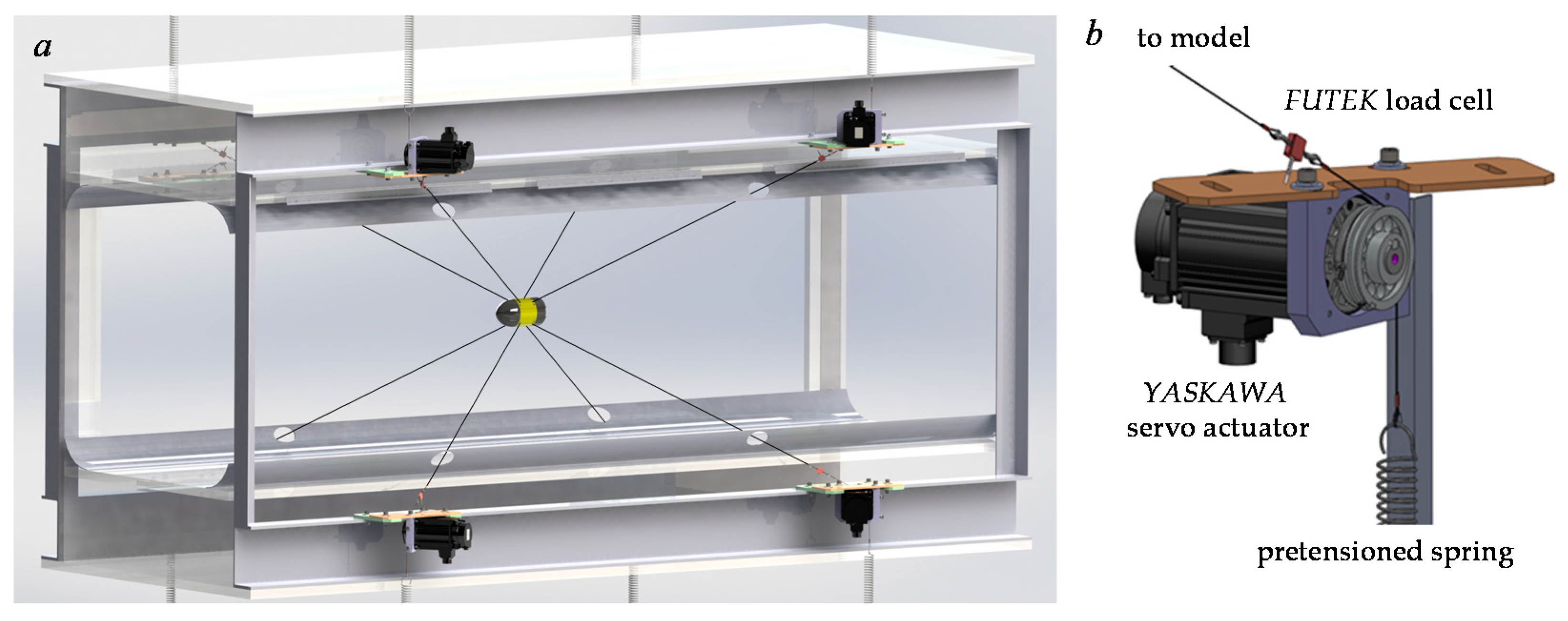
Figure 2.
Schematics (a) and images (b) of the motion analysis system camera orientation.

Figure 3.
Side (a) and upstream (b) views of the CAD wind tunnel model with four hybrid fluidic actuators marked in green, and the model supported by the traverse (c).
Figure 3.
Side (a) and upstream (b) views of the CAD wind tunnel model with four hybrid fluidic actuators marked in green, and the model supported by the traverse (c).

Figure 4.
Orientation of the support where pure roll is disabled (a) and enabled for clockwise roll (green arrows) and counter-clockwise roll (red arrows) (b); along with its respective maximum clockwise roll deflection (c).
Figure 4.
Orientation of the support where pure roll is disabled (a) and enabled for clockwise roll (green arrows) and counter-clockwise roll (red arrows) (b); along with its respective maximum clockwise roll deflection (c).

Figure 5.
Schematics of the traverse trajectory-tracking controller.

Figure 6.
Free-body diagram of the aerodynamic platform and the support wires with the aerodynamic model (blue), inertia (green), gravitational (cyan), and aerodynamic wire (orange) forces, and the wire tensions (red).
Figure 6.
Free-body diagram of the aerodynamic platform and the support wires with the aerodynamic model (blue), inertia (green), gravitational (cyan), and aerodynamic wire (orange) forces, and the wire tensions (red).
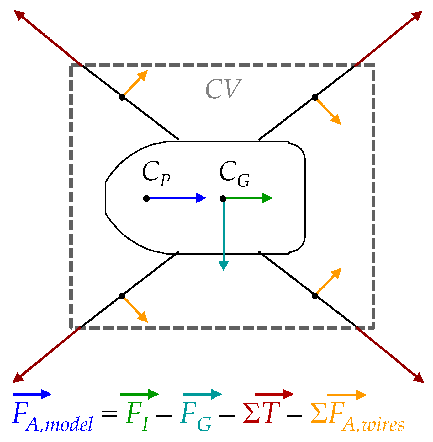
Figure 7.
Frequency response of tested translational (a), and rotational (b) motions, with an illustration of the maximum traverse displacements achieved in four of the degrees of freedom (c).
Figure 7.
Frequency response of tested translational (a), and rotational (b) motions, with an illustration of the maximum traverse displacements achieved in four of the degrees of freedom (c).

Figure 8.
Traverse motion response for 3° amplitude pitch and yaw rotation, 90° out of phase, with measured translation in x (a,b), y (c,d), and z (e,f), and rotations in roll (g,h), pitch (i,j), and yaw (k,l), for frequencies of 1 Hz (a,c,e,g,i,k) and 10 Hz (b,d,f,h,j,l), with a flow ReD = 2.3 × 10⁵. The commanded and measured responses are shown in dotted gray and blue, respectively.

Figure 9.
Measured axisymmetric model drag with varying wind tunnel speed.

Figure 10.
Drag (a–e), Lift (f–j), and Pitch (k–o) coefficients with pitching angle for the axisymmetric model with simple harmonic pitching at an amplitude of αy = ±3° and oscillation frequencies of 1 Hz (a,f,k), 5 Hz (b,g,l), 10 Hz (c,h,m), 15 Hz (d,i,n), and 20 Hz (e,j,o) over a time interval of 1 s, using 100 phase averages, with a flow ReD = 2.3 × 10⁵. The drag, lift, and pitch coefficients measured on the same model geometry at static angles by Lambert et al. [14] are shown in green symbols.

Figure 11.
Drag (a–e), Lift (f–j), and Pitch (k–o) coefficients with simple harmonic plunge at frequencies of 1 Hz (a,f,k), 5 Hz (b,g,l), 10 Hz (c,h,m), 15 Hz (d,i,n), and 20 Hz (e,j,o) and an amplitude of z = ±5 mm, for the same conditions as in Figure 10.
Figure 11.
Drag (a–e), Lift (f–j), and Pitch (k–o) coefficients with simple harmonic plunge at frequencies of 1 Hz (a,f,k), 5 Hz (b,g,l), 10 Hz (c,h,m), 15 Hz (d,i,n), and 20 Hz (e,j,o) and an amplitude of z = ±5 mm, for the same conditions as in Figure 10.
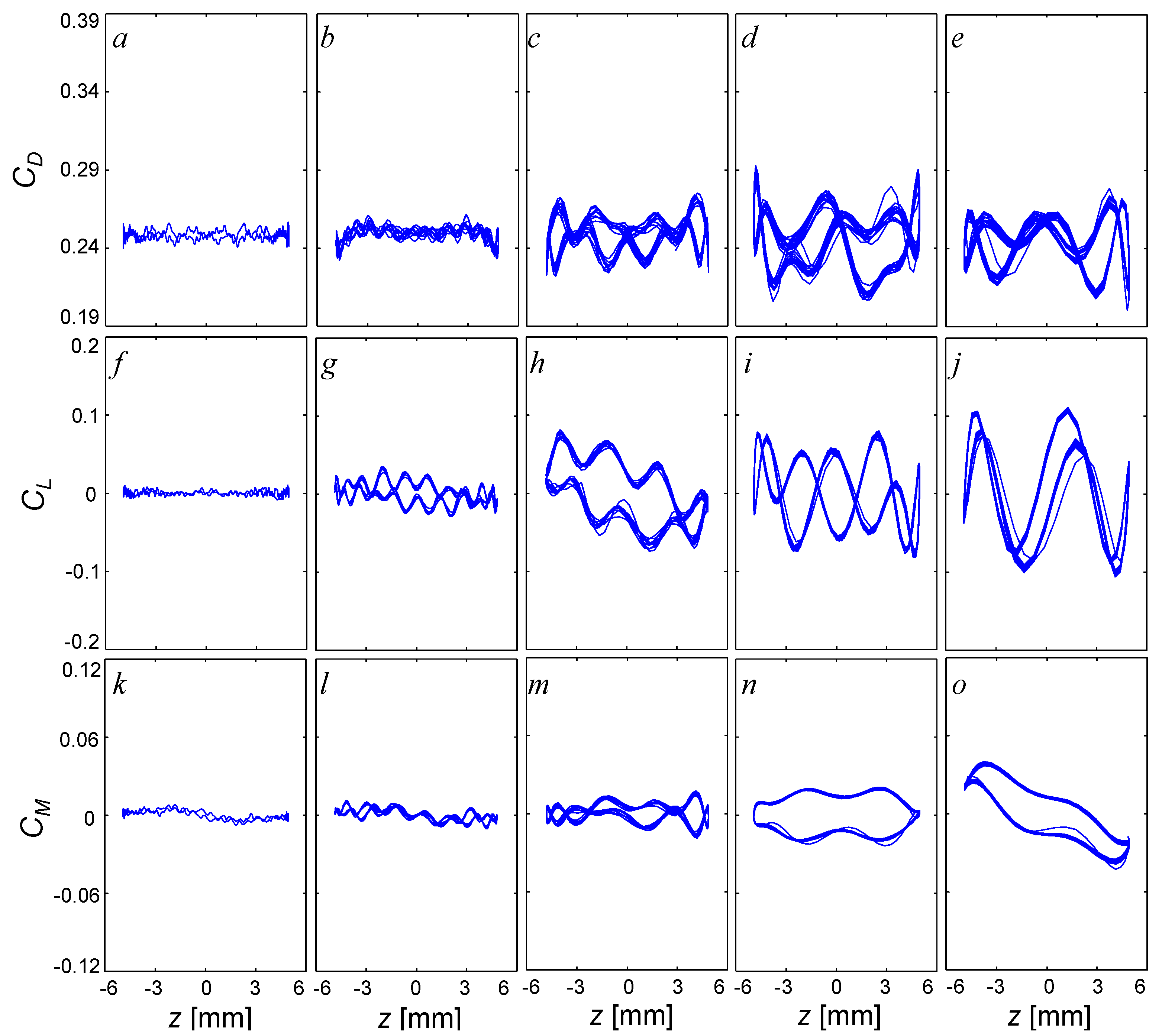
Figure 12.
Drag (a–e), Lift (f–j), and Pitch (k–o) coefficients with simple harmonic streamwise displacement at frequencies of 1 Hz (a,f,k), 5 Hz (b,g,l), 10 Hz (c,h,m), 15 Hz (d,i,n), and 20 Hz (e,j,o) and an amplitude of x = ±5 mm, for the same conditions as in Figure 10.
Figure 12.
Drag (a–e), Lift (f–j), and Pitch (k–o) coefficients with simple harmonic streamwise displacement at frequencies of 1 Hz (a,f,k), 5 Hz (b,g,l), 10 Hz (c,h,m), 15 Hz (d,i,n), and 20 Hz (e,j,o) and an amplitude of x = ±5 mm, for the same conditions as in Figure 10.

Figure 13.
Raster plots of the phase-averaged vorticity field with overlaid phase-averaged velocity vectors for simple harmonic motions (f = 20 Hz) in αy = ±3° pitch (a,d,g,j,m,p), z = ±5 mm plunge (b,e,h,k,n,q), and x = ±5 mm streamwise displacement (c,f,i,l,o,r), at phases t/τ = 0 (a–c), 0.167 (d–f), 0.333 (g–i), 0.500 (j–l), 0.667 (m–o), and 0.833(p–r) with a flow ReD = 2.3 × 10⁵.

© 2016 by the authors; licensee MDPI, Basel, Switzerland. This article is an open access article distributed under the terms and conditions of the Creative Commons by Attribution (CC-BY) license (http://creativecommons.org/licenses/by/4.0/).
Share and Cite
MDPI and ACS Style
Lambert, T.J.; Vukasinovic, B.; Glezer, A. A Six Degrees of Freedom Dynamic Wire-Driven Traverse. Aerospace 2016, 3, 11. https://doi.org/10.3390/aerospace3020011
AMA Style
Lambert TJ, Vukasinovic B, Glezer A. A Six Degrees of Freedom Dynamic Wire-Driven Traverse. Aerospace. 2016; 3(2):11. https://doi.org/10.3390/aerospace3020011
Chicago/Turabian StyleLambert, Thomas J., Bojan Vukasinovic, and Ari Glezer. 2016. "A Six Degrees of Freedom Dynamic Wire-Driven Traverse" Aerospace 3, no. 2: 11. https://doi.org/10.3390/aerospace3020011
Note that from the first issue of 2016, this journal uses article numbers instead of page numbers. See further details here.