1. Introduction
Laminates and sandwiches are used as primary structural components in aerospace and other branches of engineering, owing to their excellent properties (e.g., high specific stiffness and strength, favourable thermo-mechanical properties). In addition, they offer the possibility of optimizing their design by properly choosing the fibre orientation and the stacking lay-up. As an example of ply angle optimization studies and of sandwich optimization, the works of Akbulut and Sonmez [
1] and Khandan
et al. [
2] are cited. Generally, finite-element or closed-form analytic approaches are employed to evaluate objective functions and constraints, while in order to improve efficiency, the solution of the optimal lamination problem is carried out using gradient-based search techniques (see, e.g., Uys and Sankar [
3]) or genetic algorithms (see, e.g., Krishnapillai and Jones [
4]). Customarily, smeared laminate models are employed to compute the structural response, since more realistic models may require much greater computational effort that may be unaffordable for the optimization process. As a consequence, the layerwise effects are usually disregarded, but nevertheless they are a serious design concern. In fact, these effects are responsible for warping, shearing and straining deformations of the normal and out-of-plane stresses consequent to elastic moduli and strengths in the in-plane direction that are much bigger than those in the thickness direction. As mistaken prediction of layerwise effects produces inaccurate evaluations of strength, stiffness, failure behaviour and service life of composites, the structural models should accurately describe the abovementioned effects.
In order to limit the computational effort required, optimization is customarily carried out considering the fibre orientation angle constant throughout the plies and assuming the core properties to be uniform across the thickness. However, with this method, an excellent opportunity for improving performance, damage tolerance and service life is lost. In fact, applications of variable stiffness composites in which the fibres follow curvilinear paths have shown that buckling and first-ply failure loads could be improved, (Sousa
et al. [
5] and Nik
et al. [
6]), stiffness could be maximized, (Pedersen [
7] and Setoodeh
et al. [
8]) and the fundamental frequency could be increased, (Honda
et al. [
9], Narita and Hodgkinson [
10] and Abdalla
et al. [
11]). Moreover, as shown by Jung [
12] and Lakes [
13], structural-hierarchy-guided combinations of materials with different stiffness/dissipation properties allow desired structural properties to be obtained that represent contrasting requirements for uniform stiffness composites, e.g., a larger damping without any stiffness loss.
Manufacturing technologies such as automated fibre placement (Barth [
14], Enders and Hopkins [
15]) and functionally graded materials (FGM) (see, e.g., Mahfuz
et al. [
16]) have paved the way for the spread of variable stiffness composites. Regrettably, the possibility of varying the strength and stiffness properties at each point comes at the cost of a significant growth in the number of design variables in the optimization process. This makes the use of traditional optimization techniques based on gradient search or genetic algorithms impractical, since the computational effort may become too high for structures of industrial interest.
The tailoring optimization technique based on variable-stiffness concepts (OPTI), developed and progressively refined by the authors in references [
17,
18] overcomes this problem since it determines the optimal fibre angle variation over the faces, solving in exact or numerical form the Euler–Lagrange equations following from the extremization of the strain energy under spatial variation of the stiffness properties. The purpose of this technique is to obtain a closed form solution that defines in a specific ply the solution that minimizes the transverse shear stresses at the critical interfaces and the bending deformation. However, any other strategy of interest could be applied making minimal or maximal the strain energy contributions of interest, then solving simultaneously the resulting equations to give the optimal distribution of stiffness properties.
It can be noted that the search for the optimal orientation of fibre paths is carried apart from the computation of the structural response and done one at a time. Therefore, layerwise structural models that are impractical if used with the available optimization techniques, requiring an extremely high computational effort, can be considered under the present approach, in order to give more realistic predictions.
After computation of the optimal fibre distributions through OPTI, the optimization problem of variable-stiffness composites turns into a simple problem of finding the appropriate stacking sequence, like with straight-fibre composites, which can be efficiently solved using the classical optimization techniques.
In order to enable OPTI to provide reliable results, the strain energy of the structure (see [
18]) should be accurately described; accordingly, the present study is carried out employing the multi-layered 3D zig-zag model developed in [
19]. Summing up, this model, which is based on a hierarchic representation of displacements across the thickness, assumes as functional degrees of freedom (d.o.f.) just the classical mid-plane displacements and the shear rotations. These features allow the model to adapt to the variation of solution across the thickness, thus giving very accurate predictions of the piecewise variation of displacements across the thickness and of out-of-plane stress distributions directly from constitutive equations, even for problems with different length and elastic scales. In particular, the through-the-thickness variation of the transverse displacement and of the transverse normal stress, which can have a significant bearing for keeping equilibrium in many practical cases (e.g., thermo-elasticity, cut-outs, free edges, crushing behaviour of sandwiches), are accurately described.
This enables the model to very accurately represent the strain energy stored in the structure, making it suitable for the optimization technique adopted here. It is also suitable for carrying out the analysis of optimized configurations, being as accurate as the high-order layerwise plate models extensively employed to date, but requiring a much lower computational effort, having less d.o.f. In fact, the memory storage dimension and processing time are not considerably larger than those required by equivalent single-layer models.
The numerical results will show that the application of OPTI enables us to obtain fibre distributions compatible with the current manufacturing techniques and leads to a significant improvement of structural performance, in particular a recovery of critical stresses and a reduction of the transverse displacement both for static and dynamic cases.
It will be shown that the application of different distributions computed by OPTI in different zones of the same ply will lead to a reduction in both the shear stress at the critical interfaces of sandwiches and the transverse displacement.
2. The Structural Model and the Optimization Process
The main steps for deriving the structural model and the optimization process are reviewed below.
2.1. Structural Model
In order to accurately and efficiently predict displacements and stresses in laminates and sandwiches, a piecewise variation of the displacements fields is constructed [
19] that
a priori satisfy the stress boundary conditions and the continuity of out-of-plane stresses and of the transverse normal stress gradient at the material interfaces across the thickness. It employs as functional d.o.f. only the displacements and the shear rotations at the middle reference plane. However, it offers the possibility of changing the representation from point to point across the thickness, in order to adapt to the variation of solutions.
The following piecewise representation of the displacements is postulated across the thickness:
The three contributions Δ°, Δi and Δc have the expressions reported hereafter, which are all expressed as functions of the d.o.f. , , , , and of their spatial derivatives.
The contribution Δ
° repeats the kinematics of the FSDPT model:
Having been used in so many applications in the literature [
17,
18,
19,
20,
21,
22,
23,
24,
25,
26,
27,
28], this part does not need further explanation.
The terms Δ
i are postulated to vary piecewise across the thickness, as follows:
The purpose of these contributions is to allow for a change of the representation across the thickness, thus having the appropriate expansion order at any point that can accurately capture stresses from constitutive equations.
The unknown coefficients in Equations (3)–(5) are determined by enforcing the boundary conditions for the transverse shear stresses, transverse normal stress and its gradient at the upper and lower bounding surfaces:
Also, the equilibrium condition is imposed at discrete points across the thickness:
This condition should be imposed in a number of points
np =
Nlay × ord_u − 2,
Nlay being the number of computational layers and ord_u being the order of the expansion across the thickness chosen for the in-plane displacements. The position of the n
p points is chosen arbitrarily, being sure not to consider points excessively near to the interfaces, in order to avoid numerical problems (
i.e., singular or badly scaled matrix). As opposed to previous applications of the model, here, the equilibrium condition Equation (10) is imposed also at the points where fibre orientations suddenly vary as for the optimized plies of
Figure 1, in order to recover the in-plane continuity of the stresses at those points. In details, by integrating along
x it is possible to obtain a continuous (i) σ
xx from Equation (10a); (ii) σ
xy from Equation (10b); (iii) σ
xz from Equation (10c).
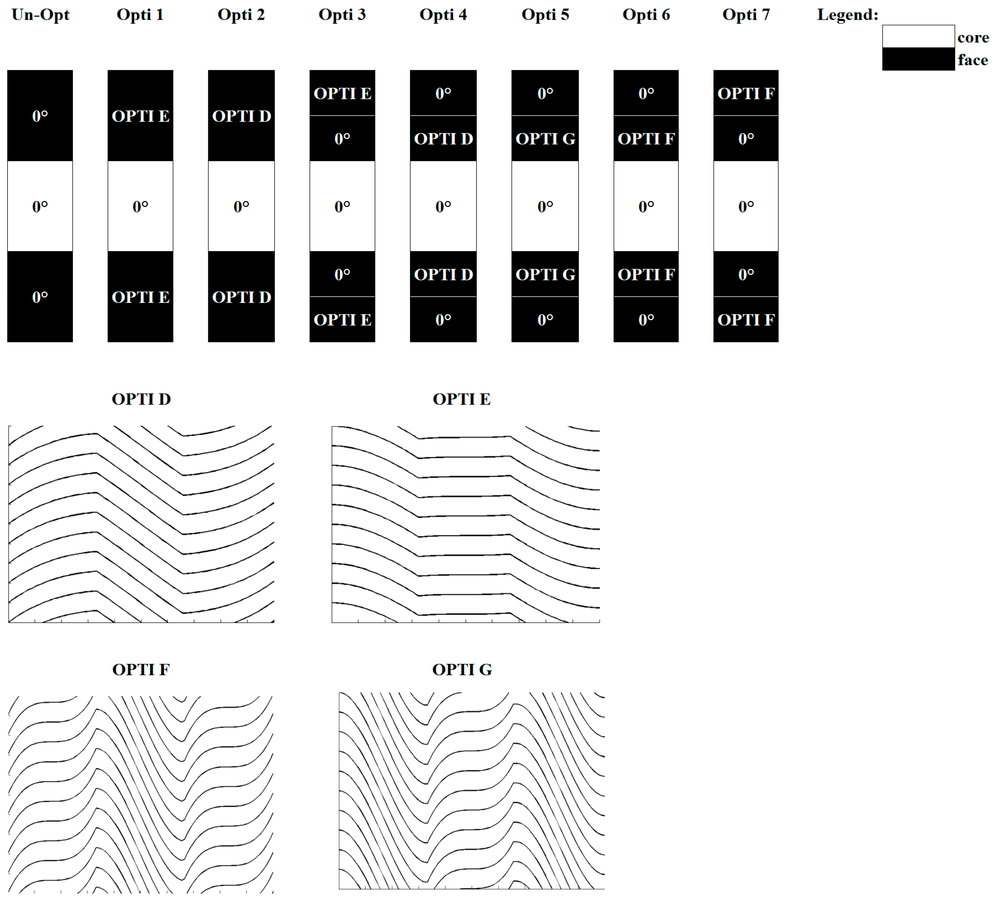
Figure 1.
Lay-ups considered for the local optimization of a sandwich beam.
Figure 1.
Lay-ups considered for the local optimization of a sandwich beam.
The expressions of the piecewise terms Δ
c are chosen as follows:
The Heaviside unit step function Hk makes the contribution of , , , , , , active, since their pertinent interface, i.e., Hk = 1 for and 0 for .
These terms, which should be computed once for any lay-up, are aimed at
a priori fulfilling the continuity constraints at the material interfaces in the thickness direction:
By enforcing these constraints, the displacements
are made C°
continuous at the interfaces of physical and computational layers, with
appropriate discontinuous derivatives across the thickness.
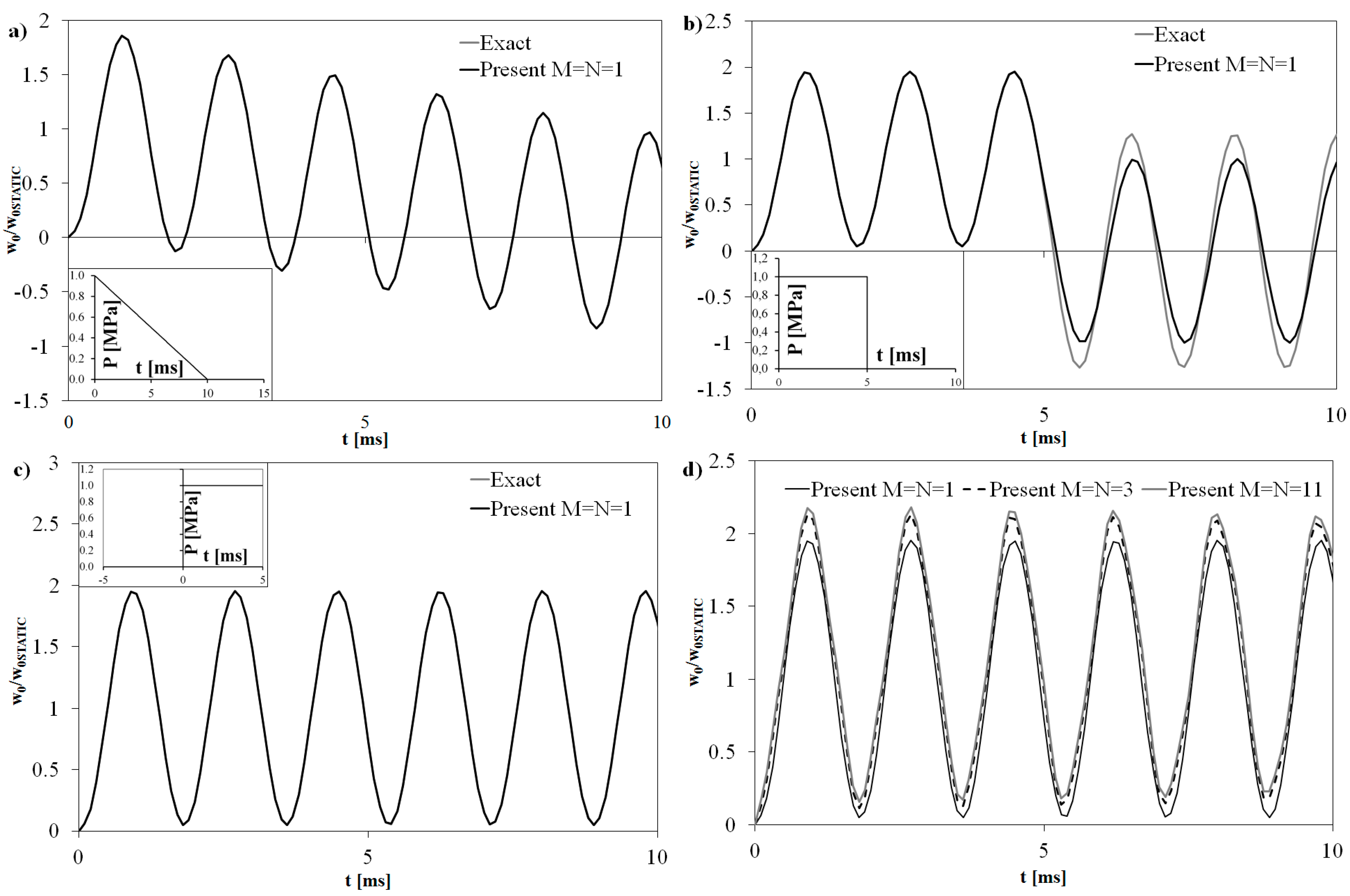
Thanks to this representation, the model is able to obtain results as accurate as those of exact 3D solutions both for static (see [
18,
19]) and dynamic (see
Section 3) analyses. All the unknowns of the model are computed apart one at a time using symbolic calculus, thus consistently reducing the computational effort with respect to the previous models of references [
21,
25] with similar features.
Summing up, as a result, of its features the model provides the following:
- (i)
A correct stress prediction directly from constitutive equations, without using post-processing techniques, such as the integration of local equilibrium equations. In this context, note that such post-processing techniques can fail in capturing accurate interlaminar stresses, as shown by Cho
et al. [
20], and even when they are accurate they are unsuitable as they increase the computational costs;
- (ii)
An improved representation of the strain energy of the structure, which enables a more realistic evaluation of the dynamic response. In addition, a correct description of the strain energy enables a more effective application of OPTI, as shown in [
18];
- (iii)
An improved efficiency (elapsed times reduced at 1/20 with respect to [
21]) obtained through the use of a symbolic calculus tool, because many algebraic computations are carried out separately, one at a time, as shown in [
19]. Since all the unknown coefficients of the model are related to the basic variables through differential equations, it seems that this approach involves an increase of the computational time and the introduction of derivatives of the d.o.f., which are unsuited for developing finite elements based on this model. The former drawback is solved by the workaround of computing these coefficients separately, in closed form as a function of the d.o.f. using symbolic calculus. As mentioned above, this dramatically reduces the computational times. Concerning the derivatives of the d.o.f., they do not represent a problem for the analytical approach adopted here, while they can be avoided in finite elements using techniques such those proposed by Zhen and Wanji [
22] and Sahoo and Singh [
23]. These techniques could determine an increase of the nodal d.o.f., but this latter drawback can be overcome by adopting the technique of [
24];
- (iv)
A low computational effort, which makes this model particularly suited for dynamic and impact analyses that require a great number of iterations in order to calculate the structural response.
2.2. Optimization Technique
The technique used here is based on the idea of finding optimized paths of fibre as solutions to the Euler–Lagrange equations obtained by enforcing the contemporaneous minimization of strain energy contributions of interests (the bending and transverse shear energy) under variation of the stiffness properties. The present technique can be seen as a non-classical optimization technique in which the design variables to be modified are the stiffness properties (through spatial variation of the ply angles and/or of fibre volume fraction and constituent materials) and the constraints are represented by imposition of constant thickness of individual layers, constant overall properties (e.g., averaged stiffness of the “optimized” layers equal to the stiffness of classical layers made of the same constituent materials), the thermodynamic constraints for energy conservation and the Lempriere, Lekhnitskii and Chentsov’s conditions. The objective function is to find a proper distribution of the stiffness properties that minimizes the energy absorbed through unwanted modes (e.g., modes involving interlaminar strengths) and maximizes that absorbed by desired modes (e.g., modes involving membrane strengths). Accordingly, the transverse shear stress concentrations are recovered, while membrane non-critical stresses could be slightly increased. As a consequence, the present technique transfers energy from bending and shear modes to membrane ones through a suited distribution of stiffness properties. The increase of the in-plane contributions to the strain energy is not critical since laminates and sandwiches have greater strength and stiffness in the in-plane direction than in the thickness one.
In this paper, the optimization technique developed in [
18] is adapted to the model and the cases examined here, as described hereafter.
The first step of the procedure is writing the strain energy Π, which is obtained in the standard way from the structural model, considering linear strains ε
ij deriving from the strain-displacement relations and then the stresses σ
ij descending from the stress-strain relations:
In the above equation,
nl is the number of computational layers, while
represents terms that are functions of the elastic properties and of coefficients containing powers of
z, which, once integrated across the thickness, define the stiffness properties of the model.
By enforcing the vanishing of the first variation of the strain energy under variation of the stiffness properties, one can obtain the following stationary condition, which represents the implicit form of the Euler–Lagrange equations of the tailoring optimization problem:
In the equation above, [
H] is a matrix containing the derivatives of the stiffness coefficients, while {δ
D} is the column vector of the first variation of the functional d.o.f. Equation (14) is derived via integrating by parts the derivatives of the functional d.o.f. appearing in the expression of the first variation of the strain energy with respect to the displacements d.o.f., since the stationary conditions must hold irrespective of the displacements.
Of course, the first variation of the strain energy under variation of the displacements represents the equilibrium condition once associated with the variation of the external work. The contribution from the terms that multiply is here referred as the strain energy due to bending, those which multiply , as the strain energy due to transverse shears.
By collecting the contributions that multiply each displacement d.o.f., it is possible to obtain the stationary condition for the bending energy and the stationary condition for the shear energy for the face plies. Since, the contributions multiplying
and
are disregarded, only the terms multiplying
,
,
require a simultaneous solution. The extremal condition under variation of the stiffness properties yields to the following set of partial differential equations:
The simultaneous solution of these equations represents the distribution of the spatial stiffness properties that make extremal the bending and transverse shear energy contributions. Since the tailoring optimization of the face plies looks for the optimal stiffness distributions in (x, y), the form of solutions is determined by the spatial derivatives of the stiffness coefficients in x, y, while the derivatives in z are irrelevant.
The following optimal stiffness distribution of elastic properties is obtained by simultaneously solving the set of Equation (15):
(
ij = 11, 12, 13, 16, 22, 23, 26, 36, 44, 45, 55, 66). As opposed to previous works in refs. [
17,
18],
Q44,
Q45 and
Q55 are not considered constant; however, as shown in
Figure 2, the effective variations of these coefficients is very limited. Accordingly, the fact of considering constants
Q44,
Q45 and
Q55 did not lead to significant errors.
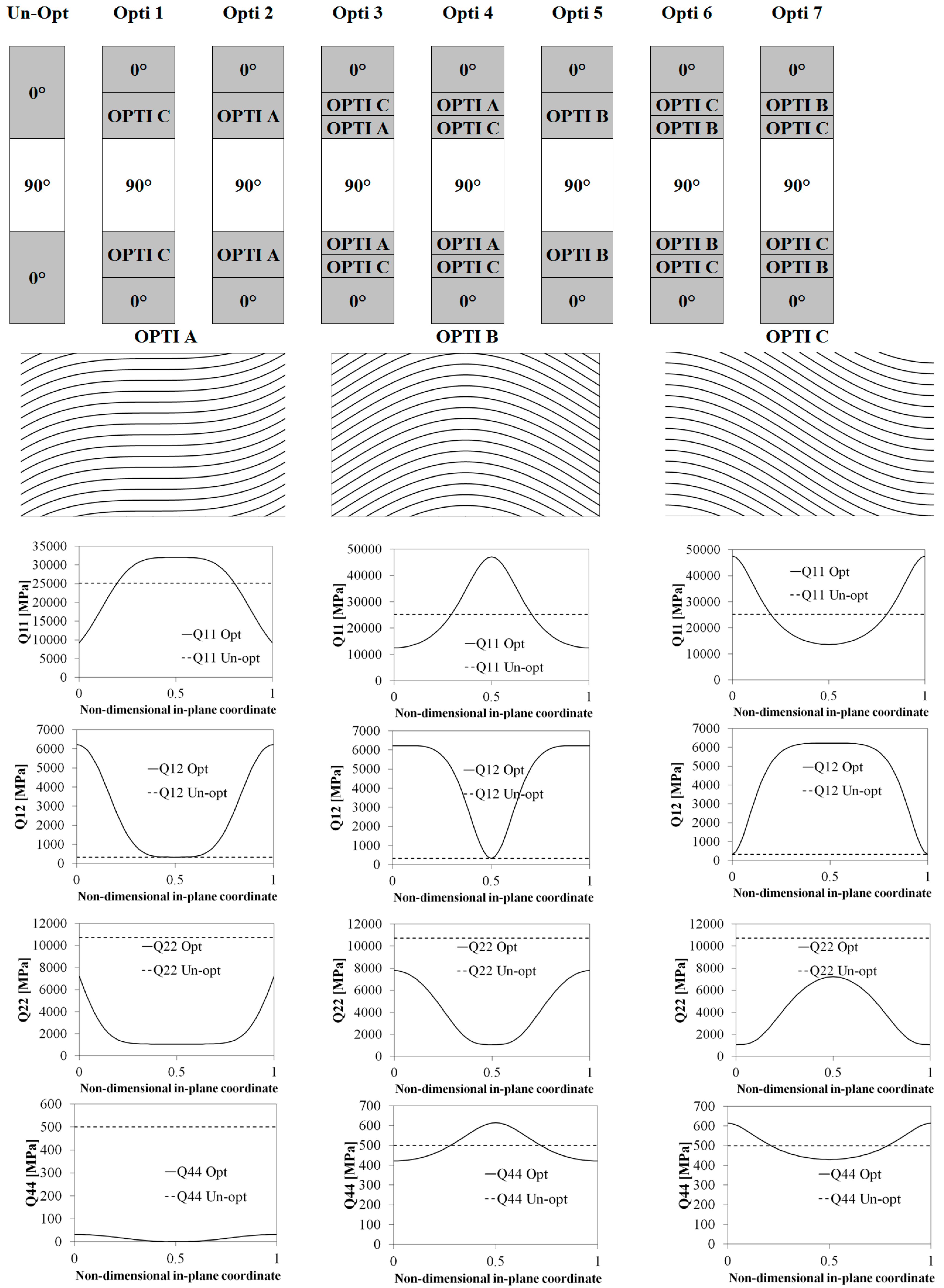
Figure 2.
Lay-ups considered for the optimization of the laminated plate and in-plane distributions of the optimized stiffness coefficients.
Figure 2.
Lay-ups considered for the optimization of the laminated plate and in-plane distributions of the optimized stiffness coefficients.
The unknown coefficients , , p, , , kx, ky in Equation (16) are computed by enforcing conditions such as the stiffness at the bounds of the domain and a convex or a concave shape, in order to determine whether the solution minimises or maximises the strain energy components. In addition, the solution has to be physically consistent, so it is necessary to enforce thermodynamic constraints related to the conservation of energy.
In order to make the algebraic manipulation easier and to meet the actual manufacturing technologies (e.g., automatic fibre placement [
14,
15]), the distributions of Equation (16) are approximated with sub-optimal polynomial expansions,
i.e.,
, where the order of expansion
G is determined considering accuracy as well as computational effort.
The unknown coefficients of the polynomial expansion are determined by imposing thermodynamic constraints and conditions such as the magnitude of the stiffness at the bounds of the domain, a convex or a concave shape and other conditions all coefficients reach saturation. Once the expressions of the optimal
Qij have been obtained, the optimal in-plane variation of the fibre orientation can be computed by inverting the stress-strain relations for lamina of arbitrary orientation (see [
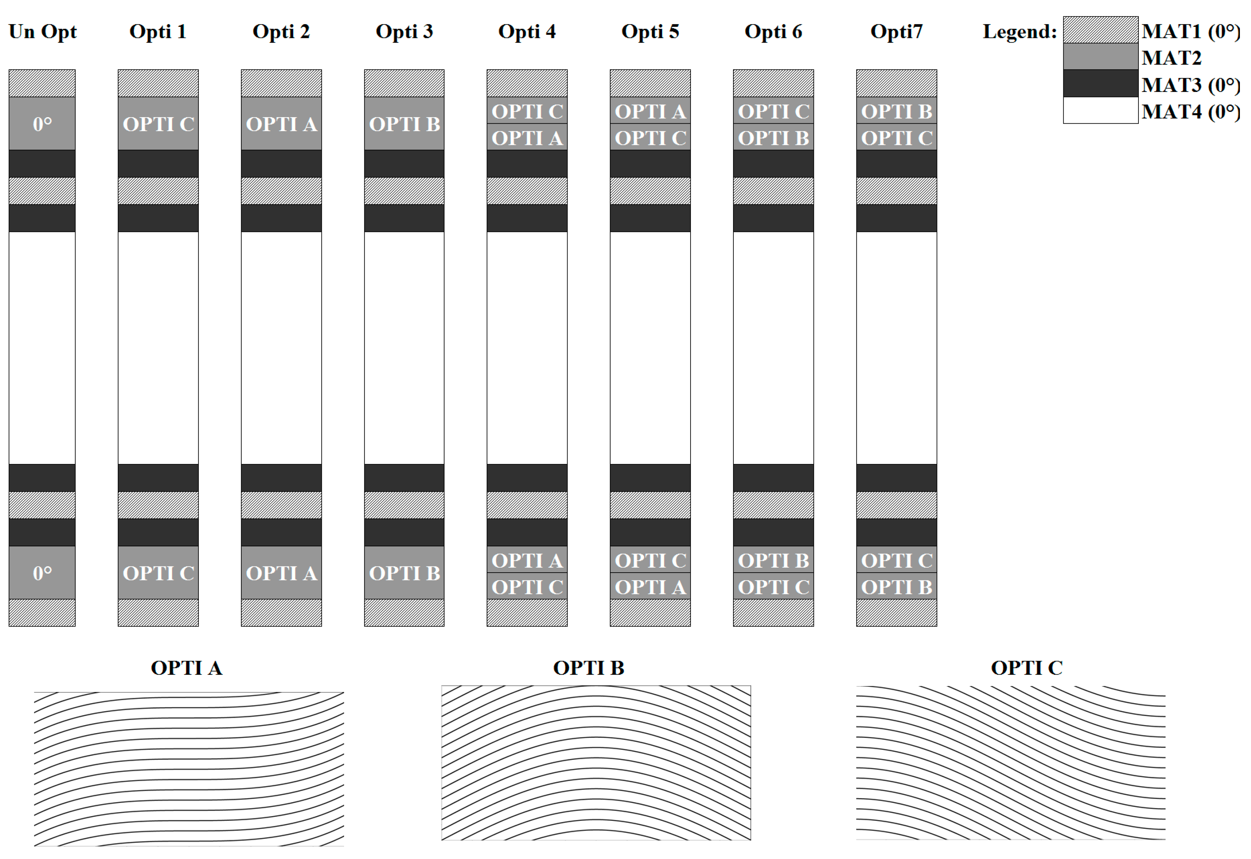
29]). In details, in the numerical applications, three sub-optimal distributions are considered: two that minimize the bending component of the strain energy (OPTI A and OPTI B), and one that minimizes the shear component of the strain energy (OPTI C) of each ply. From a practical viewpoint, OPTI A distribution is obtained by imposing maximum bending stiffness at the centre of the ply and minimum at the edge. The in-plane variations of the most significant
Qij for the OPTI A ply are reported in
Figure 2. From this figure, it can be seen that OPTI A determines a significant increase of
Q11 at the centre of the ply, and a reduction at its edges.
For what concerns Q12, which represents the local in-plane shear stiffness, its magnitude is significantly high at bounds of the ply, while at the centre it remains almost unchanged with respect to the straight fibre case. This trend is also the same of the coefficient Q22. The coupled effects of the distributions of Q11, Q12 and Q22 imply, as desired, an increase of the bending stiffness at the centre of the ply and a decrease at the bounds, where the shear stiffness in the in-plane direction grows. Instead, with OPTI A distribution, the transverse shear stiffness decreases, maintaining a value that is almost constant.
OPTI B, which has never been considered before in the previous applications of OPTI, is also obtained when imposing maximum bending stiffness at the centre of the ply and minimum at the edge, but in this case it is different from the sign of the concavity imposed at the edge of the ply. For what concerns the in-plane distributions of the stiffness coefficients reported in
Figure 2, the global behaviour is roughly the same described above for OPTI A. The only differences are due to a sharper variation with respect to the previous distributions and to a mean value of the transverse shear stiffness that is almost similar to that of the un-optimized layer. As a consequence, OPTI B determines a lower increase of the value of the bending stiffness with respect to OPTI A.
Finally, the OPTI C distribution is obtained imposing maximum bending stiffness at the edge of the ply and minimum at the centre, as shown by the stiffness distributions reported in
Figure 2. This figure shows that the in-plane distribution
Q11 is higher at the bounds than at the centre of the ply, while for
Q12 and
Q22 the trend is the opposite. In fact, they have low value at bounds and high value at the centre.
Q44 remains almost constant and similar to the un-optimized value. From the practical point of view, OPTI C distribution determines a transfer of energy from bending in the
x-direction to bending in the
y-direction and to in-plane shear.
It could be remarked that these distributions are similar to those obtained by other researchers (see, e.g., [
6,
30]). For the first time, in the numerical applications these optimized distributions (OPTI A, B and C) will be coupled in order to improve structural performances aiming to locally reduce stress concentrations, which are a serious design concern for laminates and sandwiches. The previous considerations form the physical background for the discussion of numerical results.
Note that after computation of the optimal in-plane variation of the fibre orientation, the optimal stacking sequence (i.e., OPTI 1–7) could be easily determined by hand (as done in the present paper) or by the classical optimization technique (gradient based search techniques or genetic algorithms).
It is noteworthy that sandwiches are treated as laminates, with the core assumed to be a thick intermediate layer, whose properties are computed from the cellular properties, as prescribed in [
31]. As a consequence, the complex interaction of faces and core and the intricate variation of the transverse displacements across the thickness of the highly deformable layers constituting the cores should be described by the zig-zag model. With this choice, it is possible to efficiently carry out optimization with the lowest computational effort, but accurately describing the structural response.
4. Numerical Applications
Once the accuracy of the model is also assessed for dynamic analyses, it is possible to focus the attention on the results obtained using optimized configurations. In particular, aiming at showing the effectiveness of the optimization procedure, applications to different kind of structures (beam, plate, laminate and sandwich) will be presented.
4.1. Optimization of a Laminated Plate
A laminated plate with a thickness ratio
S =
L/
h of 4 is considered because it is a severe test for the model, though it is an unrealistic case. The un-optimized material has the following properties:
EL/
ET = 25;
GLT/
ET = 0.5;
GTT/
ET = 0.2; υ
LT = 0.25; the thickness of the layers is [h/3,h/3,h/3], while the lay-ups considered are reported in
Figure 3. Please notice that the stacking sequence of the optimized lay-up is determined by directly comparing the response of all the stack-up possible options since few constituent layers are considered.
Table 2 reports the first five natural frequencies of the analyzed configurations.
Table 2.
Natural frequencies for a simply supported laminate incorporating variable optimized stiffness plies with length-to-thickness ratio 4.
Table 2.
Natural frequencies for a simply supported laminate incorporating variable optimized stiffness plies with length-to-thickness ratio 4.
| ω | Un-Opt | Opti 1 | Opti 2 | Opti 3 | Opti 4 | Opti 5 | Opti 6 | Opti 7 |
|---|
| ω1 | 7.04 | 7.68 | 7.16 | 7.55 | 7.35 | 7.16 | 7.18 | 7.21 |
| ω2 | 33.64 | 40.18 | 38.68 | 43.11 | 43.09 | 38.69 | 38.99 | 38.97 |
| ω3 | 38.57 | 50.41 | 39.86 | 46.52 | 43.94 | 39.72 | 39.80 | 39.07 |
| ω4 | 52.61 | 54.39 | 54.23 | 51.88 | 51.90 | 54.30 | 52.28 | 52.26 |
| ω5 | 65.84 | 59.09 | 66.22 | 61.66 | 63.01 | 65.88 | 63.39 | 63.90 |
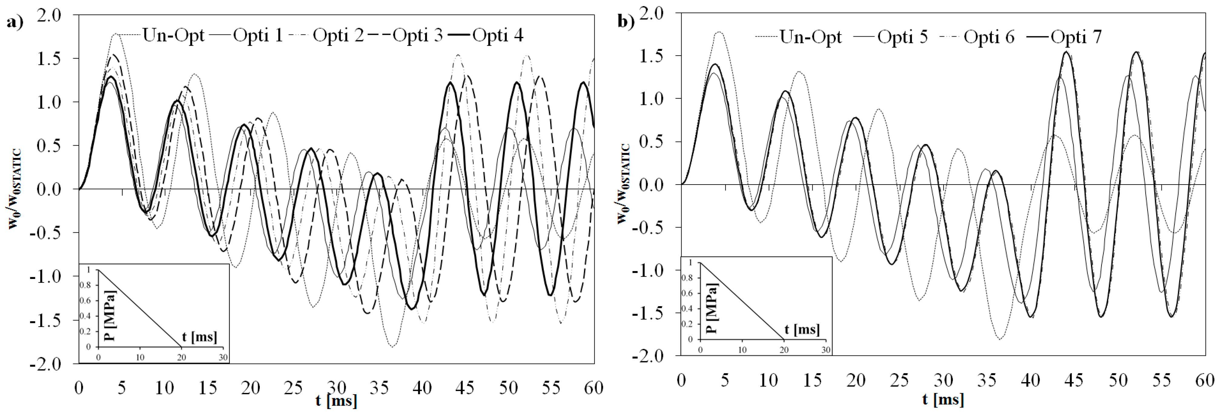
Figure 5 represents the central deflection of the optimized laminated plate normalized to the static one under triangular pulse loading.
Figure 5.
Non-dimensional deflection time history for all the optimized configurations.
Figure 5.
Non-dimensional deflection time history for all the optimized configurations.
Table 3 reports the interlaminar stresses at
t = 32 ms taken as an example for OPTI 4 and OPTI 7 configurations, which according to [
18] are normalized as:
where
P is the maximum of the applied load.
Table 3.
Normalized interlaminar stresses for configurations OPTI 4 and OPTI 7 of the simply supported laminate.
Table 3.
Normalized interlaminar stresses for configurations OPTI 4 and OPTI 7 of the simply supported laminate.
| z/h | UN OPT | OPTI 4 | OPTI 7 |
|---|
| σ*xz | σ*yz | σ*xz | σ*yz | Gainxz | Gainyz | σ*xz | σ*yz | Gainxz | Gainyz |
|---|
| −0.50 | 0.00E+00 | 0.00E+00 | 0.00E+00 | 0.00E+00 | 0.0% | 0.0% | 0.00E+00 | 0.00E+00 | 0.0% | 0.0% |
| −0.42 | 2.08E−02 | 3.22E−03 | 1.96E−02 | 3.44E−03 | −5.9% | 6.9% | 1.86E−02 | 3.36E−03 | −10.7% | 4.5% |
| −0.33 | 3.34E−02 | 5.72E−03 | 2.72E−02 | 5.87E−03 | −18.5% | 2.5% | 2.55E−02 | 5.74E−03 | −23.7% | 0.2% |
| −0.25 | 3.84E−02 | 8.97E−03 | 3.99E−02 | 7,48E−03 | 4.0% | −16.7% | 3.81E−02 | 7.28E−03 | −0.8% | −18.9% |
| −0.17 | 3.26E−02 | 9.87E−03 | 3.20E−02 | 1.47E−02 | −2.0% | 48.8% | 3.02E−02 | 1.30E−02 | −7.5% | 31.3% |
| −0.10 | 3.25E−02 | 2.37E−02 | 3.18E−02 | 2.67E−02 | −2.1% | 12.4% | 3.00E−02 | 2.44E−02 | −7.7% | 2.6% |
| −0.03 | 3.23E−02 | 3.08E−02 | 3.16E−02 | 3.28E−02 | −2.2% | 6.6% | 2.98E−02 | 3.02E−02 | −7.8% | −2.0% |
| 0.03 | 3.21E−02 | 3.12E−02 | 3.15E−02 | 3.33E−02 | −2.1% | 6.8% | 2.96E−02 | 3.06E−02 | −7.8% | −1.8% |
| 0.10 | 3.19E−02 | 2.50E−02 | 3.13E−02 | 2.82E−02 | −2.0% | 13.0% | 2.95E−02 | 2.57E−02 | −7.7% | 3.1% |
| 0.17 | 3.17E−02 | 1.19E−02 | 3.11E−02 | 1.73E−02 | −1.8% | 44.8% | 2.93E−02 | 1.53E−02 | −7.5% | 28.1% |
| 0.25 | 3.76E−02 | 1.07E−02 | 2.60E−02 | 1.59E−02 | −30.8% | 48.9% | 3.78E−02 | 7.22E−03 | 0.6% | −32.3% |
| 0.33 | 3.28E−02 | 6.71E−03 | 1.27E−02 | 5.87E−03 | −61.4% | −12.5% | 2.94E−02 | 5.25E−03 | −10.4% | −21.8% |
| 0.42 | 2.04E−02 | 3.85E−03 | 3.90E−03 | 3.44E−03 | −80.9% | −10.5% | 2.32E−02 | 2.45E−03 | 13.4% | −36.3% |
| 0.50 | 0.00E+00 | 0.00E+00 | 0.00E+00 | 0.00E+00 | 0.0% | 0.0% | 0.00E+00 | 0.00E+00 | 0.0% | 0.0% |
As it can be seen, the use of optimized ply considerably reduces the interlaminar stresses, without significant stiffness loss. This result is consequent to the fact that plies of type OPTI A, B and C are incorporated, which, as described previously, produce a transfer of energy from shear and bending in the x-direction, to bending in the y-direction and to in-plane shear. The best lay-ups are OPTI 4 and OPTI 7, which are characterized by the simultaneous presence of plies that minimize the bending component of the strain energy and of plies that minimize the shear component of the strain energy. In particular, the highest reduction of the shear stress at the critical interfaces is obtained placing OPTI C plies near the interfaces. This is physically consistent, since with this stacking sequence the difference between the material properties of adjacent plies is reduced.
4.2. Optimization of a Sandwich Plate
Now a simply supported sandwich square plate is considered. The plate is characterized by a thickness ratio
S of 4 and the properties of the un-optimized materials are: MAT 1:
E1 =
E3 = 1 GPa,
G13 = 0.2 GPa, υ
13 = 0.25; MAT 2:
E1 = 33 GPa,
E3 = 1 GPa,
G13 = 0.8 GPa, υ
13 = 0.25; MAT 3:
E1 = 25 GPa,
E3 = 1 GPa,
G13 = 0.5 GPa, υ
13 = 0.25; MAT 4:
E1 =
E3 = 0.05 GPa,
G13 = 0.0217 GPa, υ
13 = 0.15. According to what previously discussed, the sandwich plate is simulated as a multilayered plate and the thickness of the layers is [0.010,0.025,0.015,0.020,0.030,0.4]
s, while the lay-ups considered are reported in
Figure 6.
Figure 6.
Lay-ups considered for the optimization of the sandwich plate.
Figure 6.
Lay-ups considered for the optimization of the sandwich plate.
It should be noted that in all the lay-ups considered, the optimized plies are those realized with MAT2. In fact, MAT2, which has the highest tensile modulus, determines a sharp variation of the mechanical properties across the thickness of the structure. Therefore the insertion of optimized layers is an attempt to reduce the difference with the adjacent layers, keeping the bending stiffness unchanged.
Table 4 reports the first five natural frequencies of the analyzed configurations.
Table 4.
Natural frequencies for a simply supported sandwich incorporating variable optimized stiffness plies with length-to-thickness ratio 4.
Table 4.
Natural frequencies for a simply supported sandwich incorporating variable optimized stiffness plies with length-to-thickness ratio 4.
| ω | Un-Opt | Opti 1 | Opti 2 | Opti 3 | Opti 4 | Opti 5 | Opti 6 | Opti 7 |
|---|
| ω1 | 5.39 | 6.53 | 6.11 | 5.85 | 6.34 | 6.32 | 6.10 | 6.13 |
| ω2 | 16.93 | 24.82 | 21.58 | 23.10 | 23.62 | 23.61 | 23.22 | 23.23 |
| ω3 | 20.17 | 32.10 | 28.36 | 25.84 | 30.88 | 30.87 | 27.26 | 27.21 |
| ω4 | 58.03 | 52.93 | 59.25 | 58.23 | 56.05 | 56.05 | 55.77 | 55.77 |
| ω5 | 59.82 | 57.24 | 61.67 | 60.03 | 59.11 | 59.11 | 57.83 | 57.83 |
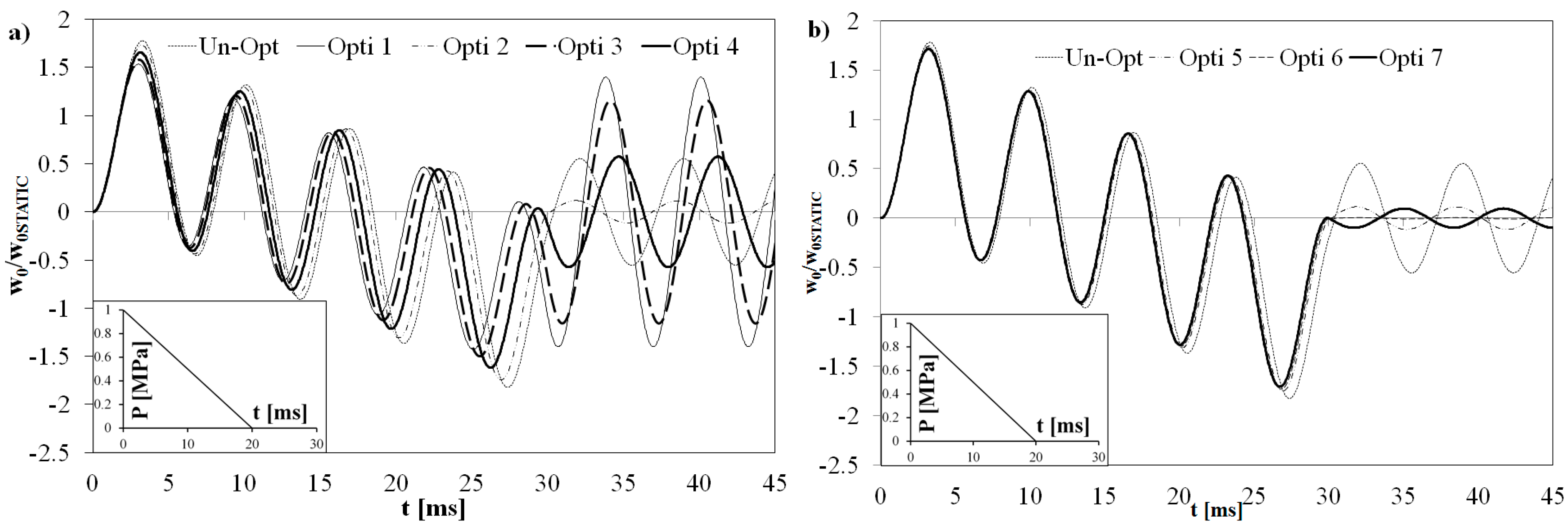
Figure 7 represents the central deflection of the optimized plate normalized to the static one under triangular pulse loading.
Figure 7.
Non-dimensional deflection time history for all the optimized configurations.
Figure 7.
Non-dimensional deflection time history for all the optimized configurations.
Table 5 reports the interlaminar stresses at
t = 43 ms for OPTI 3 and OPTI 7 configurations, according to [
18], normalized as:
From the reported results it can be seen that, in contrast to what happens for the laminated plate, the presence of optimized layers in the sandwich plate reduces the amplitude of the central deflection at the beginning of the time history. On the contrary, as time unfolds, the amplitude of the central deflection for the un-optimized plate is smaller than those of the optimized configurations. However, remembering that the aim of the optimization process is the reduction of the interlaminar stresses, it can be observed that this target is also completely achieved for sandwiches subjected to blast pulse loading, as shown in
Table 5.
Table 5.
Normalized interlaminar stresses for configurations OPTI 3 and OPTI 7 of the simply supported sandwich.
Table 5.
Normalized interlaminar stresses for configurations OPTI 3 and OPTI 7 of the simply supported sandwich.
| z | UN OPT | OPTI 3 | OPTI 7 |
|---|
| σ*xz | σ*yz | σ*xz | σ*yz | Gainxz | Gainyz | σ*xz | σ*yz | Gainxz | Gainyz |
|---|
| −0.50 | 0.00E+00 | 0.00E+00 | 0.00E+00 | 0.00E+00 | 0.0% | 0.0% | 0.00E+00 | 0.00E+00 | 0.0% | 0.0% |
| −0.42 | 1.50E−02 | 2.51E−02 | 8.51E−03 | 1.09E−02 | −43.1% | −56.6% | 8.20E−03 | 1.12E−02 | −45.2% | −55.5% |
| −0.33 | 3.64E−01 | 1.08E−01 | 3.61E−01 | 4.37E−02 | −0.7% | −59.4% | 3.02E−01 | 1.07E−01 | −17.0% | −0.4% |
| −0.25 | 4.49E−01 | 1.42E−01 | 4.10E−01 | 5.43E−02 | −8.5% | −61.8% | 3.49E−01 | 2.11E−01 | −22.2% | 48.7% |
| −0.17 | 4.61E−01 | 1.75E−01 | 4.13E−01 | 6.14E−02 | −10.5% | −64.9% | 3.52E−01 | 2.20E−01 | −23.7% | 26.0% |
| −0.10 | 3.34E−01 | 2.18E−01 | 2.58E−01 | 6.13E−02 | −22.9% | −71.9% | 2.17E−01 | 2.25E−01 | −35.0% | 3.0% |
| −0.03 | 3.30E−01 | 2.24E−01 | 2.48E−01 | 5.39E−02 | −24.8% | −76.0% | 2.08E−01 | 2.18E−01 | −36.9% | −2.8% |
| 0.03 | 3.25E−01 | 2.20E−01 | 2.43E−01 | 4.92E−02 | −25.2% | −77.6% | 2.02E−01 | 2.12E−01 | −37.7% | −3.7% |
| 0.10 | 3.11E−01 | 1.96E−01 | 2.34E−01 | 3.77E−02 | −24.8% | −80.7% | 1.89E−01 | 1.93E−01 | −39.1% | −1.6% |
| 0.17 | 4.39E−01 | 1.52E−01 | 3.88E−01 | 3.63E−02 | −11.6% | −76.1% | 2.96E−01 | 1.73E−01 | −32.5% | 13.5% |
| 0.25 | 4.25E−01 | 1.19E−01 | 3.83E−01 | 2.76E−02 | −9.7% | −76.7% | 2.88E−01 | 1.54E−01 | −32.2% | 30.1% |
| 0.33 | 3.40E−01 | 8.41E−02 | 3.34E−01 | 3.38E−02 | −2.0% | −59.8% | 2.27E−01 | 1.35E−01 | −33.3% | 60.2% |
| 0.42 | 1.51E−02 | 1.92E−03 | 1.06E−02 | 1.88E−03 | −29.7% | −2.3% | 1.43E−02 | 1.84E−03 | −4.9% | −4.6% |
| 0.50 | 0.00E+00 | 0.00E+00 | 0.00E+00 | 0.00E+00 | 0.0% | 0.0% | 0.00E+00 | 0.00E+00 | 0.0% | 0.0% |
4.3. Local Optimization
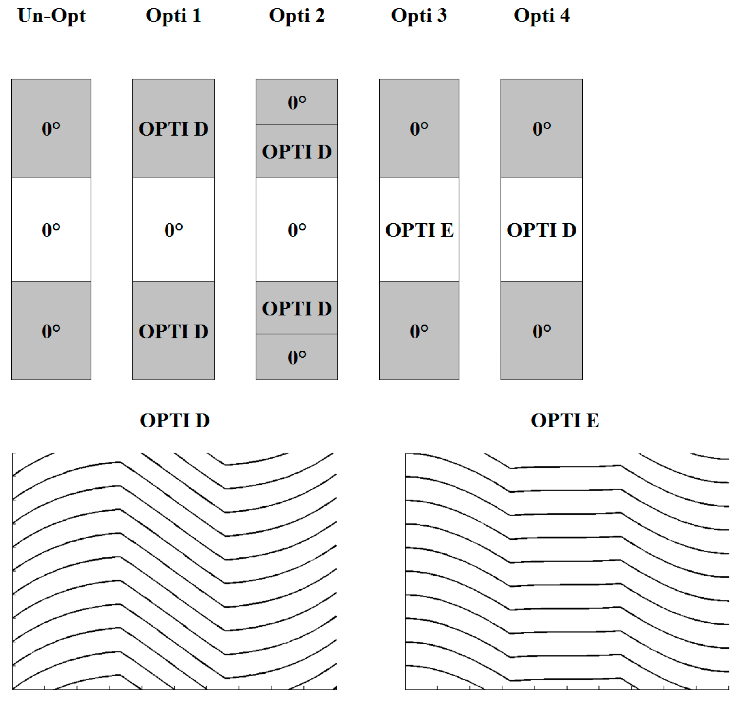
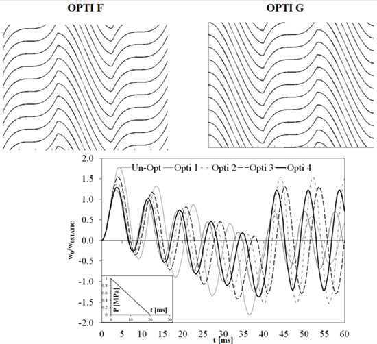
Having shown the great advantages achieved with the insertion of optimized plies, local optimization is now considered, with the aim of minimizing local effects. In order to study this, the optimized distributions of OPTI A, OPTI B and OPTI C are coupled. Accordingly, the ply is divided in three zones in the in-plane direction, and in each zone the fibre distribution varies. In particular the four distributions reported in
Figure 1 have been considered. They are obtained respectively by (starting from the left):
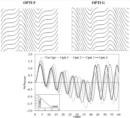
For OPTI D and OPTI E the period of the fibre distributions is the length of the ply, while for OPTI F and OPTI G the period is 1/3 of the length of the ply. According to the stiffness distributions discussed in
Section 3, concerning OPTI D,
Q11 and
Q12 are quite large across the two parts corresponding to OPTI A, while they drop in the central zone of the ply. The transverse shear stiffness
Q44 is slightly constant in the outer portion of the ply, while it decreases at the centre. As a result, once an OPTI D ply is incorporated into the lay-up, it decreases the bending stiffness at the centre, where it increases the in-plane and transverse shear stiffness. It behaves exactly in the opposite way in the outer portions of the layer. Instead, OPTI E increases the stiffness coefficients that OPTI D decreases, and it does the contrary where OPTI D leads to an increase.
OPTI F and OPTI G determine the same in-plane variations in stiffness reported in
Figure 3 but at a length that is 1/3 of the ply, which therefore has the opposite behaviour in different zones.
4.3.1. Local Optimization of a Laminated Beam
First of all, a simply supported laminated beam subjected to a sinusoidal loading is analysed. The beam is characterized by a thickness ratio
S of 10 and the properties of the un-optimized material are:
EL/
ET = 25;
GLT/
ET = 0.5;
GTT/
ET = 0.2; υ
LT = 0.25. The thickness of the layers is [h/3,h/3,h/3], while the lay-ups considered are reported in
Figure 8.
Figure 8.
Lay-ups considered for the local optimization of the laminated beam.
Figure 8.
Lay-ups considered for the local optimization of the laminated beam.
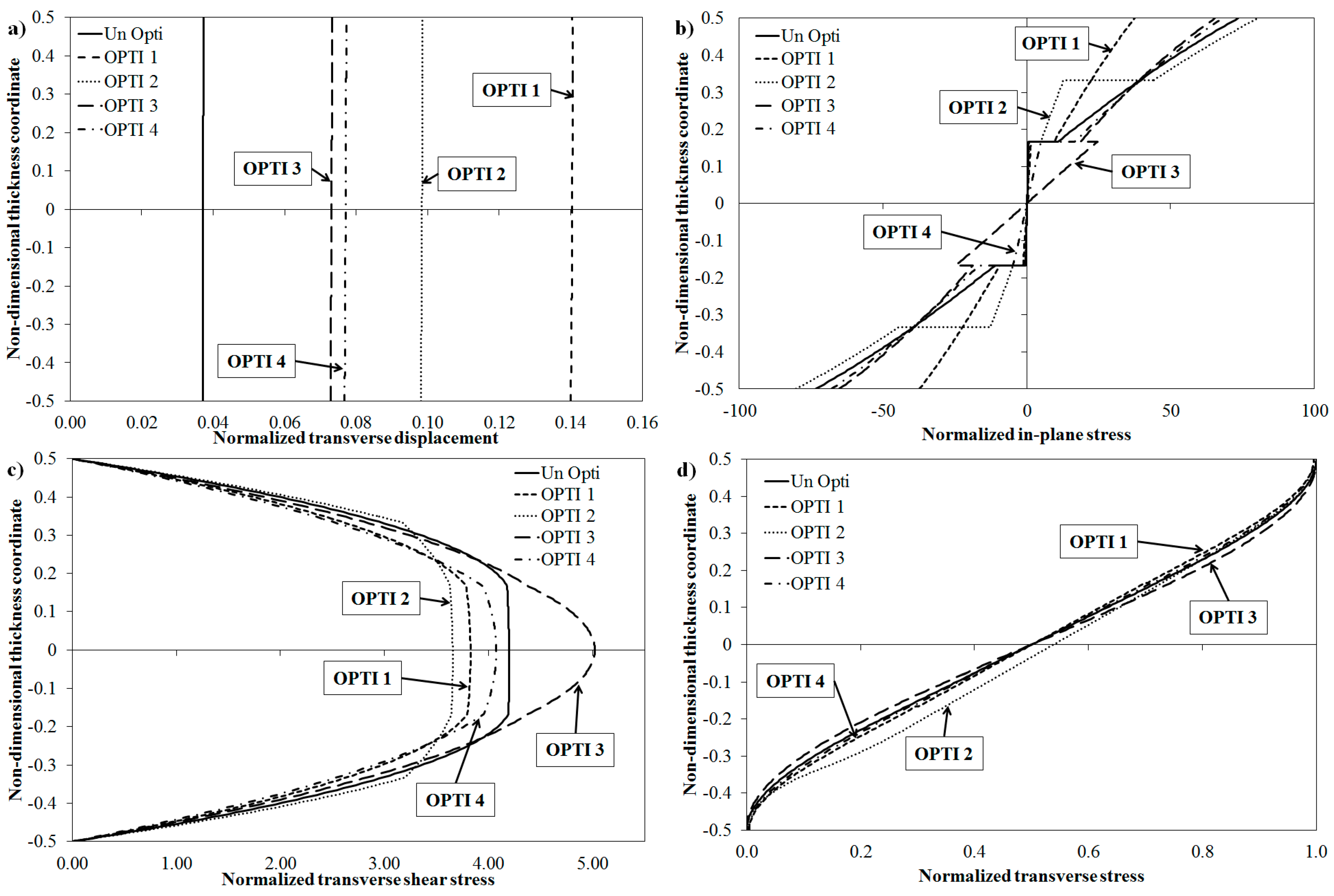
The transverse displacement, the in-plane, the shear and the transverse normal stresses are reported in
Figure 9, normalized as follows:
It can be noted that, except for the OPTI 3 lay-up, the optimization process reduces the interlaminar stress, while the transverse normal stress does not considerably vary in all the analysed cases. The insertion of optimized plies reduces the bending stiffness of the laminate; in fact the transverse displacement for all the optimized lay-ups is higher than that of the un-optimized one. As discussed above, the optimization procedure determines a transfer of energy from one mode to another; as a result, a small increase of the in-plane stress can be obtained as shown in
Figure 9b. This does not represent a design concern since the in-plane strength of composites is much greater than the out-of-plane strength.
Figure 9.
Through the thickness variation of (a) transverse displacement, (b) in-plane stress, (c) transverse shear stress, and (d) transverse normal stress for the optimization of a laminated plate.
Figure 9.
Through the thickness variation of (a) transverse displacement, (b) in-plane stress, (c) transverse shear stress, and (d) transverse normal stress for the optimization of a laminated plate.
4.3.2. Local Optimization of a Sandwich Beam
Also, a simply supported sandwich beam under sinusoidal loading is considered. The beam is characterized by a thickness ratio
S of 10 and the properties of the un-optimized materials are: MAT FACE:
E1 = 25 GPa,
E3 = 1 GPa,
G13 = 0.5 GPa, υ
13 = 0.25; MAT CORE:
E1 =
E3 = 0.05 GPa,
G13 = 0.0217 GPa, υ
13 = 0.15. The thickness of the layers is [0.2,0.3]
s, while the lay-ups considered are reported in
Figure 1.
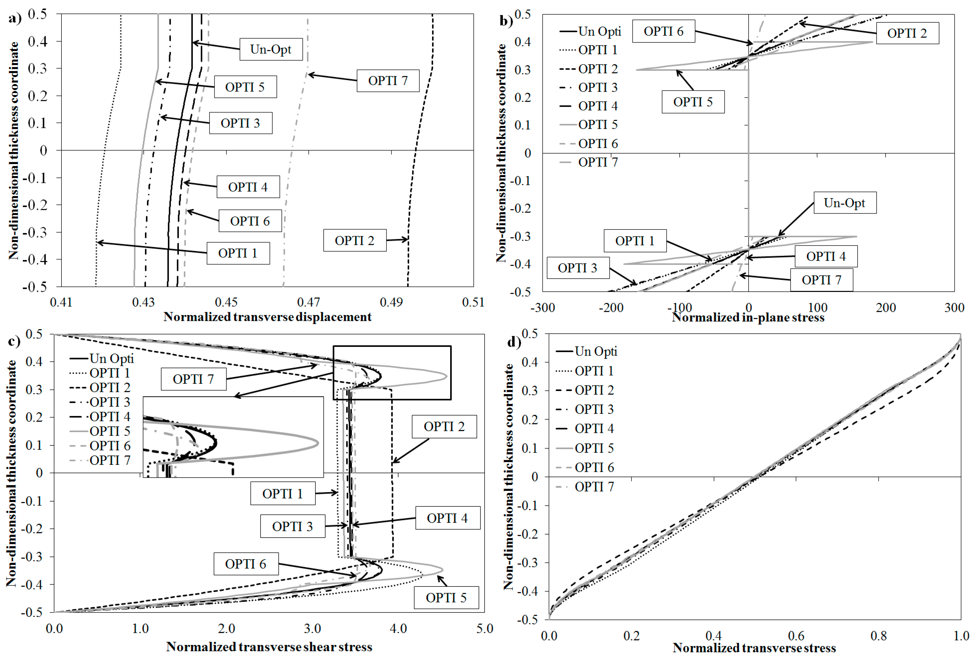
The transverse displacement, the in-plane, the shear and the transverse normal stresses are reported in
Figure 10, where they are normalized according to Equation (26).
As for the laminated beam, the transverse normal stress does not considerably vary with the insertion of optimized layers, while considering the shear stress the behaviour is different between the lay-ups considered. For the OPTI 1 configuration a decrease can be seen (−4.1%) in the shear stress at the interface, while its maximum value grows (+20%). OPTI 2 does not determine an improvement with respect to the un-optimized configuration. OPTI 3 and OPTI 4 produce a small decrease (about 1%) of the maximum value of the shear stress, as well as its value at the interface. OPTI 5 produces a great increase in the maximum value of the magnitude of the shear and of the in-plane stress. However, these are not significant problems, since the in-plane strength and the shear strength in the faces are high. OPTI 6 is the best configuration for reducing the maximum value of the shear stress (−7.63%) and of the in-plane stress at the interface (about −80%). Its effect on the shear stress at the interface is limited (+0.96%). OPTI 7 reduces the maximum value of the shear and of the in-plane stress (−15.17% and −61.3% respectively).
Figure 10.
Through the thickness variation of (a) transverse displacement, (b) in-plane stress, (c) transverse shear stress, and (d) transverse normal stress.
Figure 10.
Through the thickness variation of (a) transverse displacement, (b) in-plane stress, (c) transverse shear stress, and (d) transverse normal stress.
5. Concluding Remarks
An optimization technique has been applied to laminates and sandwiches undergoing static and blast pulse pressure loading. The aims are to reduce the detrimental effects at the critical interfaces and those due to impulsive loading, which can lead to premature failure of the structures.
The technique provides the spatial distribution of the stiffness properties in closed form as the solution for Euler–Lagrange equations obtained minimizing the transverse shear energy and maximizing the bending energy under spatial variation of the stiffness properties The optimization procedure and the computation of the response of sandwich panels have been performed in analytical form using a refined zig-zag model with hierarchic representation of displacements across the thickness. This model accurately captures the transverse shear deformations and the out-of-plane stresses directly from constitutive equations with a much lower computational effort than the currently available high-order layerwise models.
As a result of the tailoring optimization, three curvilinear paths of fibre have been obtained: OPTI A and OPTI B, which minimize the bending component of the strain energy, and OPTI C, which minimizes the shear component of the strain energy in a generic ply. These fibre distributions determine a transfer of energy from shear and bending in the x-direction to bending in the y-direction and to in-plane shear, which are not serious design concerns, as composites have high in-plane strengths.
Numerical applications have shown that, using these optimized plies, it is possible to recover stresses at the critical interfaces. Of course, the most evident stress reductions at the interfaces have been obtained by placing OPTI C plies near them, thus mitigating the variation of mechanical properties between adjacent layers. Finally, new applications regarding local optimization have been presented, aimed at a reduction of local effects, which is one of the most serious design concerns. In particular, laminated and sandwich beams subjected to sinusoidal loading have been considered. The numerical results show a reduction of the interlaminar shear stress in both cases.


