
A Weighted Feature Fusion Model for Unsteady Aerodynamic Modeling at High Angles of Attack

1
School of Aerospace Engineering, Xiamen University, Xiamen 361102, China
2
Aerospace System Engineering Shanghai, Shanghai 201109, China
*
Author to whom correspondence should be addressed.
Aerospace 2024, 11(5), 339; https://doi.org/10.3390/aerospace11050339
Submission received: 21 March 2024
/
Revised: 18 April 2024
/
Accepted: 22 April 2024
/
Published: 25 April 2024
Abstract
:Unsteady aerodynamic prediction at high angles of attack is of great importance to the design and development of advanced fighters. In this paper, a weighted feature fusion model (WFFM) that combines the state-space model and neural networks is proposed to build an unsteady aerodynamic model for the precise simulation and control of post-stall maneuvers. In the proposed model, the influences of the physical model on neural networks are considered and adjusted by introducing a standardization layer and a new weighting method. A long short-term memory (LSTM) network is used to fuse two mappings: one from flight states to aerodynamic loads, and the other from low-fidelity data to high-fidelity data. Data from wind tunnel oscillation experiments at high angles of attack using a new kind of wire-driven parallel robot and the traditional tail support are used for verifying the proposed aerodynamic model. The output of the WFFM is also compared with predictions from other models, such as the state-space model, single LSTM model, and feature fusion model not including a feature weighting layer. Results demonstrate improved accuracy of the proposed model in the interpolation and extrapolation tests. Furthermore, the WFFM is applied to the flight simulation of F-16 with different control inputs. Compared with conventional models, the WFFM shows improved accuracy and better generalization capability.
1. Introduction
Despite the increasing prevalence of advanced beyond-visual-range missiles, close-range dogfights remain a critical aspect of aerial combat. High agility and maneuverability are still the indispensable key features of next-generation fighter aircraft. The aerodynamic characteristics of aircraft at high angles of attack exhibit highly nonlinear and unsteady characteristics due to phenomena such as flow separation and vortex shedding. The traditional database-based interpolation method is no longer sufficient for the precise simulation and control of post-stall maneuvers. Therefore, the establishment of accurate aerodynamic models is crucial for aircraft dynamics investigation, stability analysis, and control system design at high angles of attack. Past work has focused on mathematical models. These models establish a mathematical relationship between aerodynamic loads and flight states (such as velocity, angle of attack, and sideslip angle) based on unsteady flow phenomena and physical principles, such as the dynamic derivative model [1,2], the state-space model [3,4], and the indicial function model [5,6]. While these models often possess explicit physical interpretations, their accuracy is constrained by the level of understanding of physical phenomena and the degree of mathematical simplification involved.
In recent years, with the rapid advancement of artificial intelligence, machine learning models have found widespread application in unsteady aerodynamic modeling. Machine learning models, also known as black-box models, bypass the need for explicating complex physical mechanisms. With a sufficient amount of training data, these models possess powerful nonlinear fitting capabilities to establish the relationship between flight states and aerodynamic loads. Models such as support vector machines [7,8], random forest [9], and neural networks [10,11,12] have been employed for this purpose. Furthermore, recurrent neural networks improve accuracy by capturing the time lag effects of unsteady aerodynamics [13,14,15]. In addition to flight state data, the geometric representation of the airfoils is used as an input feature for the deep neural network to obtain the aerodynamic parameters [16,17]. While machine learning models can fit nonlinear relationships effectively, they cannot provide a reasonable explanation for how inputs are used to make predictions.
If the explanation of physical relationships between flight states and aerodynamic loads could be applied to model training, it would enable the model to possess the interpretability of traditional mathematical models and the powerful nonlinear fitting capabilities of black-box models simultaneously. Currently, there are two approaches to exploring the combination of traditional mathematical models and black-box models.
One approach involves using physics-informed neural networks (PINNs) [18]. The physics equations are incorporated into the loss function of a neural network to constrain the model while training, thereby ensuring outputs follow known physical laws [19]. Zhao et al. [20] proposed an identification method of aerodynamic models using a physics neural network that incorporates the attitude dynamics of an aircraft. Li et al. [21] utilized a PINN model to predict parameters of the state-space model using neural networks instead of predicting aerodynamics directly. While this method enhances the neural network’s extrapolation capabilities, it remains fundamentally a state-space model, with no significant improvement in interpolation accuracy.
Another approach is using the fusion model, which attempts to integrate traditional mathematical models into machine learning models [22]. The combination of models with different accuracy is also known as the multi-fidelity method. Low-fidelity models’ predictions, which are assumed to have similar trends to the high-fidelity models’ predictions, are used to provide additional information. Wang [23] and Li, et al. [24] combined dynamic derivative models with black-box models for unsteady aerodynamic prediction. These are used to compute low- and high-fidelity outputs, respectively. Finally, the least squares method is used to merge the outputs. The fusion model exhibited superior generality when compared to black-box models. However, the effectiveness of the least squares method depends on the correlation between models and the assumptions about the error distribution. If the models are highly correlated, the least squares method may not provide a significant advantage. Zhang et al. [25] presents an innovative aerodynamic modeling method using heterogeneous data and physical feature embedding, significantly improving prediction accuracy while reducing training data needs. The complexity of implementation, reliance on high-quality data, need for further real-world validation, and demand for substantial computational resources may be potential challenges of this approach.
This paper proposes a weighted feature fusion model (WFFM) based on the state-space model and long short-term memory network (LSTM) to predict nonlinear unsteady aerodynamics. The main contributions of this paper can be summarized as follows:
- (1)
- An architecture of an aerodynamic model is proposed, which combines the physics model and black-box model, exhibiting high accuracy in both interpolation and extrapolation tests.
- (2)
- A new method for weighting data is proposed. To reduce the impact of the state-space model error, the feature standardization layer and weighting layer, which is implemented using a single neuron and an activation function, are introduced.
- (3)
- Two mappings are established and fused by LSTM. One is the mapping from flight states to aerodynamic loads, and the other is the mapping from low-fidelity data to high-fidelity data.
- (4)
- To test the model, the proposed model is used to predict aerodynamic loads at high-angles-of-attack oscillations. Furthermore, the model is applied to a flight simulation of the F-16 with different control inputs to evaluate the generalization capability.
The paper is organized as follows. In Section 2, a brief introduction to the state-space method and neural network approach in aerodynamic modeling is given, and the structure of the WFFM based on the state-space model and LSTM is discussed in detail. In Section 3.1, the WFFM is used to predict the pitching moment coefficient at a high-angle-of-attack oscillation data obtained from wind tunnel experiments using a wire-driven parallel robot with eight wires (WDPR-8) and a traditional tail support to verify the proposed aerodynamic model. The results are then compared with three other models. In Section 3.2, the WFFM is applied to flight simulation and tested with different control inputs to validate the robustness and generalization of the models. Finally, Section 4 presents conclusions.
2. Modeling Methods
2.1. State-Space Method
Aircraft exhibit unsteady characteristics at high angles of attack, with airflow separation being a primary cause of aerodynamic time delays. To address this issue, Goma et al. proposed a state-space modeling method by introducing internal state-space variables into traditional aerodynamic derivative models [26]. The internal state-space variable is defined as the nondimensional coordinates of the airflow separation point, formulated as . Here, represents the distance between the position of the separation point and the leading edge of the airfoil, and represents the chord length. The range of values of the airflow separation point is . Introducing the airflow separation point allows the state-space model to depend not only on the instantaneous state variables but also on the physical mechanisms of airflow separation and attachment. The aerodynamic force and moment coefficients can be expressed as:
where represents the aerodynamics coefficients, represents the static component of aerodynamic coefficients, represents the dynamic component of aerodynamic coefficients, and represents the effect of control surface deflection on aerodynamic coefficients. In the state-space models, these coefficients are expanded in their Taylor series, using the first derivatives only and truncating higher-order terms, which may lead to insufficient accuracy. For example, considering the aerodynamic coefficient along the body axis, its dynamic aerodynamic coefficient is typically approximated by the first five terms of its Taylor series expansion:
In this formula, all coefficients of the expansion terms in the dynamic aerodynamic coefficients are approximated using a quadratic polynomial model. For example, can be expressed as follows:
where , , and are unknown parameters within the model, which are determined using parameter identification techniques.
2.2. Neural Network Approach
Neural networks are powerful machine learning tools capable of learning complex nonlinear relationships from data. They have found widespread applications in fields such as image recognition, natural language processing, and time-series prediction. A neural network consists of multiple layers of neurons, including an input layer, one or more hidden layers, and an output layer. All the neurons connected by links take in some data and use it to perform specific operations and generate output through an activation function.
Aerodynamic loads could be regarded as a function of the instantaneous values of the aircraft’s motion state variables [27]. In general, aerodynamic force and moment coefficients can be expressed as:
where is a vector of flight states.
Assuming the considered flight states include angle of attack , sideslip angle , pitch rate , altitude , and Mach number , then . A typical neural network used to predict aerodynamic loads is shown in Figure 1. By training a neural network on an aerodynamic dataset, it is possible to fit the mapping between flight states and aerodynamic loads, thereby achieving aerodynamic force and moment coefficients prediction.
The nonlinear and unsteady aerodynamics exhibit time lag effects. The unsteady aerodynamic forces and moments not only depend on the instantaneous states but also their time histories. Consequently, aerodynamic coefficients can be further modeled as a function of flight states over a continuous period:
where denote the flight states corresponding to the time step from to .
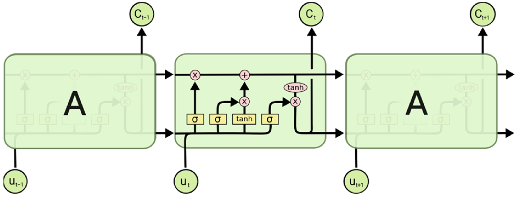
A recurrent neural network (RNN) is a type of neural network which uses sequential data or time series data. In contrast to the feedforward neural network, an RNN has feedback connections that enable the network to remember the previous input. Improved network structures such as Long Short-Term Memory (LSTM) and Gated Recurrent Units (GRUs) have resolved the vanishing gradient problem of traditional RNNs. Therefore, by inputting a continuous sequence of flight states into an RNN, it is possible to extract temporal information and improve the accuracy of machine learning models in aerodynamic forces and moments prediction. Figure 2 illustrates the process of using LSTM to predict aerodynamic loads based on the flight state history.
In summary, neural network models typically achieve high accuracy. However, the prediction process of neural networks is difficult to interpret, making their application in aerodynamic modeling challenging.
2.3. Weighted Feature Fusion Model
This paper introduces a weighted feature fusion model (WFFM) based on both the state-space model and LSTM. The design of the WFFM aims to overcome the difficulty of obtaining explicit physical mechanisms and high accuracy.
State-space models possess explicit physical meanings and describe the physical characteristics of separated flows. However, their limited fitting capability on nonlinear problems leads to low prediction accuracy. The aerodynamic data obtained through this method are often referred to as low-fidelity data. In contrast, the aerodynamic data obtained through methods such as wind tunnel experiments are referred to as high-fidelity data. The key concept behind the WFFM is to introduce physical information from the low-fidelity model into the neural network model. By using high-fidelity data for training, it establishes a mapping from low-fidelity data to high-fidelity data. This method minimizes the impact of errors in the low-fidelity data on prediction accuracy. In this way, the WFFM maintains physical significance and reduces additional errors to improve the accuracy of predictions for aerodynamic forces and moments.
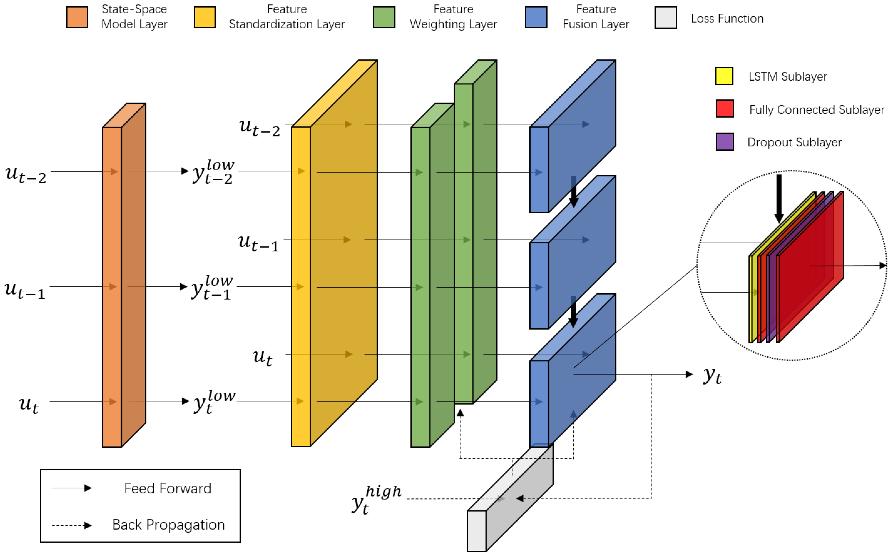
The structure of the WFFM is illustrated in Figure 3. The WFFM consists of four layers. The first layer is the state-space model layer, which takes flight states at time as input and calculates the low-fidelity aerodynamic coefficients using the state-space model:
where is the state-space model described in Section 2.1.
The second layer is the feature standardization layer, which makes the distributions of each feature in the input data have zero means and unit variances. This step normalizes the range of independent variables or features of data, thus improving training convergence speed and prediction accuracy [28]. The standardization operation is defined as follows:
where and represent the population of flight state data and low-fidelity data. and are the means of and , respectively. and are the standard deviations of and , respectively. and are the standardized data.
The third layer is the feature weighting layer. The process of weighting is used to assign different levels of importance to the various features in a dataset. Since the low-fidelity model output exhibits similar trends to the high-fidelity data, but with different values, it should be assigned a reduced weight to play a guiding role. The feature weighting layer is implemented using a single neuron and an activation function:
where and are the weight vector and bias term for this neuron, adjusted automatically through backpropagation based on the error between the predicted output and the actual high-fidelity output [29]. The activation function transforms any input from the range to a value that lies on the interval . and represent the weighted data.
The fourth layer is the feature fusion layer, which consists of the LSTM model. In this layer, two mappings have been established. One is the mapping from flight states to aerodynamic loads, which is the same as the black-box model. The other is the mapping from low-fidelity data to high-fidelity data, which includes additional physical information. The LSTM model with strong nonlinear fitting capabilities is used to fuse the features:
where represents the LSTM model, consisting of an LSTM sublayer with 100 hidden units, followed by two fully connected sublayers with 100 and 50 neurons, respectively, and a dropout layer. and compose the input vector for the LSTM model at time (). represents the output of the WFFM.
Finally, the error between the model’s output and the high-fidelity data is calculated. Based on the chain rule, the backpropagation algorithm calculates the error gradient of the loss function with respect to each parameter of the network. Parameters are adjusted to minimize the difference between the actual output and the desired output. Mean squared error (MSE) is chosen as the loss function:
where is the number of training samples.
Overall, the weighted feature fusion model predicts aerodynamic forces and moments guided by the state-space model. It leverages the state-space model’s explanatory power for unsteady aerodynamic effects and the powerful nonlinear fitting capabilities of neural networks. In constructing the model, low-fidelity data are used to indicate trends, while high-fidelity data are used to correct these trends. This ensures both high accuracy predictions and generalization of the model.
3. Validation and Discussion
3.1. High-Angles-of-Attack Oscillation Tests
3.1.1. Experimental Data
In this section, the performance of the weighted feature fusion model in predicting unsteady aerodynamic loads is assessed and tested. In order to obtain the experimental data, we have proposed a new aircraft model suspension method, the Wire-Driven Parallel Robot with Eight Wires (WDPR-8) [30,31,32]. The pose of the aircraft model could be measured by extrospective sensors and dynamically controlled by adjusting the lengths of the cables. Force sensors are also used to monitor the cable tension in case of slackness. A prototype was developed to achieve arbitrary multi degrees of freedom (M-DOF) motion for an analog F-22 aircraft model (Lockheed Martin, Bethesda, MD, USA), as illustrated in Figure 4.
To measure aerodynamic forces and moments, a built-in six component strain-gage balance is used in this experiment [31]. The output from the balance is voltage data, which requires processing to obtain aerodynamic forces and moments. Initially, the voltage data from the balance were subjected to a low-pass filter with a cutoff frequency set at five times the motion frequency. Subsequently, the voltage values collected in the no-wind condition were subtracted from those collected during the wind-on condition, in order to obtain the real incremental voltage caused by the aerodynamic forces. Then, the filtered voltage data were iteratively processed using the balance force signal calculation formula to derive the aerodynamic forces. Finally, the average values at corresponding points over ten cycles were calculated.
A comparative test in the wind tunnel was conducted to evaluate the proposed method, using both the WDPR-8 support and a traditional tail support [33]. As shown in Figure 5, the comparisons between the WDPR-8 with the tail support show good agreements in lift coefficients.
To obtain the longitudinal dynamic characteristics, experiments were conducted based on pitch oscillations which can be described by the following equation:
where is the initial angle of attack, is the oscillation amplitude, and is the oscillation frequency.
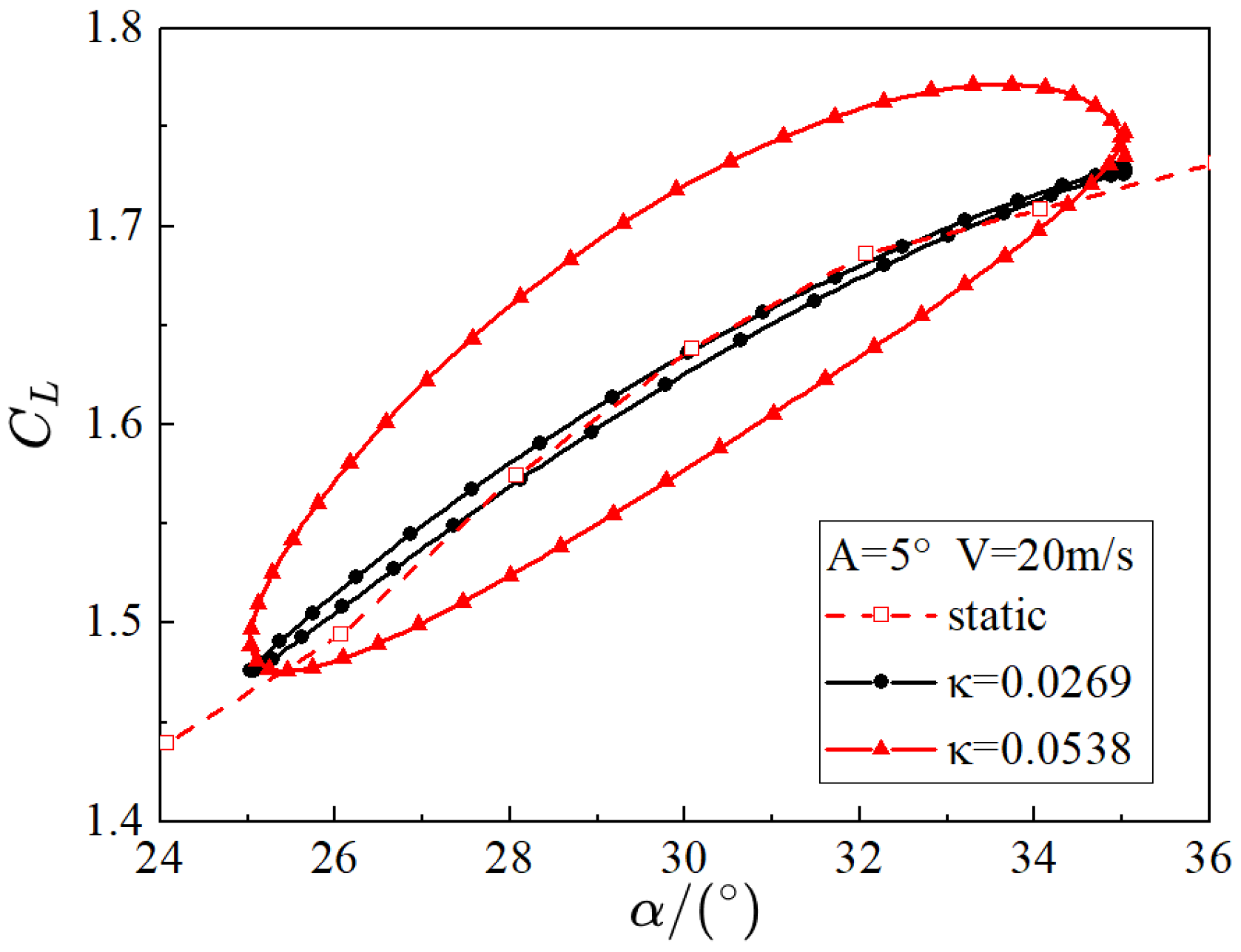
Pitch oscillation experiments are conducted on the WDPR-8. In the pitch oscillations, the reduced frequency is defined as:
where the mean aerodynamic chord length of the aircraft model is 0.2522 m, the free-stream velocity in the test section is 20 m/s, and the Reynolds number is approximately . With an oscillation amplitude of 5°, the reduced frequency is calculated to be 0.0269 and 0.0538, corresponding to oscillation frequencies of 0.34 Hz and 0.68 Hz, respectively. The experiments were conducted at initial angles of attack ranging from −10° to 30°, with increments of 10°. Figure 6 shows the results of single-degree-of-freedom pitch oscillation tests at various reduced frequencies.
Furthermore, high-angles-of-attack pull-up tests, frequency sweep tests, amplitude sweep tests, and multi-degree of freedom oscillation tests were also conducted. Figure 7 shows the pull-up of angle of attack for the aircraft model with WDPR-8 from 50° to 80°.
To train and validate the prediction performance at high angles of attack of the proposed model, additional training data from wind tunnel experiments performed by the Aviation Industry Corporation of China Aerodynamics Research Institute were also utilized [34]. The dataset includes results of the same aircraft model with both static experiments, the angle of attack ranging from 0° to 80°, and dynamic wind tunnel experiments, which were based on large amplitude pitch oscillations and can be described by the Equation (12). Typical dynamic experiments include the oscillation amplitude of 40° at various oscillation frequencies, including 0.2, 0.4, 0.6, and 0.8 Hz.
Data derived from the above experiments were divided into two subsets. Training sets were used to adjust the weights and parameters of the model. Test sets were used to evaluate the model’s interpolation and extrapolation prediction performance.
The performance of the model is evaluated using the mean squared error. A smaller MSE indicates better performance.
3.1.2. Model Training
In this experiment, the flight state vector is chosen to consist of the angles of attack , pitch rate , oscillation frequency , and oscillation amplitude , denoted as . The pitching moment coefficient , as an example, is used as the model output, while other aerodynamic coefficients are not additionally displayed.
Figure 8 presents a comparison of the training curves for models with and without a feature standardization layer after 100 rounds of training. It is evident from Table 1 that data standardization improves both the training efficiency and prediction accuracy of the model. As the training results (Figure 9) show, the outputs of the WFFM match quite well with the experimental data, which exhibits the powerful non-linear fitting capability of the WFFM.
3.1.3. Model Testing
The performance of the models in the interpolation test is shown in Figure 10. The MSE of the results are shown in Table 2. In addition to the WFFM, the state-space (SS) model, LSTM model, and feature fusion model (FFM, without the feature weighting layer) were also employed for comparison. The results show that the pitch moment predictions from all models match with the experimental data. The results presented in Table 2 show that the black-box model was better than the state-space model in the interpolation test. Furthermore, by combining the state-space model with the black-box model, the results of the FFM and WFFM are improved in prediction accuracy. It is also observed that the introduction of the feature weighting layer leads to more accurate results for the WFFM.
The models’ prediction results and the MSE of results in the extrapolation test are shown in Figure 11 and Table 3, respectively. It can be observed that the overall error for extrapolation is higher than for interpolation. The MSE of the SS model was slightly lower than that of the LSTM model, which is contrary to the results of the interpolation test. This is because a neural network cannot map the function in regions of the variable space where no training data is available. The FFM and WFFM obtain physical mechanisms by introducing a state-space model, which enables the models to obtain higher-precision prediction results. Compared to the FFM, the WFFM exhibits an accuracy improvement of up to 50%, indicating that feature fusion effectively reduces additional errors.
In summary, the results demonstrated the outstanding performance of the WFFM in predicting unsteady aerodynamic loads at high angles of attack. Within the framework of combining the state-space model with a neural network, the FFM and the WFFM strengthen the capabilities of extrapolation. The introduction of the feature weighting layer effectively reduces the additional error from the state-space model and improves the prediction accuracy. This method demonstrates its potential for practical application in aircraft design and control.
3.2. Flight Simulation Tests
3.2.1. Flight Simulation
Due to the lack of real flight data, simulated flight data is used for training and validating the proposed aerodynamic models. In this section, a non-linear F-16 flight dynamics model is used. This plant can simulate the response of F-16 aircraft (Lockheed Martin, Bethesda, MD, USA) using the aerodynamic model and aerodynamic data as described by a NASA report [35]. The structure of the flight simulation model is shown in Figure 12. Different control signals are input into the F-16 dynamic equations, which are coupled with various aerodynamic models. The resulting flight states are then compared to validate the accuracy of the aerodynamic models. The dynamic equations of this aircraft in the body-fixed reference axes can be expressed as:
Forces:
Moments:
where , , and are the force coefficients on the , , and axes, respectively. , , and are the rolling, pitching, and yawing moment coefficients, respectively. The force and moment coefficients, derived from experimental data performed in a NASA Langley wind tunnel, are found by interpolating the data points for a given angle of attack, sideslip, and elevator deflection. Then, the Euler angles were computed by using quaternions to allow continuity of attitude motions. Auxiliary equations included:
where and are the normal acceleration and lateral acceleration.
To start the simulation process, it is essential to find steady-state flight conditions for the force and moment equilibriums. Since this paper focuses on longitudinal dynamic characteristics, the lateral-directional motion is considered to be de-coupled. We trim the F-16 for steady level flight with velocity and altitude . After trimming, the angle of attack , pitch angle , elevator deflection , and throttle setting are obtained. The trim state and control inputs are presented in Table 4.
To train and evaluate the aerodynamic models, various control commands are chosen to generate simulated data. For the performance comparison, the coefficient of determination, denoted as , is used as the evaluation criterion. When evaluating the goodness-of-fit of predicted values against actual values, a higher value indicates better predictive performance.
where is the total number of samples, represents the actual values, is the mean of the actual values, and is the predicted values.
3.2.2. Training Results for Sinusoidal Input
In the flight simulation, the flight states variables of aerodynamic models are selected as angle of attack , pitch rate , pitch angle , flight speed , and elevator deflection , denoted as , and the output is the vector of aerodynamic coefficients .
To obtain the flight states such as angle of attack and pitch angle, the aerodynamic model was coupled with the flight dynamics model. By using various combinations of elevator inputs, we can obtain aerodynamic loads for different maneuvers.
For aerodynamic modeling, sinusoidal control command on the elevators is designed to generate training data. The elevator input frequencies for the training set were selected as 0.1, 0.2, 0.3, 0.4, and 0.5 Hz, and the amplitudes were chosen as 1, 2, 3, 4, and 5 degrees. These different combinations of amplitudes and frequencies resulted in a total of 25 experiments. The simulation duration was set to 15 s. Figure 13 shows a sinusoidal control input with an amplitude of 3° and a frequency of 0.3 Hz. The WFFM’s predictions, as shown in Figure 14, matched well with the F-16 model’s response.
3.2.3. Testing Results for Sweep Input
To thoroughly assess the predictive capability of the aerodynamic models obtained in Section 3.2.2, two sets of sweep signal with variable frequency and variable amplitude are designed as control inputs, represented as:
where the frequency variation is given by:
and the amplitude variation for the first set of experiments is given by:
and the amplitude variation for the second set of experiments is given by:
The maximum frequency is set to 0.6 Hz, and the maximum amplitude is set to 6°. The simulation duration is 10 s. Figure 15 displays the frequency and amplitude of the sweep control input variation over time, exhibiting a characteristic S″-shaped curve. Figure 16 presents the sweep control input history.
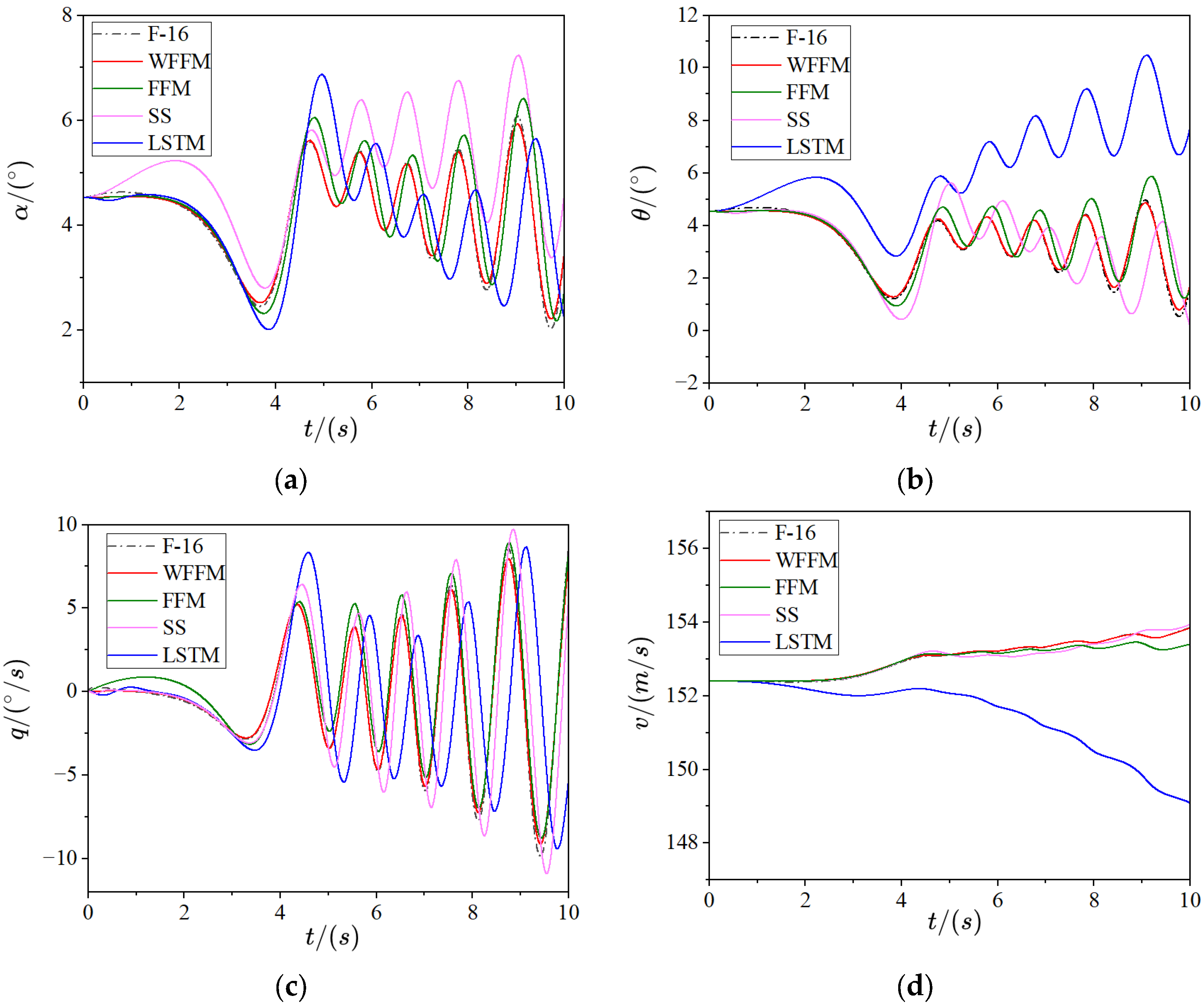
Similarly, the aerodynamic model is incorporated into the flight dynamics models to observe the flight state variables. As shown in Table 5, the values for both the state-space model and LSTM model are less than 0.9, indicating a relatively large error. As shown in Figure 17 and Figure 18, the outputs of the LSTM model deviate significantly from the real flight states, which shows the limits of the black-box model to accurately predict aerodynamics in flight simulation. The FFM shows minor differences in flight states compared to the real values, and its values are greater than 0.9. The WFFM outputs values exceeding 0.99 in both simulation tests. The comparisons between the WFFM and F-16 model show good agreements in all states.
3.2.4. Testing Results for Doublet Input
To assess the generality of the models, a 4-deg doublet control input, as shown in Figure 19, is applied to the models established in Section 3.2.2. Since the models were trained under sinusoidal inputs, doublet inputs can further evaluate the adaptability and practicality of the established models.
From the simulation results shown in Figure 20 and Table 6, it can be observed that the FFM and WFFM exhibit higher precision compared to the SS and LSTM models. This suggests that embedding the physical model into the black-box model can effectively improve both the predictive accuracy and the robustness of the neural network model. However, the FFM still cannot perfectly fit the flight states of the F-16 model. Figure 20 shows that all the state curves from the WFFM match with the F-16 model fairly well. Table 6 shows that the WFFM maintains an value exceeding 0.99. It can be concluded that the results of the WFFM are not only more precise but also more general in comparison with the FFM.
3.2.5. Testing Results for High-Angle-of-Attack Maneuvers
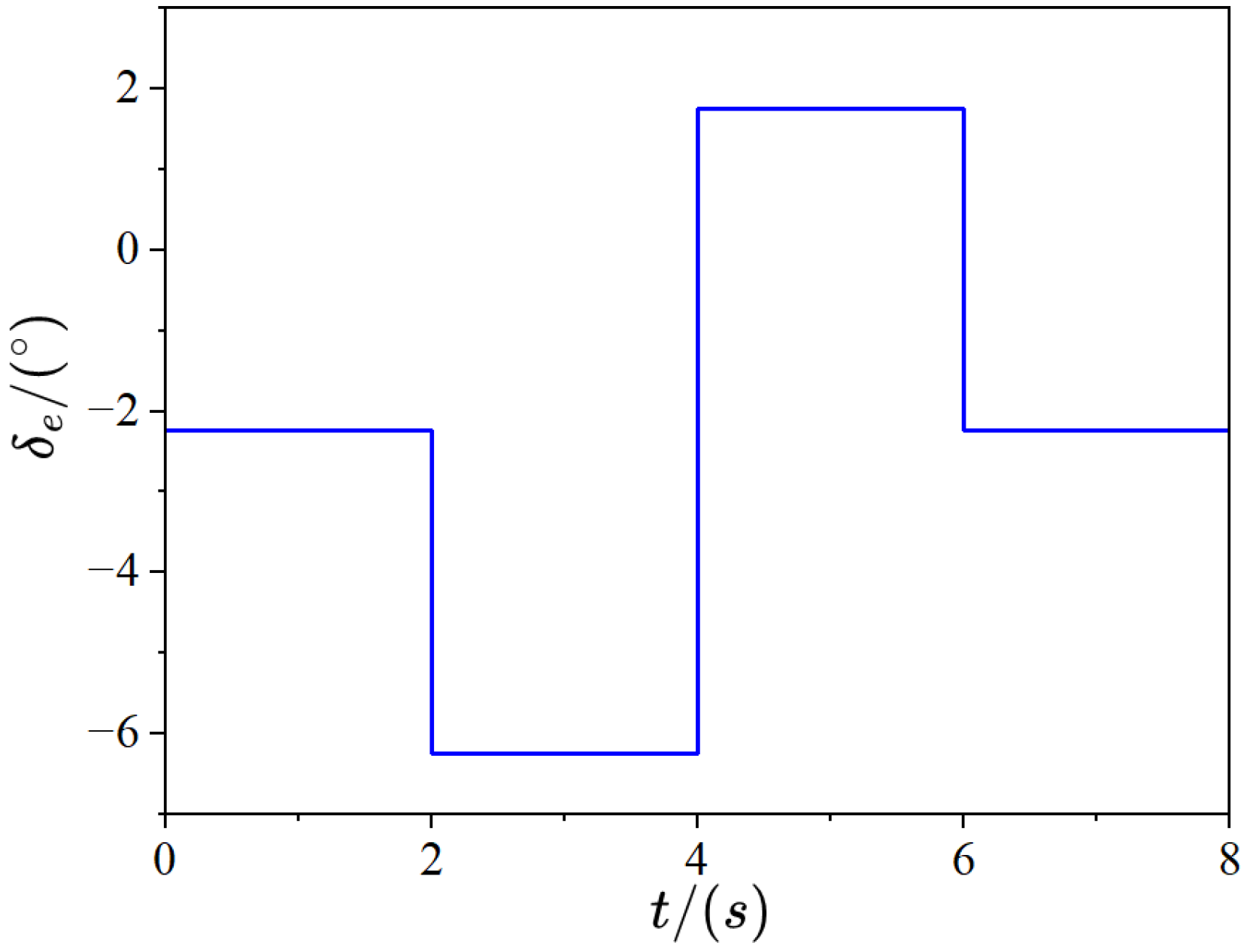
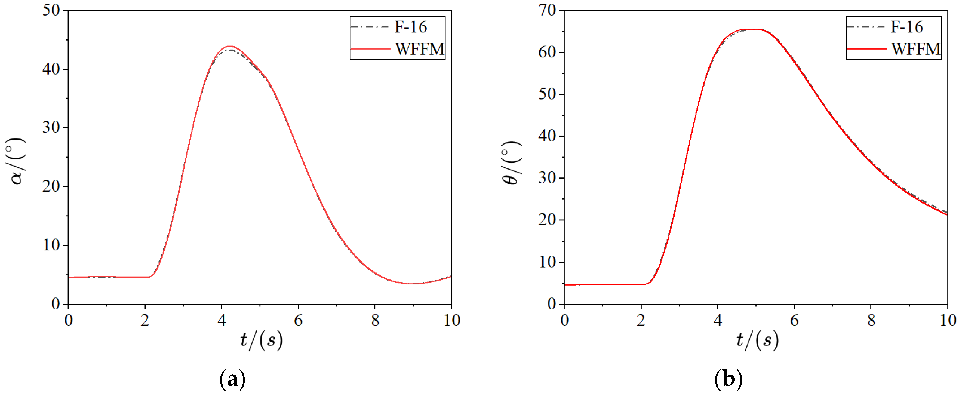
In this section, the aerodynamic model’s accuracy at a high angle of attack was tested. By rapidly increasing the elevator deflection angle, the aircraft achieved a swift increase in both angle of attack and pitch angle within a short duration. During the maneuver, the aircraft was at a high angle of attack, resulting in significant changes in airflow over the aircraft’s surface, including flow separation, vortex formation, and complex vortex interactions. These effects lead to nonlinear changes in aerodynamic forces and moments, making them challenging to accurately predict with simple aerodynamic models.
In this test, the aerodynamic model obtained in Section 3.2.2 was further trained with elevator deflection increments of 5°, 8°, 10°, and 15°, and tested with a deflection increment of 13°. The test input, as shown in Figure 21, involved a step signal where the elevator angle rapidly deflected from a trim angle of −2.24° to −15.24°. At this point, the pitch angle and angle of attack, as illustrated in Figure 22, rapidly increased to 65° and 43°, respectively. The value of the WFFM is 0.9912, which demonstrates that the WFFM can accurately predict the aerodynamics of the aircraft during high-angle-of-attack maneuvers.
4. Conclusions
In this paper, a novel proposed aerodynamic model called the weighted feature fusion model was implemented. By comparing the results of the state-space model, LSTM model, FFM, and WFFM in high-angles-of-attack aerodynamic prediction and flight simulation tests, the main conclusions of this study are as follows:
- (1)
- Compared to the black-box model, embedding the physics model with explicit physical meaning into the neural network improves both the interpolation and extrapolation capability of the model.
- (2)
- Compared to the FFM, further consideration of limiting the error of the physical model by introducing a weighted coefficient layer can improve the accuracy of aerodynamic prediction and simulation accuracy.
- (3)
- In flight simulation, the flight states based on the WFFM’s outputs are very close to the F-16 model’s, indicating that it can replace existing aerodynamic models.
Author Contributions
Conceptualization, W.D. and X.W.; methodology, W.D.; software, W.D.; validation, W.D.; formal analysis, W.D. and C.C.; investigation, W.D.; resources, X.W., Q.L. and L.Z.; data curation, W.D.; writing—original draft preparation, W.D.; writing—review and editing, X.W., Q.L., C.C. and L.Z.; visualization, W.D.; supervision, X.W. and Q.L.; project administration, X.W. and Q.L.; funding acquisition, X.W. and L.Z. All authors have read and agreed to the published version of the manuscript.
Funding
This research was supported by the National Natural Science Foundation of China under Grant Nos. 12172315, 12072304, 11702232, the Fujian Provincial Natural Science Foundation of China (2021J01050), and the National Key Laboratory of Aerodynamics (61422010103).
Data Availability Statement
The data are contained within the article.
Conflicts of Interest
The authors declare no conflicts of interest.
References
- Bryan, G.H.; Williams, W.E. The Longitudinal Stability of Aerial Gliders. Proc. R. Soc. Lond. 1904, 73, 100–116. [Google Scholar] [CrossRef]
- Lin, G.-F.; Lan, C.; Brandon, J. A generalized dynamic aerodynamic coefficient model for flight dynamics applications. In Proceedings of the 22nd Atmospheric Flight Mechanics Conference, New Orleans, LA, USA, 11–13 August 1997. [Google Scholar]
- Mi, B.-G.; Zhan, H.; Lu, S.-S. An extended unsteady aerodynamic model at high angles of attack. Aerosp. Sci. Technol. 2018, 77, 788–801. [Google Scholar] [CrossRef]
- Hao, D.; Zhang, L.; Yu, J.; Mao, D. Modeling of unsteady aerodynamic characteristics at high angles of attack. Proc. Inst. Mech. Eng. Part G J. Aerosp. Eng. 2018, 233, 2291–2301. [Google Scholar] [CrossRef]
- Wang, X.; Kou, J.; Zhang, W. Unsteady aerodynamic modeling based on fuzzy scalar radial basis function neural networks. Proc. Inst. Mech. Eng. Part G J. Aerosp. Eng. 2019, 233, 5107–5121. [Google Scholar] [CrossRef]
- Ghoreyshi, M.; Cummings, R. Aerodynamics Modeling of A Maneuvering Aircraft Using Indicial Functions. In Proceedings of the 50th AIAA Aerospace Sciences Meeting including the New Horizons Forum and Aerospace Exposition, Nashville, TN, USA, 9–12 January 2012. [Google Scholar]
- Chen, S.; Gao, Z.; Zhu, X.; Du, Y.; Pang, C. Unstable unsteady aerodynamic modeling based on least squares support vector machines with general excitation. Chin. J. Aeronaut. 2020, 33, 2499–2509. [Google Scholar] [CrossRef]
- Wang, Q.; Qian, W.; He, K. Unsteady aerodynamic modeling at high angles of attack using support vector machines. Chin. J. Aeronaut. 2015, 28, 659–668. [Google Scholar] [CrossRef]
- Yetkin, S.; Abuhanieh, S.; Yigit, S. Investigation on the abilities of different artificial intelligence methods to predict the aerodynamic coefficients. Expert Syst. Appl. 2023, 237, 121324. [Google Scholar] [CrossRef]
- Xiong, F.; Zhang, L.; Hu, X.; Ren, C. A point cloud deep neural network metamodel method for aerodynamic prediction. Chin. J. Aeronaut. 2023, 36, 92–103. [Google Scholar] [CrossRef]
- Ignatyev, D.I.; Khrabrov, A.N. Neural network modeling of unsteady aerodynamic characteristics at high angles of attack. Aerosp. Sci. Technol. 2015, 41, 106–115. [Google Scholar] [CrossRef]
- Wu, H.; Liu, X.; An, W.; Lyu, H. A generative deep learning framework for airfoil flow field prediction with sparse data. Chin. J. Aeronaut. 2022, 35, 470–484. [Google Scholar] [CrossRef]
- Li, W.; Laima, S.; Jin, X.; Yuan, W.; Li, H. A novel long short-term memory neural-network-based self-excited force model of limit cycle oscillations of nonlinear flutter for various aerodynamic configurations. Nonlinear Dyn. 2020, 100, 2071–2087. [Google Scholar] [CrossRef]
- Li, K.; Kou, J.; Zhang, W. Deep neural network for unsteady aerodynamic and aeroelastic modeling across multiple Mach numbers. Nonlinear Dyn. 2019, 96, 2157–2177. [Google Scholar] [CrossRef]
- Wang, Q.; He, K.-F.; Qian, W.-Q.; Zhang, T.-J.; Cheng, Y.-Q.; Wu, K.-Y. Unsteady aerodynamics modeling for flight dynamics application. Acta Mech. Sin. 2012, 28, 14–23. [Google Scholar] [CrossRef]
- Chen, H.; He, L.; Qian, W.; Wang, S. Multiple Aerodynamic Coefficient Prediction of Airfoils Using a Convolutional Neural Network. Symmetry 2020, 12, 544. [Google Scholar] [CrossRef]
- Zuo, K.; Ye, Z.; Zhang, W.; Yuan, X.; Zhu, L. Fast aerodynamics prediction of laminar airfoils based on deep attention network. Phys. Fluids 2023, 35, 037127. [Google Scholar] [CrossRef]
- Faroughi, S.A.; Pawar, N.; Fernandes, C.; Raissi, M.; Das, S.; Kalantari, N.K.; Mahjour, S.K. Physics-Guided, Physics-Informed, and Physics-Encoded Neural Networks in Scientific Computing. arXiv 2023, arXiv:2211.07377. [Google Scholar]
- Raissi, M.; Perdikaris, P.; Karniadakis, G.E. Physics-informed neural networks: A deep learning framework for solving forward and inverse problems involving nonlinear partial differential equations. J. Comput. Phys. 2019, 378, 686–707. [Google Scholar] [CrossRef]
- Zhao, T.; Chen, G.; Wang, X.; Yong, E.; Qian, W. Aerodynamic modeling using an end-to-end learning attitude dynamics network for flight control. Acta Mech. Sin. 2022, 37, 1799–1811. [Google Scholar] [CrossRef]
- Kangli, L.; Zhiwei, S.; Junquan, F.; Weilin, T.S. Comparative analysis of three machine learning methods for unsteady aerodynamic modeling. Flight Dyn. 2023, 41, 33–39. [Google Scholar]
- Kou, J.; Zhang, W. Data-driven modeling for unsteady aerodynamics and aeroelasticity. Prog. Aerosp. Sci. 2021, 125, 100725. [Google Scholar] [CrossRef]
- Wang, X.; Kou, J.; Zhang, W.; Liu, Z. Incorporating Physical Models for Dynamic Stall Prediction Based on Machine Learning. AIAA J. 2022, 60, 4428–4439. [Google Scholar] [CrossRef]
- Huailu, L.; Xu, W.; Xiao, W. Aerodynamic modeling and flight simulation of maneuverable flight at high angle of attack. Acta Aeronaut. Et Astronaut. Sin. 2023, 44, 128410. [Google Scholar]
- Zhang, W.; Peng, X.; Kou, J.; Wang, X. Heterogeneous data-driven aerodynamic modeling based on physical feature embedding. Chin. J. Aeronaut. 2023, 37, 1–6. [Google Scholar] [CrossRef]
- Goman, M.; Khrabrov, A. State-space representation of aerodynamic characteristics of an aircraft at high angles of attack. J. Aircr. 1994, 31, 1109–1115. [Google Scholar] [CrossRef]
- Bryan, G.H. Stability in Aviation: An Introduction to Dynamical Stability as Applied to the Motions of Aeroplanes; Macmillan and Co., Ltd.: London, UK, 1911. [Google Scholar]
- Ioffe, S.; Szegedy, C. Batch Normalization: Accelerating Deep Network Training by Reducing Internal Covariate Shift. Proc. Mach. Learn. Res. 2015, 37, 448–456. [Google Scholar]
- LeCun, Y.; Touresky, D.; Hinton, G.; Sejnowski, T. A theoretical framework for back-propagation. In Proceedings of the 1988 Connectionist Models Summer School, Pittsburgh, PA, USA, 17–26 June 1988; pp. 21–28. [Google Scholar]
- Xiao, Y.; Lin, Q.; Zheng, Y.; Bin, L. Model Aerodynamic Tests with a Wire-driven Parallel Suspension System in Low-speed Wind Tunnel. Chin. J. Aeronaut. 2010, 23, 393–400. [Google Scholar]
- Wang, X.G.; Lin, Q. Progress in wire-driven parallel suspension technologies in wind tunnel tests. Acta Aeronaut. Et Astronaut. Sin. 2018, 39, 6–25. [Google Scholar]
- Pan, J.; Lin, Q.; Wu, H.; Zhou, F.; Wang, X. Comparative experimental study on wind tunnel based on WDPR-8 and machetes tail support. J. Beijing Univ. Aeronaut. Astronaut. 2021, 47, 1038–1048. [Google Scholar]
- Wang, X.; Shen, C.; Jiang, H.; Lin, Q.; Ji, Y. Optimal Design and Verifications of Cable-Suspension Mechanism for High-Angle-of-Attack Unsteady Tests. J. Aircr. 2023, 60, 2017–2023. [Google Scholar] [CrossRef]
- Liu, C.M.; Zhao, Z.J.; Bu, C.; Wang, J.F.; Mu, W.Q. Double degree-of-freedom large amplitude oscillation test technology in low speed wind tunnel. Acta Aeronaut. Astronaut. Sin. 2016, 37, 2417–2425. [Google Scholar]
- Nguyen, L.T.; Ogburn, M.E.; Gilbert, W.P.; Kibler, K.S.; Brown, P.W.; Deal, P.L. Simulator Study of Stall/Post-Stall Characteristics of a Fighter Airplane with Relaxed Longitudinal Static Stability; National Aeronautics and Space Administration: Washington, DC, USA, 1979. [Google Scholar]
Figure 1.
A typical neural network used to predict aerodynamic loads.

Figure 2.
LSTM uses flight state history data to predict aerodynamic loads.

Figure 3.
Architecture of WFFM.

Figure 4.
WDPR-8 in the wind tunnel.

Figure 5.
Lift coefficients with WDPR-8 and tail support.

Figure 6.
Lift coefficients at various reduced frequencies.

Figure 7.
Pull-up maneuver of aircraft model with WDPR-8.

Figure 8.
Comparison of training progress with and without standardization.

Figure 9.
The prediction of WFFM compared with the experimental data in the training set: (a) static; (b) f = 0.2 Hz; (c) f = 0.6 Hz.
Figure 9.
The prediction of WFFM compared with the experimental data in the training set: (a) static; (b) f = 0.2 Hz; (c) f = 0.6 Hz.

Figure 10.
Comparison of prediction results of WFFM, FFM, SS, and LSTM for interpolation test.

Figure 11.
Comparison of prediction results of WFFM, FFM, SS, and LSTM for extrapolation test.

Figure 12.
Structure of the flight simulation.

Figure 13.
Sinusoidal control input with A = 3° and f = 0.3 Hz.

Figure 14.
Response of WFFM and F-16 model to the sinusoidal input with A = 3° and f = 0.3 Hz: (a) angle of attack; (b) pitch angle; (c) pitch rate; (d) velocity.
Figure 14.
Response of WFFM and F-16 model to the sinusoidal input with A = 3° and f = 0.3 Hz: (a) angle of attack; (b) pitch angle; (c) pitch rate; (d) velocity.

Figure 15.
Frequency and amplitude of sweep control input variation over time: (a) frequency; (b) amplitude.
Figure 15.
Frequency and amplitude of sweep control input variation over time: (a) frequency; (b) amplitude.

Figure 16.
Sweep control input: (a) set 1; (b) set 2.

Figure 17.
Response of WFFM, FFM, SS, and LSTM to the first sweep input: (a) angle of attack; (b) pitch angle; (c) pitch rate; (d) velocity.
Figure 17.
Response of WFFM, FFM, SS, and LSTM to the first sweep input: (a) angle of attack; (b) pitch angle; (c) pitch rate; (d) velocity.

Figure 18.
Response of WFFM, FFM, SS, and LSTM to the second sweep input: (a) angle of attack; (b) pitch angle; (c) pitch rate; (d) velocity.
Figure 18.
Response of WFFM, FFM, SS, and LSTM to the second sweep input: (a) angle of attack; (b) pitch angle; (c) pitch rate; (d) velocity.

Figure 19.
The 4-deg doublet control input.

Figure 20.
Response of WFFM, FFM, SS, and LSTM to the 4-deg doublet input: (a) angle of attack; (b) pitch angle; (c) pitch rate; (d) velocity.
Figure 20.
Response of WFFM, FFM, SS, and LSTM to the 4-deg doublet input: (a) angle of attack; (b) pitch angle; (c) pitch rate; (d) velocity.

Figure 21.
Step control input and elevator deflection with 13° increment.

Figure 22.
Response of WFFM to the high-angle-of-attack maneuver: (a) angle of attack; (b) pitch angle.
Figure 22.
Response of WFFM to the high-angle-of-attack maneuver: (a) angle of attack; (b) pitch angle.


Table 1.
The MSE of WFFM for training sets.
| Frequency | Static | 0.2 Hz | 0.6 Hz |
|---|---|---|---|
| MSE |
Table 2.
The MSE of WFFM for interpolation test.
| WFFM | FFM | LSTM | SS | |
|---|---|---|---|---|
| MSE |
Table 3.
The MSE of WFFM for extrapolation test.
| WFFM | FFM | LSTM | SS | |
|---|---|---|---|---|
| MSE |
Table 4.
F-16 trim condition.
| Parameter | Value | Unit |
|---|---|---|
| 4572 | m | |
| 152 | m/s | |
| 4.53 | deg | |
| 4.53 | deg | |
| −2.24 | deg | |
| 0.46 | - |
Table 5.
The coefficient of determination for sweep input.
| Set 1 | Set 2 | |||||||
| WFFM | 0.9995 | 0.9997 | 0.9981 | 0.9999 | 0.9982 | 0.9986 | 0.9984 | 0.9996 |
| FFM | 0.9793 | 0.9862 | 0.9607 | 0.9977 | 0.9021 | 0.8197 | 0.9861 | 0.9596 |
| SS | 0.9738 | 0.9574 | 0.9629 | 0.9989 | 0.8104 | 0.6463 | 0.9726 | 0.9543 |
| LSTM | 0.7666 | 0.8578 | 0.7212 | 0.9637 | 0.7979 | 0.6805 | 0.8875 | 0.7045 |
Table 6.
The coefficient of determination for doublet input.
| Average | |||||
| WFFM | 0.9997 | 0.9997 | 0.9995 | 0.9999 | 0.9997 |
| FFM | 0.9928 | 0.9790 | 0.9879 | 0.9983 | 0.9895 |
| SS | 0.9661 | 0.9589 | 0.9359 | 0.9936 | 0.9636 |
| LSTM | 0.8551 | 0.8252 | 0.8186 | 0.9973 | 0.8741 |
Disclaimer/Publisher’s Note: The statements, opinions and data contained in all publications are solely those of the individual author(s) and contributor(s) and not of MDPI and/or the editor(s). MDPI and/or the editor(s) disclaim responsibility for any injury to people or property resulting from any ideas, methods, instructions or products referred to in the content. |
© 2024 by the authors. Licensee MDPI, Basel, Switzerland. This article is an open access article distributed under the terms and conditions of the Creative Commons Attribution (CC BY) license (https://creativecommons.org/licenses/by/4.0/).
Share and Cite
MDPI and ACS Style
Dong, W.; Wang, X.; Lin, Q.; Cheng, C.; Zhu, L. A Weighted Feature Fusion Model for Unsteady Aerodynamic Modeling at High Angles of Attack. Aerospace 2024, 11, 339. https://doi.org/10.3390/aerospace11050339
AMA Style
Dong W, Wang X, Lin Q, Cheng C, Zhu L. A Weighted Feature Fusion Model for Unsteady Aerodynamic Modeling at High Angles of Attack. Aerospace. 2024; 11(5):339. https://doi.org/10.3390/aerospace11050339
Chicago/Turabian StyleDong, Wenzhao, Xiaoguang Wang, Qi Lin, Chuan Cheng, and Liangcong Zhu. 2024. "A Weighted Feature Fusion Model for Unsteady Aerodynamic Modeling at High Angles of Attack" Aerospace 11, no. 5: 339. https://doi.org/10.3390/aerospace11050339
Note that from the first issue of 2016, this journal uses article numbers instead of page numbers. See further details here.