Article

Physical Modeling and Simulation of Reusable Rockets for GNC Verification and Validation †

by
Stefano Farì
1,*,
Marco Sagliano
1,
José Alfredo Macés Hernández
1,
Anton Schneider
2,
Ansgar Heidecker
1,
Markus Schlotterer
1 and
Svenja Woicke
1
1
German Aerospace Center (DLR), Department of Navigation and Control Systems, Institute of Space Systems, Robert-Hooke-Str. 7, 28359 Bremen, Germany
2
German Aerospace Center (DLR), Department of Landing and Exploration Technology, Institute of Space Systems, Robert-Hooke-Str. 7, 28359 Bremen, Germany
*
Author to whom correspondence should be addressed.
This paper is an extension of “The Vertical Landing Vehicles Library (VLVLib): A Modelica-based approach to high-fidelity simulation and verification of GNC systems for reusable rockets” presented at the 73rd International Astronautical Congress (IAC), Paris, France, 18–22 September 2022.
Aerospace 2024, 11(5), 337; https://doi.org/10.3390/aerospace11050337
Submission received: 24 November 2023 / Revised: 18 April 2024 / Accepted: 22 April 2024 / Published: 24 April 2024
(This article belongs to the Special Issue GNC for the Moon, Mars, and Beyond)

Abstract

:
Reusable rockets must rely on well-designed Guidance, Navigation and Control (GNC) algorithms. Because they are tested and verified in closed-loop, high-fidelity simulators, emphasizing the strategy to achieve such advanced models is of paramount importance. A wide spectrum of complex dynamic behaviors and their cross-couplings must be captured to achieve sufficiently representative simulations, hence a better assessment of the GNC performance and robustness. This paper focuses on of the main aspects related to the physical (acausal) modeling of reusable rockets, and the integration of these models into a suitable simulation framework oriented towards GNC Validation and Verification (V&V). Firstly, the modeling challenges and the need for physical multibody models are explained. Then, the Vertical Landing Vehicles Library (VLVLib), a Modelica-based library for the physical modeling and simulation of reusable rocket dynamics, is introduced. The VLVLib is built on specific principles that enable quick adaptations to vehicle changes and the introduction of new features during the design process, thereby enhancing project efficiency and reducing costs. Throughout the paper, we explain how these features allow for the rapid development of complex vehicle simulation models by adjusting the selected dynamic effects or changing their fidelity levels. Since the GNC algorithms are normally tested in Simulink®, we show how simulation models with a desired fidelity level can be developed, embedded and simulated within the Simulink® environment. Secondly, this work details the modeling aspects of four relevant vehicle dynamics: propellant sloshing, Thrust Vector Control (TVC), landing legs deployment and touchdown. The CALLISTO reusable rocket is taken as study case: representative simulation results are shown and analyzed to highlight the impact of the higher-fidelity models in comparison with a rigid-body model assumption.

1. Introduction

The beginning of the rocket reusability era, formally marked on 21 December 2015 by SpaceX [1], stimulated efforts all around the world to design and industrialize new reliable space transportation systems. This effect is not only noticeable among other private companies like Blue Origin and Rocket Lab [2], but also at research and governmental levels. In Europe, several technology demonstrators and commercial launchers are being developed, like CALLISTO [3,4], Themis [5] and Miura 5 [6]; on the other hand, the Ariane Next reusable launcher development program aims at achieving reusability in a commercial context [7]. The interest towards reusable rockets goes well beyond the simple use for terrestrial applications, because they are expected to be one of the cornerstones in the next phase of human space exploration and exploitation.
This paper tackles the important, though oftentimes underestimated, aspect of the Validation and Verification (V&V) activities of the vehicle’s Guidance, Navigation and Control (GNC) system, which is crucial to maximize the mission success likelihood by satisfying a set of strict requirements, while taking into account the coupling between various subsystems and effects such as propulsion, aerodynamics, and structure. For Reusable Launch Vehicles (RLVs), this is even more relevant due to the presence of several actuation systems like landing legs, aerodynamic fins and the Reaction Control System (RCS). The synthesis models used for GNC design are typically built in a simplified manner and neglect some dynamics, especially when adopting linear synthesis and analysis techniques, with the implicit assumption that their impact on the performance and the robustness of the overall system is negligible as well. This assumption cannot be taken for granted and, therefore, the current models in use cannot be considered representative benchmarks by default. The objective is to have a more representative assessment of the degradation in performance and robustness, especially in the early development stages, when experimental tests may not be possible. However, the setup of such a framework is a time-consuming activity: since GNC design and V&V are iterative processes (Figure 1), the reusability of models must be maximized and the simulation model fidelity levels quickly adapted. While early in the design cycle simplicity and speed are prioritized, as development progresses incorporating advanced physical simulation models and hardware test results to enhance model fidelity becomes crucial in detecting flaws and improving the GNC algorithms [8]. Consequently, frameworks oriented to a more efficient adaptation to new models, new mission designs, or even new vehicles are needed. Note that ‘physical modeling’ refers to the use of mathematical equations to simulate the dynamics of cyber-physical systems, capturing both their physical and computational aspects.
The development of simulation models for GNC testing often relies heavily on the use of Simulink®, since is convenient for rapid prototyping and testing of dynamic models. Simulink® is a ‘causal’ (or ‘block-oriented’) modeling environment. Causal models define the relation between different dynamical elements solely by the output of one block being fed into the input of another block. This architecture operates on a causal modeling principle, where the output from one block feeds directly into the next. This sequential data flow is logical, but limited, as it struggles with complex systems where the energy flow is not strictly one-way. To implement simulation models in Simulink®, users often have to manually write (or re-work) their dynamic equations to establish an input–output relationship first. This (re-)formatting detaches the model from its real-world counterpart, makes component reuse difficult, and necessitates further significant rework if the system configuration changes. This is particularly problematic for RLV simulations, which may require various levels of detail or the addition/removal of dynamics, depending on the current project phase or needs. In Simulink®, it is also overly complex or impossible to handle models involving algebraic constraints. Furthermore, it is not easy to vary the fidelity level of the different sub-components, or to model interactions between different types of physical processes.
On the other hand, acausal modeling, enabled by Simscape® and the Modelica language, allow for an energy-oriented approach, more intuitive for representing complex physical systems. These tools employ specialized connectors that define component interactions using the underlying physical equations without preset directions of computational causality. This methodology aligns closely with the energy flows and the dynamics inherent in complex physical systems. In this work, we choose to employ the Modelica modeling language; RLV models greatly benefit from their ability to build detailed, energy-conservative multibody dynamics through these connectors. As such, a more accurate representation of the mechanical interactions within the rocket is possible, improving the fidelity and utility of the simulation. The Modelica language is also open-source and object-oriented; this contributes to the implementation of efficient, scalable and adaptable simulation models, making it suitable for the complexity of reusable rockets.
An example of Simscape®-based reusable rocket modeling can be found in [9]. On the other hand, Modelica has already been used in several space-related contexts, like vehicle re-entry scenarios via a guided parafoil, lunar landing missions, or modeling rocket fuel slosh dynamics [10,11,12]. There exist several flight dynamics libraries, such as the DLR Flight Dynamics Library [13] or the Space Flight Dynamic library [14]. In addition, there were applications to launch vehicle dynamics, control and trajectory optimization [15], or stage separation [16]. The language, therefore, fits well with the development of high-fidelity RLV physical models. However, the available libraries are oftentimes not specifically tailored to meet the V&V needs from the GNC point of view and state-of-practice. In fact, they tend to centralize the modeling and simulation processes within the chosen Modelica-based software, thus forcing the abandonment of pre-existing and already tested Matlab-Simulink® functions and setups. For these reasons, the Vertical Landing Vehicles Library (VLVLib) has been specifically developed over the last years to meet these more specific demands [17].
This work covers several relevant modeling and simulation aspects from the perspective described above: Section 2 describes the most relevant dynamics to be captured when modeling reusable rockets. From here, a more detailed explanation of the benefits of acausal (physical) modeling is given in Section 3. Since the Modelica language is employed, we explain how to build up a Simulink®-based simulation framework with co-simulated Modelica models [18]. In this work, emphasis is placed on propellant slosh dynamics, Thrust Vector Control (TVC), landing leg deployment and touchdown dynamics, which are well-known to be potentially hazardous without a robust GNC system. Accordingly, Section 4, Section 5, Section 6 and Section 7 detail their modeling, respectively. CALLISTO RLV demonstrator is taken as study case: the impact of the high-fidelity models is, in this context, compared with a benchmark causal rigid-body vehicle model. We show and analyze representative simulation results in Section 8. Finally, we draw some conclusions about this work in Section 9.

2. Modeling Challenges and Simulation Framework

The modeling of reusable rockets is one of the most challenging tasks for control engineers designing the vehicle GNC system. This is due to:
  • The multidisciplinary nature of the involved dynamics;
  • The difference in the vehicle operational regimes during different test flights;
  • The difficulty in quickly incorporating the results obtained from the specific field experts during their iterations (e.g., propulsion, structure, aerodynamics, etc.).
In the following section, we offer a compendium of the relevant RLV dynamics, schematically depicted in Figure 2, using the CALLISTO vehicle as a representative example. Developed by DLR, CNES, and JAXA, it features a single-engine design and is geared for testing Vertical Take-off, Vertical Landing (VTVL) technologies. It aims at enhancing the affordability and sustainability of space missions through its reusability.

2.1. Reusable Rocket Dynamics

The fidelity of simulation models can be arbitrarily high; however, for GNC purposes, it is not reasonable to exceed a certain fidelity level whenever the most dominant dynamics of a specific effect are captured, or when the required computational burden for simulation becomes excessive. Table 1 clarifies how the dynamics are currently integrated into CALLISTO high-fidelity closed-loop simulator. The multitude and diversity of the described dynamics must be appropriately handled. Many times, the first approach is to model the rocket with the equations of motion of a six Degrees-of-Freedom (DoF) rigid body with time-varying mass, Moment of Inertia (MoI) and Center of Mass (CoM); all the dynamic effects are then injected as external forces and torques. However, it can be deduced from the table that some of the dynamics are internal reaction forces, and must be treated as such. For example, while the engine or RCS thrust can potentially be addressed as external forces and torques with respect to a frame located at the vehicle’s CoM (referred to as the ‘body frame’), some others like sloshing, landing legs, TVC or Tail-Wags-Dog (TWD) dynamics are coupled with remaining bodies, plus the one modeling the dry vehicle (mathematically through algebraic constraints). Consequently, multibody models must be employed.
In the next section, we describe why acausal modeling techniques are better suited for dealing with multibody RLV models with so many intertwined dynamics.

2.2. Acausal Physical Simulation Modeling for Reusable Rockets

Acausal frameworks are adept at modeling systems like launch vehicles by capturing the complex, bidirectional energy interactions. In causal (or “imperative”) modeling, the model equations are explicitly assembled in several computational steps, and the data flow to achieve simulation outcomes must be defined a priori. This approach, mirroring traditional procedural programming paradigms, necessitates a pre-step to pose equations in a form allowing numerical resolution. Contrastingly, the acausal (or “declarative”) paradigm shifts the emphasis from the sequence of computations to the definition of the actual model equations only, and lets the solver autonomously determine the computational strategy to resolve these equations, reflecting a more abstract and high-level approach suitable for complex system dynamics.
Modelica employs the concept of connectors to create physics-oriented model interfaces transmitting multiple variable types simultaneously. They can be either “effort” variables (e) or “flow” variables (f): at each connection point, effort variables are meant to equalize quantities, such as position, velocity or angular velocity, while flow variables ensure the propagation of quantities like forces and torques. For instance, when connecting two different components (i.e., instantiated models), the effort variables are equalized ( e 1 = e 2 ), while flow variables would create a neutral balance ( f 1 + f 2 = 0 ). Therefore, by linking components through these connectors, Modelica ensures that the underlying equations governing the system reflect the physical laws of conservation and balance through algebraic constraints. As an example, when simulating the engine thrust, a Modelica connector would transmit not just the force being exerted by the engine, but also account for the reaction forces acting back on the engine itself. In essence, Modelica connectors bring the mathematical rigor of physical laws into the computational realm, allowing launch vehicle dynamics to be modeled with a level of realism that is both sophisticated and grounded in physics.
The overall vehicle equations of motion are then composed of both ordinary differential equations and algebraic equations, creating a Differential-Algebraic system of Equations (DAE) that is simplified at compilation time and then linked with a numerical solver for simulation. Moreover, because connectors in Modelica are defined by physical quantities and laws of conservation, they inherently make the models reusable and interoperable. A thruster model designed for one rocket can be potentially used in another, provided that the connectors are compatible. This modularity and reusability streamline the process of modeling and simulating reusable rockets.
The language is also characterized by features like inheritance, enabling the development of new models based on existing ones; modifications, which allow parameter changes to inherited models; redeclaration, for substituting components, including those of inherited models; and abstraction, which permits the creation of generic models to be detailed later. Automatic unit checking is another significant feature, ensuring that all model equations are dimensionally consistent and free from unit-related errors. Ultimately, a free open-source Modelica Standard Library (MSL) [22], featuring a set of basic models and tools belonging to different physical domains, is available, making the creation of multibody models more accessible [23].

2.3. Framework Description

The simulation framework is built by means of the combined use of the Matlab-Simulink® environment and Modelica to develop the vehicle models. The latter are compiled as Functional Mock-up Unit (FMU) and embedded within specific Simulink® ‘variant subsystems’ [24]. FMUs are standardized components of the Functional Mock-up Interface (FMI) specification [25], designed for the exchange and co-simulation of dynamic models across various software environments. Models in Modelica are constructed hierarchically, resulting in a tree structure that provides a clear and organized representation of the system’s composition and interactions via the aforementioned connectors. At the top is the overall vehicle model configured to embed specific dynamics.
The overarching architecture is depicted in Figure 3: while it is technically possible just to create a single vehicle model with all the possible dynamics, this may not be always convenient. In fact, the exchange, inclusion or exclusion of vehicle dynamics requires a re-translation/re-compilation of the model; in the Modelica Integrated Development Environments (IDEs), this is easy and fast, but the process to recompile FMUs and embedding it in Simulink® can be longer without ad hoc tools. This is why, in our setup, the dynamics modeled with Modelica are restricted to those building up the vehicle multibody model, while some actuator dynamic behaviors are kept modeled within Simulink®, as their effect can be easily introduced as external forces and torques. The result is that there are several imported FMUs that can be exchanged within Simulink® variant subsystems according to the required simulation fidelity level. With these choices in mind, the aerodynamic influence is computed in Simulink® and injected as external forces and torques. The same is done for the RCS, engine thrust and variable mass dynamics. These computations depend directly or indirectly on the vehicle states; as such, there might be artificial algebraic loops that have to be decoupled with the introduction of artificial delays. While normally not impactful, the modeler has to choose whether this is an acceptable compromise, or if more dynamics must be enclosed within the Modelica model.
Lastly, it is worth underlining that the MCI overall vehicle properties are computed in the Modelica model itself. However, the tank and sloshing time-varying parameters can also be computed directly in Simulink® (since the propellant mass flows are available therein) and inputted in the FMU.

3. The VLVLib: A Modelica Library for the Physical Modeling of Reusable Rockets

In this section, we introduce the VLVLib. To best develop the library, specific requirements have been formulated and reported in Table 2. In Section 3.1, the adopted approaches to fulfill such requirements are detailed; Section 3.2 covers the procedure to create vehicle models featuring specific dynamic configurations, while Section 3.3 describes the library packages.
Nomenclature: As Modelica is an object-oriented language, almost everything is a class. However, there exist special types of classes specialized for different contexts and use cases, named as: model, connector, record, block, function, type, package. As using these words through the text may cause ambiguity, the italic font will be hereafter applied to the terms that strictly associate with these specialized classes. Instead, the class names and objects are written using a teletype font (e.g., Class), while the Modelica keywords are also in blue (e.g., if, then, else). The italic word component refers to an instance (object) of a model.

3.1. Library Development Approach

The library development rationale is now explained. Dymola IDE has been used [26]. To deepen specific Modelica language concepts, the reader can refer to [27] and to the latest Modelica language specifications [28].

3.1.1. The Architecture-Driven Approach

The library is designed with modularity and flexibility as key objectives by adopting an approach hereafter named as “architecture-driven”. Architectures can be defined as “infrastructural” models where a collection of basic components has been pre-connected. These components contain only the connectors to form the architecture. An example is given in Figure 4 where the fundamental elements of a closed-loop control system are shown. The composition of the system is carried out by selecting specific, compatible models providing a functional implementation for each basic component. This is possible in the Modelica language by declaring these basic components as replaceable. When the architectural model is instantiated elsewhere, the replaceable components can change their class type (model) into the one chosen by the user via the redeclare command. Naturally, the old and new types must be compatible: a replaceable model X is said compatible with a model Y if they share the same interfaces by extending a partial model implementing only the connectors. Compatibility can be enforced with the construct constrainedby. Partial models (identifiable by a partial attribute) contain incomplete implementations and must be extended (via the extends construct) to be simulated. In Figure 5, a partial model SystemArchitecture builds up the basic system architecture, and contains the sensor component (of type Sensor, implementing only two connectors, thus also partial). A complete implementation is given in BaseSystem, where the sensor component type is exchanged with IdealSensor which contains the desired sensor model implementation. Other system models with different sensor behaviors can be built with the same logic.

3.1.2. Models Minimality

As explained, models built by means of the VLVLib are to be integrated within Simulink®. It is therefore important to not replicate implementations in both environments. For example, in the VLVLib, the outputted vehicle states are expressed with respect to a single body-fixed frame (state expansion to other frames can be performed within Simulink®). This simplifies unit testing of each function and helps avoiding implementation errors.

3.1.3. Library Packages Encapsulation

The VLVLib is composed of several nested packages. The root packages of the VLVLib have the encapsulated property. This is a good practice to avoid each model within a package mistakenly being instantiated by models in other packages, unless explicitly included via the import command.

3.1.4. Handling Parameters and Data

Modelica records are special classes meant to group data. The inheritance property can also be applied to records; it allows for creating a clearer hierarchy to best manage a large amount of model parameters. Records are specialized classes that can be instantiated within models; this is relevant when models with different complexity levels are used. Different record/model inheritance combinations allow setups like the one in Figure 6, and enable a greater flexibility while insuring that each model accesses only the set of necessary data needed for its execution.

3.1.5. Models Export and Simulink® Integration

The Modelica models can be included in Simulink® as either compiled S-functions or FMUs. S-functions would inherit Simulink® solver, whereas FMUs can run in either ‘model exchange’ or ‘co-simulation’ mode. The first FMU mode is similar to the S-functions behavior, hence the solver is inherited, while with the second mode the FMU embeds its own solver and communicate with the host environment at defined time steps. While using the latter mode can bring to a (usually little) numerical error accumulation because of the presence of two solvers, it allows, in turn, the FMU to run independently of the host environment solver, thus improving integration and portability.

3.1.6. Information Propagation across Components

The final vehicle model is composed of a large number of components spread throughout several instantiation layers. This may cause the quantities to be logged to multiply in number, causing cluttering and making any modification to the root vehicle class tedious and error-prone. For this reason, some user-chosen connector variables can be propagated into so-called ‘expandable connectors’ (or ‘busses’). A Modelica connector declared with the expandable attribute has no requirement for information to be carried onto and can be arbitrarily grown to add new signals or other connectors. This feature is very useful especially when more interfacing flexibility is required (see Section 5.3).

3.2. How to Derive a Vehicle Model with a Custom Configuration

In the VLVLib, the partial GenericVehicle model is the fundamental element to create any rocket model. All connectors defined therein are the interfaces with Simulink®. As such, they must be causal (or busses made of causal connectors), hence including/inheriting Real, Integer, Boolean or Enumeration types only (in Modelica formal terms, they must not declare any flow variable).
The GenericVehicle model instantiates the following classes:
  • The World class, needed to operate with the MSL’s Multibody package. It defines the inertial frame (called ‘World’) for referencing all model states and the gravity field.
  • The DryBody, modeling the dry structural mass and moment of inertia.
  • The TanksAssembly component, to model the propellant distribution and, if activated, the slosh dynamics.
  • The support classes enabling the input of generic forces and torques suitably expressed in a vehicle-fixed frame. If they are engine or RCS thrust forces, they are injected at the correct application point.
  • Two components, globalBending for modeling flexibility and sixDofGround to simulate pre-flight phases, which are not further deepened here.
To create a new vehicle model, two steps are needed. Initially, the GenericVehicle model is extended as shown in Figure 7 and Figure 8. The Callisto model additionally instantiates the TVC system and the leg assembly models. These two latter components are declared conditionally, and can be removed by setting two Boolean flags to ‘false’: enableTvc and enableLegs. This possibility is called “conditional component declaration”, and allows the inclusion/removal of certain components at compilation time. When the logical condition is false, the conditionally declared components and all related connections are removed, though it must be guaranteed that the resulting model after the removal is well-posed. The second step is to create a new model extending Callisto to obtain to the final vehicle configuration: therein, the dynamics are included/excluded by modifying the aforementioned flags, or exchanged via component redeclarations. This last model extension is to define the specialized vehicle models and precedes their export into FMUs.

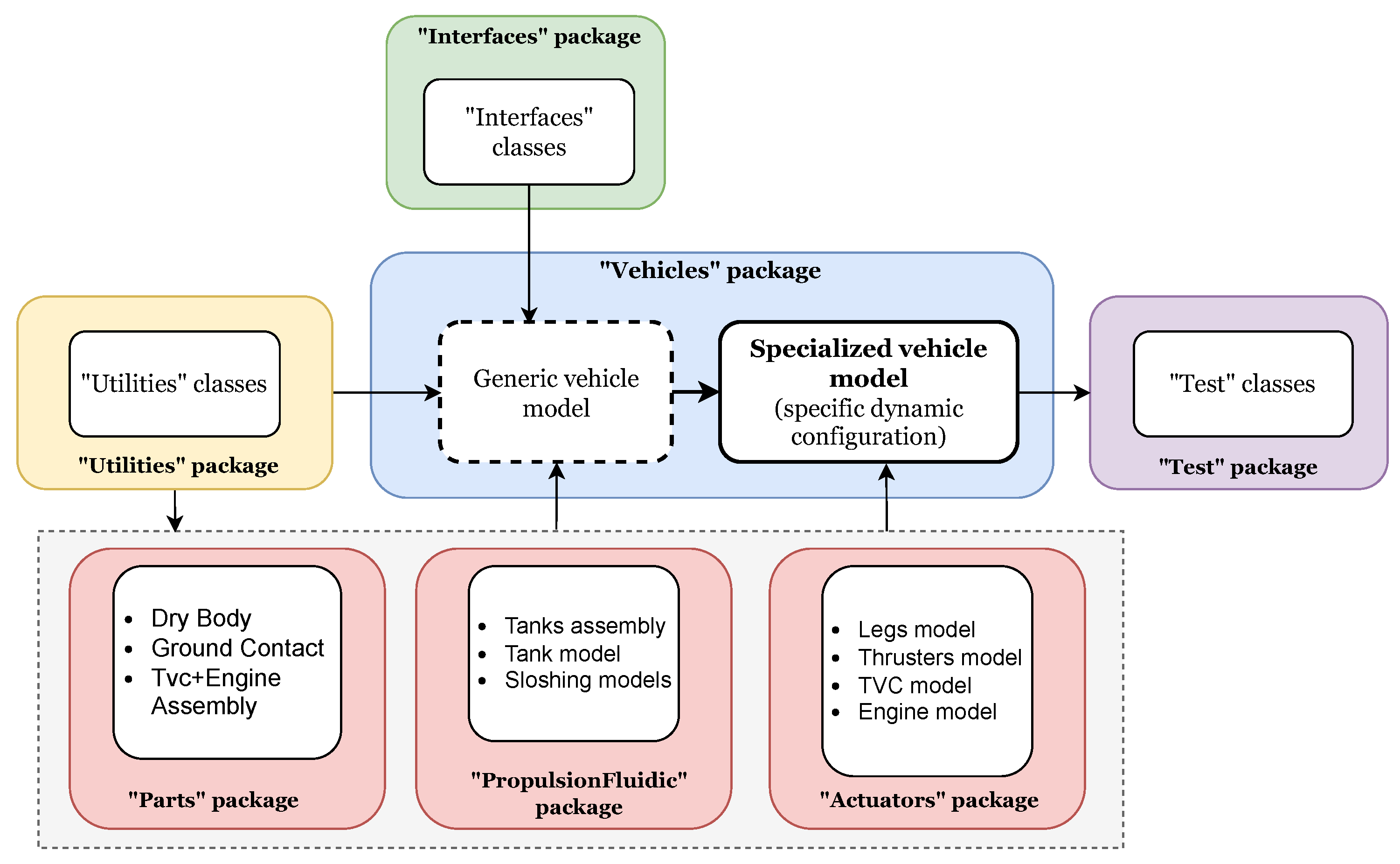
3.3. VLVLib Packages Description

The VLVLib is currently based on seven main packages (Figure 9) described below. Their functional dependencies are shown in Figure 10.
#1
The Vehicles package contains the base models of specific vehicles (e.g., Callisto) after extending the GenericVehicle partial model.
#2
Contains fundamental classes that concur in building the GenericVehicle class, but also specific dynamic effects (like flexibility) or actuator assemblies.
#3–4
Contain respectively the models for simulating the propulsion system and the actuator dynamics like the landing legs and TVC system.
#5
Includes utility classes of any type used across the library.
#6
Contains several unit tests of fundamental library models, including the vehicle ones.
#7
Contains the specialized vehicle models for the final export. For instance, the displayed Callisto_S_NL_NT model includes sloshing, but no TVC nor leg dynamics.

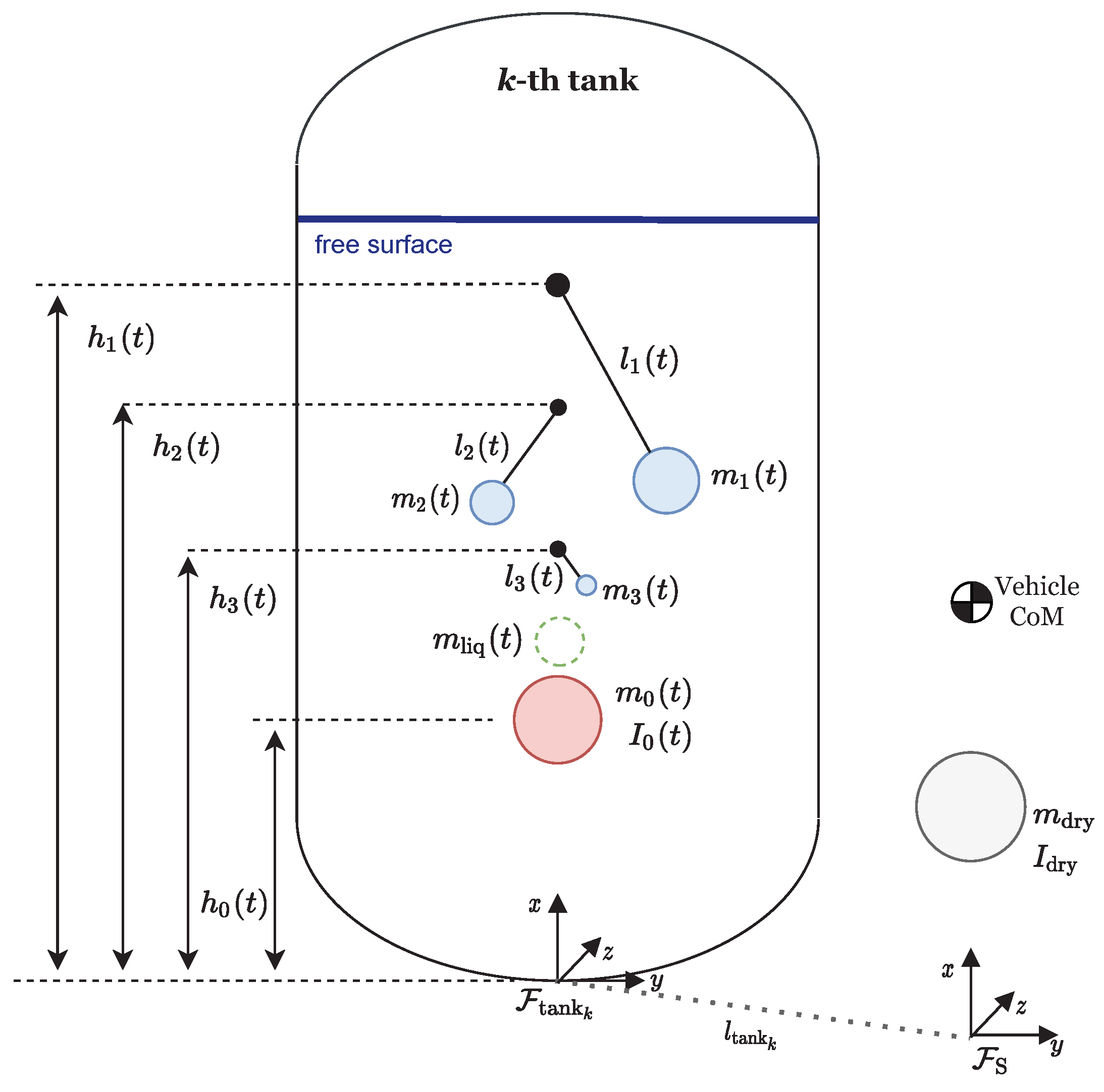
4. Propellant Slosh Dynamics Modeling

Lateral propellant slosh dynamics are a deeply studied phenomenon, and a well-known factor to consider in the GNC system design since the early days of large liquid-fuel rockets [29]. If the propellant contained in a tank has a free surface, parasitic interactions with its structure may arise as a result of the liquid movements. Normally, these adverse dynamics cannot be neglected, and should be appropriately tackled to avoid critical performance degradation or instability. From the GNC perspective, it has been demonstrated that a pendulum model can approximate the fluid dynamics of interest, provided that the sloshing natural frequencies are not excited [30]. When modeling sloshing via the pendulum analogy, the liquid in a tank is treated as a multibody system: one body represents the non-sloshing liquid mass (which is the largest fraction), whereas the remaining fraction is assigned to the sloshing mass of each pendulum. Three modes of oscillation are largely sufficient to characterize the main disturbances produced on the vehicle, since higher sloshing modes would have a small mass and a small impact on the whole dynamics.
The sloshing modeling within the VLVLib is extensively treated in [12]. The development requirements for the sloshing model are listed in Table 3. The first two ensure the model validity by preserving the liquid static MCI properties within a tank. The third ensures the model applicability to the multibody domain. The fourth states that the equivalent pendulum model characteristic parameters must vary according to the specific tank filling level for each mode [31]. The fifth guarantees model scalability, whereas the last requirement is essential to prevent a chaotic pendula motion when the vehicle experiences a quasi-zero non-gravitational acceleration (e.g., during no-thrust and no-aerodynamic drag phases). This is obtained by triggering a fictitious spring-damper system at each pendulum hinge point (see [12], Section 3.1.2).
Figure 11 depicts the explained model with the relevant parameters, alongside the key reference frames. The liquid mass is split into single pendulum masses m i and m 0 for the idle liquid. The non-sloshing mass m 0 , each pendulum mass m i and arm length l i , as well as the hinge heights h 0 and h i from the tank bottom, are defined for discrete tank filling levels, requiring interpolation during simulation. F S denotes the vehicle-structure-fixed frame, and F tank k is at the k-th tank bottom point. The MoI of the whole liquid is considered in I 0 . The dry vehicle is represented by a gray body with mass and inertia, respectively, labeled as m dry and I dry . Noticeably, the overall vehicle CoM position is affected not only by idle mass positioning, but also by the pendulum dynamics.
Note that the non-sloshing body model also embeds, alongside with the rigid-body equations, a term accounting for the change in the MoI ( I ˙ 0 ( t ) ) due to the propellant depletion. This term plays a big role in the vehicle dynamics, and cannot be neglected [21]. The liquid mass change m ˙ 0 ( t ) does not need to be included here if already accounted for in the engine thrust dynamics.
The liquid oscillation damping is also included and captured by a rotational damper at the pendulum hinge point. Its coefficient mainly depends on the vehicle longitudinal acceleration, the inherent liquid characteristics and the presence of extra damping devices (e.g., baffles). Its derivation is extensively explained in [31].

5. EMA-Based Thrust Vector Control Modeling

The TVC system needs two EMAs to deflect the engine thrust direction, and is essential to provide enough control authority to any launch vehicle. Its dynamics are often initially modeled as a first or second order dynamical system; however, it is a highly complex system composed of several elements.
An EMA operates thanks to the synergism of three parts: a Mechanical Power Transmission (MPT), to transform in the most efficient way a rotatory motion into a translational one; an Electric Motor (EM)—in this case a Permanent-Magnet Synchronous Motor (PMSM)—to produce the mentioned rotational motion; the Power Drive Electronics (PDE) part, to suitably power the EM using the available on-board electric source; and a control logic, to achieve the demanded EMA elongation resulting in the required engine thrust direction. They introduce several nonlinear changes in the overall actuator dynamics. A physical model of all these components is also beneficial to assess the performance of eventual model-based fault detection algorithms monitoring the TVC system [32]. The overall architecture is depicted in Figure 12. The modeling strategy and Modelica implementation details are extensively discussed in [20]. The key concepts are briefly recalled below.

5.1. Mechanical Power Transmission Modeling

The considered MPT is of direct-drive roller-screw type. Six models with incremental fidelity levels are proposed:
  • Level 1. It simply considers a perfect conversion of the motor torque and angular speed into a force and linear velocity, respectively.
  • Level 2. It adds a mechanical efficiency factor and an equivalent structural compliance (spring), capturing the whole transmission elasticity.
  • Level 3. It removes the efficiency factor and considers the mechanical degradation coming from the viscous friction. It includes the EMA screw mass as well.
  • Level 4. It adds Coulomb and Stribeck friction model contributions.
  • Level 5. It adds a friction component that depends on the loads induced by the engine dynamic condition.
  • Level 6. It adds the mechanical backlash and preload effects.
The MPT is normally the EMA component that influences the TVC closed-loop performance the most [20].

5.2. Electric Motor Modeling

The EM physical principles are the combination of effects acting in different physical domains: electrical, magnetic and mechanical. As such, the EM motor model choice affects the PDE interconnected model as well. The considered EM technology is an isotropic PMSM. Three models have been implemented:
  • Level 1. This is the simplest model, where the demanded torque is purely applied to the motor rotor rotational inertia.
  • Level 2. Here, the PMSM is physically modeled: the stator three-phase voltage and current equations can be written in a stationary reference frame. This transforms the three-phase machine into a two-phase machine, equipped with two windings fixed with the stator and orthogonal each other, expressed as d (‘direct’) and q (‘quadrature’), allowing for a more straightforward current closed loop design and analysis [33].
  • Level 3. It adds to EM Level 2 several dissipative effects: (i) friction losses; (ii) core losses (eddy current and hysteresis losses); (iii) permanent magnet losses; (iv) cogging torque. They are are included using the machine losses MSL’s package.

5.3. Power Drive Electronics Modeling

The PDE is meant to drive the EM model appropriately by producing the required phase voltages and currents with suitable hardware. Four PDE models are proposed. Note that, due to the different physical interfaces, two of them, PDE Level 1 and 2, would be only compatible with EM Level 1 model, whereas PDE models 3 and 4 would fit only EM Level 2 and 3 models (see [20], Sections 4.2 and 4.3 and Table 7):
  • Level 1. An input motor torque demand from the EMA control system is transferred directly to the EM as output. No dynamic is introduced.
  • Level 2. The motor torque outputted to the EM has second-order dynamics depending on the current loop natural frequency and its damping factor.
  • Level 3. This model implements the physical PDE dynamics to be connected with the motor. In this scenario, two closed loops are present to deal with the motor direct and quadrature currents. The motor torque demand is transformed into an appropriate quadrature current, responsible for the motor torque generation. The direct current is regulated to zero. These currents are transformed into a three-phase representations via an inverse Park transform. The voltage to produce such currents feeds the motor via an ideal generator.
  • Level 4. Adds to the Level 3 implementation the Pulse-Width Modulation (PWM) and inverter dynamics to command the required voltage to the EM. Introducing an inverter model is computationally heavy, so this fidelity level is not considered hereafter.

5.4. The EMA Control System

The EMA control system’s objective is to regulate the screw position to obtain the right TVC deflection, as per the reference input from the vehicle on-board computer. A classic scheme is constituted by a motor angular velocity and an outer stroke displacement control loops. The inner and outer controllers are proportional (P) and proportional–integral (PI) ones, respectively. The control gains can be tuned by simply imposing a damping ratio and natural frequency to the dynamical system resulting from the composition of the two loops. As said above, a third PI controller for the motor current is present. The current dynamics can be simplified for control synthesis as a first order transfer function with a pole dictated by the motor electrical resistance and inductance [33].

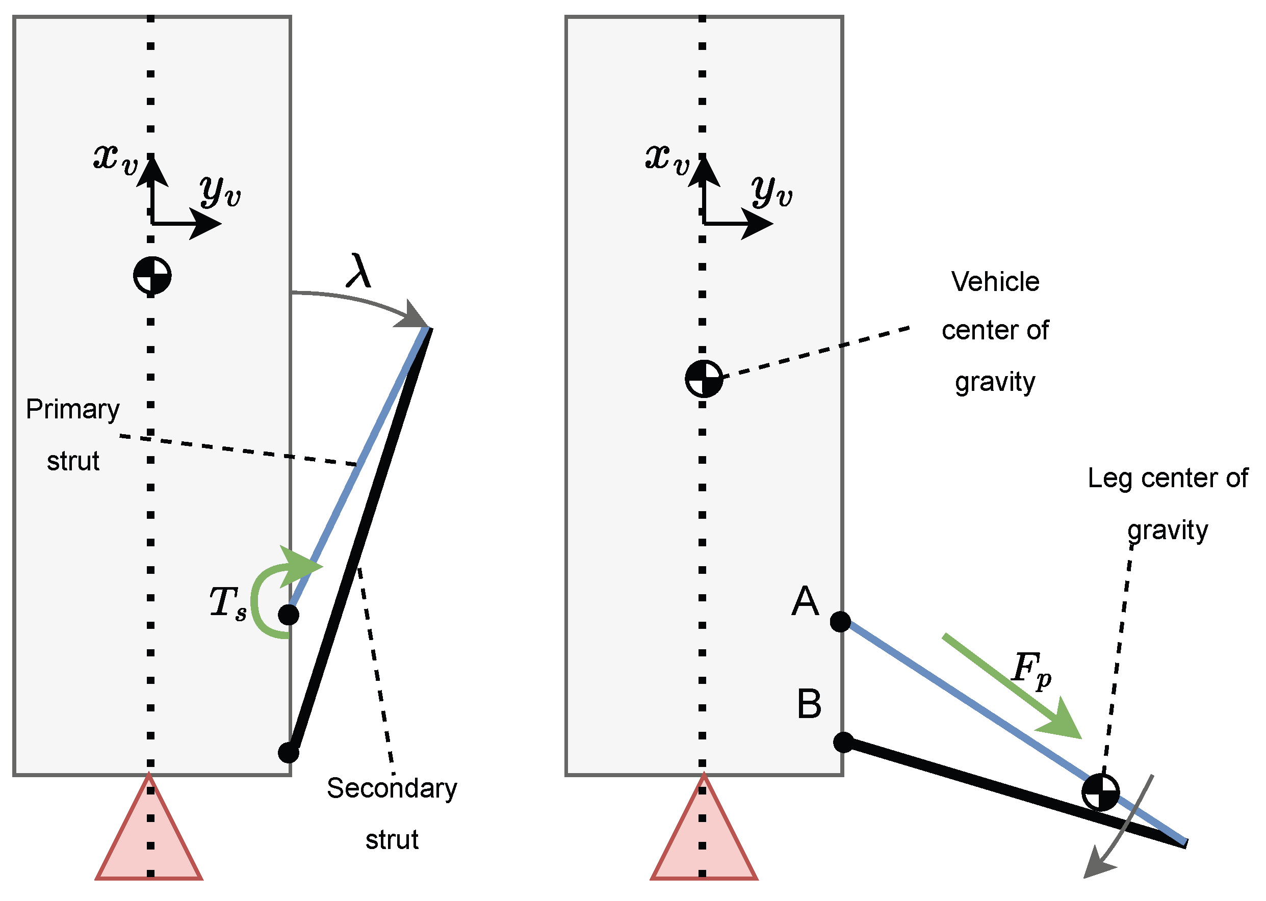
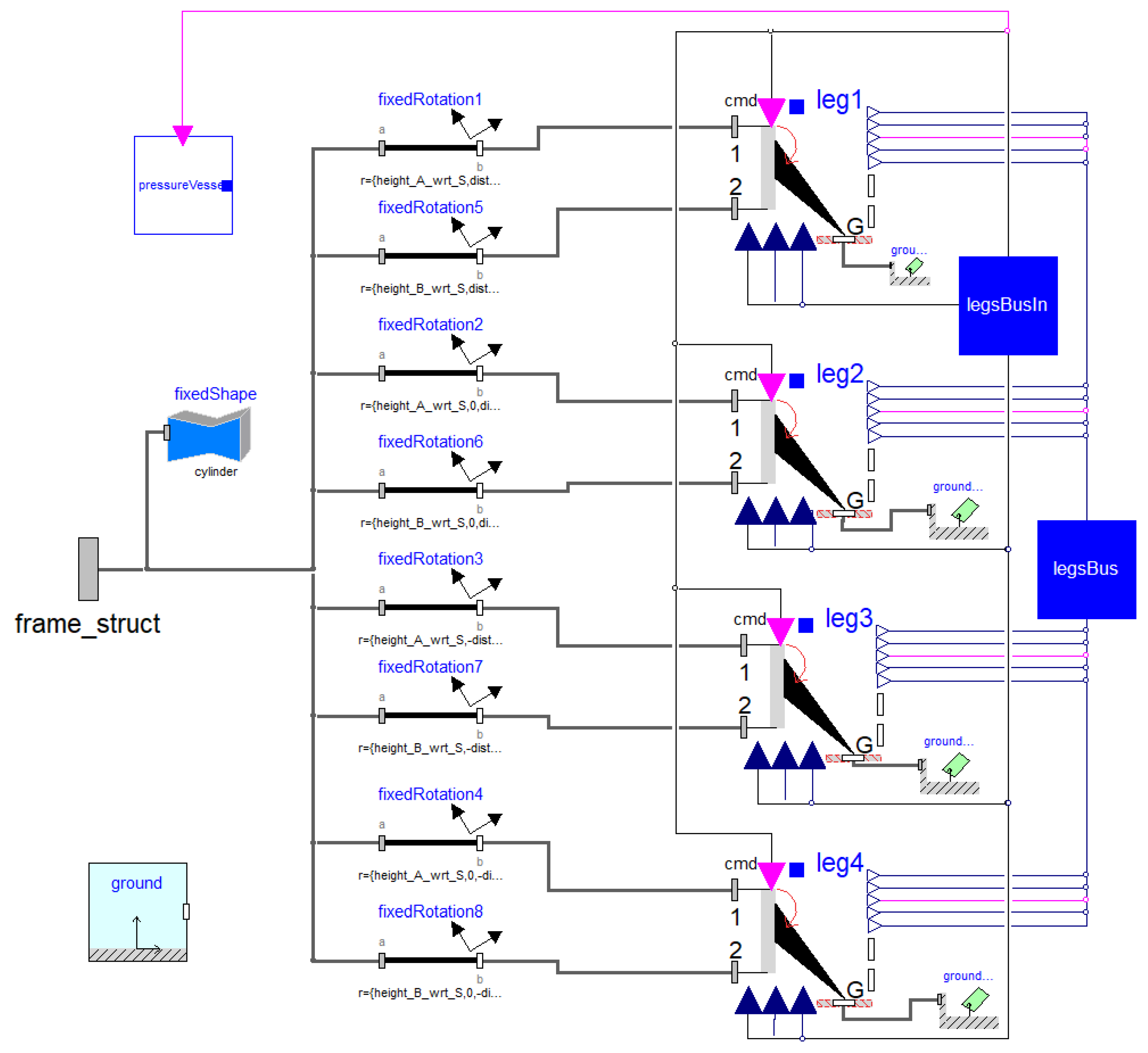
6. Landing Legs Deployment Model

Landing legs are fundamental for achieving reusability, because they enable a soft touchdown. A few moments before landing, the legs must be fully deployed; this is possible thanks to a mechanism able to release them from their folded configuration and push them outwards, such that gravity can start acting to further extract them and bring them towards their final latching position. However, gravity itself may not be sufficient to win the aerodynamic forces that strongly depend on the vehicle angle of attack, its velocity and the leg assembly orientation with respect to the wind vector. In fact, the more a leg is influenced by the aerodynamic drag, the longer it takes to open. Therefore, the deployment must be aided by additional forces to make sure that the legs can actually reach the fully unfolded configuration and latch in position. It is important to note that the vehicle longitudinal and lateral accelerations, the aerodynamics, and all the deployment mechanism forces and torques, are all coupled, strongly affecting, in turn, each individual leg deployment. This may cause an asymmetry in their unfolding which, consequently, generates unbalanced internal forces and torques on the vehicle core. This effect must be accounted for in detail at the GNC design phase to make sure that there is sufficient margin for the control system to compensate for it before touchdown.
The discussed four-leg model is based on CALLISTO, and is fully explained and analyzed in [19]. Figure 13 shows the main model quantities. The variable λ defines each leg opening angle. The primary strut can be seen as a telescopic rod enabling the legs unfolding and operating thanks to a helium-based pneumatic system that generates an opening force F p (net of the occurring friction). The secondary strut, instead, is in charge of withstanding the heat stress and holding the vehicle in position after touchdown. Note that the pressure in each leg primary strut depends on the available pressure throughout the pipes and the source pressure vessel; therefore, the deployment rate of each leg indirectly affects the others as well. When a leg is completely deployed, a latching mechanism locks it in position. Lastly, a release spring produces a torque T s to initiate the leg unfolding.
The Modelica implementation details are discussed in Appendix A.

7. Ground Contact Modeling

The problem of modeling body impacts has been already addressed in [34,35]. Having an accurate representation of the behavior of the vehicle when it touches the ground may provide useful insights into the vehicle stability and the terminal landing conditions to be fulfilled to avoid vehicle tipping and its subsequent damage.
Here, the penalty-based approach described in [34] is used, where a high elastic and damping force is applied to the impacting body on the principles of a spring-damper mechanism. Despite this implies a high computational cost, the dynamic is short and triggered only at the end of the mission.
The implementation details are in Appendix B.

8. Simulation Results

In this section, simulation results are shown for the four main considered dynamics with representative examples carried out onto CALLISTO rocket end-to-end mission, designed with an ascent, boostback, aerodynamic and landing phases. The goal is to understand how the four described effects manifest and impact the vehicle dynamics. The simulations are run with the current Guidance and Control system, and assume perfect Navigation algorithms [36]. All simulations have unperturbed parameters and no wind disturbance. The simulations are run with one dynamic effect at a time; for instance, when analyzing the sloshing, no physical TVC or leg deployment models are included.

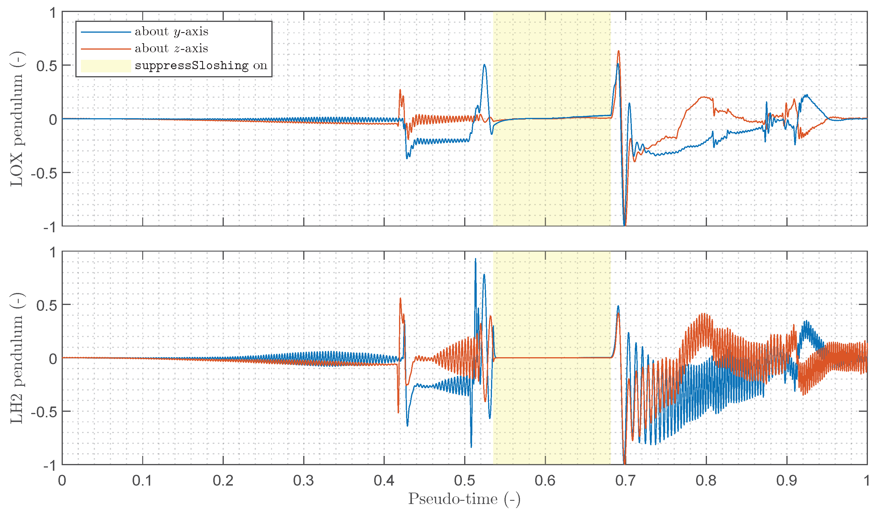
8.1. Sloshing Dynamics

CALLISTO has two tanks, one for the oxidizer (liquid oxygen—LOX) and one for the fuel (liquid hydrogen— LH 2 ). They are full at take off; for both, only one sloshing mode is accounted for at this stage.
In Figure 14, LOX and LH 2 tank pendulum angles with respect to vehicle y- and z-axes ( F S frame in Figure 11) are shown. Each angle profile has been normalized with respect to the absolute value of its maximum over the entire flight. The validity boundaries for the sloshing model must not exceed the quasi-linear pendulum dynamic region (i.e., angles must be between ± 20 deg). Correlation with the real angle magnitudes cannot be explicitly given; however, the validity boundaries for pendulum models are not exceeded across the entire flight. At boostback, the vehicle experiences a quasi-zero non-gravitational acceleration on its longitudinal axis; in this phase, the liquid undergoes a chaotic motion and spreads in the tank. From a simulation viewpoint, this implies that the equivalent sloshing model is not valid anymore, and the pendulum motion must be inhibited. In fact, Figure 14 evidences how, in the highlighted area where suppressSloshing=true, the pendulum restores its neutral position and stops oscillating.
Figure 15 shows the impact of sloshing during the ascent phase: two simulations were run, one with simple rigid-body dynamics and one with the rocket multibody dynamics featuring the described sloshing model. The angular rates (expressed with respect to the body frame, i.e., a translation of F S into the vehicle CoM) of the latter simulation are then subtracted to those of the former one in order to highlight the effect of sloshing. We focus on the rates about y- and z - axes, since rolling motion is only marginally affected: after normalization with respect to the maximal values of the rigid-body simulation, the angular rates have grown in magnitude by up to 25%. This also reflects into large position errors, and shows how sloshing, if not accounted for properly at GNC level, can potentially determine the failure of a mission.

8.2. TVC System

In order to understand the impact of the higher-fidelity TVC dynamics, two types of simulations are compared: one with a rigid-body vehicle model, featuring a linear TVC actuator model implemented as a transfer function (details can be found in [20]). In this case, the TWD effect is absent, as well as the advanced PDE, EM and MPT dynamics. A second simulation is performed, instead, with the Modelica multibody vehicle model, including the TVC dynamics determined by the two EMAs with PDE Level 3, EM Level 3 and MPT Level 6 models. Furthermore, the inertial properties of the movable engine part is simulated with another rigid body having the right MCI properties, thus the TWD effect is captured too. Note that, with such models, the TVC angle saturation can be implemented only by means of hard physical stops, hence as rotational spring-damper systems simulating a collision with the engine bay. As such, the inclusion of elasticity within advanced MPT models helps with assessing whether the TVC control system keeps the movable load sufficiently far from potential structural crashes with the engine bay.
In Figure 16, the TVC, rotations about the y- and z-axes are shown during the ascent phase. Each angle has been normalized with respect to the time-wise maximum of its absolute value in the rigid-body simulation case. The chattering effect is due to the mechanical backlash and pre-load spring: despite the commanded angles are relatively low during ascent, it is the phase when the backlash effect highlights the most by significantly increasing the TVC angle deflection tracking error. Consequently, the vehicle angular rates (Figure 17) are also influenced, showing a relevant impact on the vehicle performance. The plots are normalized as for sloshing. It is anyhow worth mentioning that the TVC dynamics include a closed-loop system, therefore the added dynamics of the higher-fidelity TVC models are mostly highlighted at high frequency, or in specific phases like the toss-back maneuver when the higher loads on the EMAs may increase the MPT friction.

8.3. Legs Deployment and Touchdown Dynamics

When the leg deployment command is triggered, the vehicle dynamic state deeply affects the opening of each leg. During the landing phase, the vehicle may have a non-null angle of attack and side-slip angle, and the lateral accelerations may not be small. In Figure 18, the leg opening angle profiles are shown; the asymmetry in the deployment is the responsible for the generation of forces and torques acting on the vehicle core body. At the deployment start, the driving opening force is the release spring mechanism, while afterwards the pneumatic system is the main contributor. The latter force tends to diminish after a certain λ angle and makes the deployment rate steady. In Figure 19, the vehicle angular rates are shown as compared to a simulation where the vehicle model is a rigid body without legs. Normalization is performed similarly to the previous plots. Because the legs constitute a relevant fraction of the whole vehicle mass at landing, the extra contribution coming from the four leg forces and torques can severely increase the magnitude of the vehicle angular rates, ultimately highlighting the relevance of capturing the legs deployment with appropriate multibody simulation models.
To analyze the touchdown dynamics, an ad hoc simulation was performed. The simulation is initialized with the rocket having an attitude of 1deg about the y-axis and 5deg about the z-axis (with respect to an inertial frame), while the ground impact velocity is close to the limit imposed by the related requirement. The initial angular rates are close to zero. This scenario is meant to cause an asynchronous touchdown between each leg. Figure 20 depicts the angular rates after the impact, while Figure 21 captures the distance of each leg from the ground. Due to the imposed initial states, at touchdown, the vehicle is induced to spin about its x-axis until two of the legs have persistent contact with the ground. Then, the vehicle starts wobbling intermittently until the motion damps out. Although the vehicle does not undergo any tipping, the leg rebound gets up to 0.4 m. Consequently, it becomes clear how the final vehicle stability on the landing pad depends on the touchdown attitude, but also on the ground-leg stiffness and damping factors. This type of simulation aids identifying potential flaws in the landing GNC algorithms or requirement definitions.

9. Conclusions

This paper extensively explored many aspects of the advanced physical modeling and simulation of reusable rockets for GNC V&V. The dynamics required for RLV modeling were detailed, and a suitable methodology was proposed to develop a scalable, responsive, and adaptable framework for modeling and simulating these dynamics. This facilitates a closer alignment with the specific demands of various development phases.
We showed the potential of the VLVLib, a Modelica library that implements several key dynamics in order to obtain higher-fidelity multibody vehicle models with respect to more standard approaches relying on rigid-body assumptions. The modeling and implementation rationale was explained and proved successful for achieving flexibility when creating models with different fidelity levels, as well as managing the large amount of models and parameters. In this sense, Modelica language features were explained and suitably exploited. Four main dynamics affecting the vehicle’s overall behavior were investigated, and the modeling strategy for each was explained. These dynamics include propellant sloshing, the TVC system dynamics, the deployment of landing legs, and landing touchdown dynamics. They were simulated to highlight their detrimental effect on the vehicle performance with respect to plain rigid-body models, demonstrating the framework potentiality to discover GNC system flaws during Monte-Carlo campaigns, but also badly posed requirements. The CALLISTO rocket was used as benchmark. Also, this paper demonstrates the framework applicability to common RLV development workflows, as the proposed physical Modelica models were successfully integrated into a pre-established Simulink®-based framework. This avoided unnecessary replication of well-tested functions and showed that such existing simulation environment can be successfully extended.
In conclusion, the methodology presented in this paper proved its potential in integrating the GNC modeling, simulation and V&V work logic within any stage of a reusable launch vehicle development process.

Author Contributions

Conceptualization, investigation and methodology: S.F.; Software: S.F., J.A.M.H., M.S. (Marco Sagliano), A.S., A.H. and M.S. (Markus Schlotterer); Validation: S.F., J.A.M.H. and M.S. (Marco Sagliano); Writing—original draft preparation: S.F. and M.S. (Marco Sagliano); Writing—review and editing: S.F. and M.S. (Marco Sagliano); Supervision: M.S. (Markus Schlotterer) and S.W. All authors have read and agreed to the published version of the manuscript.

Funding

This research received no external funding.

Data Availability Statement

The data presented in this study are available in the article.

Acknowledgments

The authors thank Stephan Theil and David Seelbinder (German Aerospace Center–DLR) for supporting and enabling this work; Pedro Simplicio (European Space Agency–ESA) for providing invaluable guidance to the TVC modeling part; Riccardo Minnozzi (TU Delft) for his fundamental help in testing the VLVLib and integrating the whole software.

Conflicts of Interest

The authors declare no conflicts of interest.

Abbreviations

The following abbreviations are used in this manuscript:
CALLISTOCooperative Action Leading to Launcher Innovation in Stage Toss back Operations
CNESCentre National d’Études Spatiales
CoMCenter of Mass
DAEDifferential-Algebraic system of Equations
DLRDeutsches Zentrum für Luft- und Raumfahrt (English: German Aerospace Center)
DoFDegrees-of-Freedom
EMElectric Motor
EMAElectro-Mechanical Actuator
FMIFunctional Mock-up Interface
FMUFunctional Mock-up Unit
GNCGuidance, Navigation and Control
IDEIntegrated Development Environment
JAXAJapan Aerospace Exploration Agency
MCIMass-Centering-Inertia
MoIMoment of Inertia
MPTMechanical Power Transmission
MSLModelica Standard Library
PDEPower Drive Electronics
PMSMPermanent-Magnet Synchronous Motor
PWMPulse-Width Modulation
RCSReaction Control System
RLVReusable Launch Vehicle
TVCThrust Vector Control
TWDTail-Wags-Dog
V&VValidation and Verification
VLVLibVertical Landing Vehicles Library
VTVLVertical Take-off, Vertical Landing

Appendix A. Landing Legs Deployment Library Implementation

The difficulty for the implementation of a leg unfolding simulation model is that its mechanical structure is a closed kinematic chain. Normally, with an open chain configuration the compiler is able to solve for the states of the next chain elements based on the current one. In closed chains, for each body there exists more than one path connecting to a uniquely defined set of states. Closed chains can be structurally non-singular or singular. This means that they can generate statically indeterminate systems (more equations than unknowns), as often happens in planar closed chains. The software symbolic manipulation applicable to a generic DAE system can not distinguish between consistent statically indeterminate systems (for which would be enough to ignore some equations) and inconsistent systems (thus defined by contradictory equations). The structural singularity of the DAE system is detected and the compilation fails. It is therefore necessary to eliminate the redundant equations before applying the symbolic manipulation beforehand. As the nonlinear algebraic constraints arising from most mechanical loops may not be always automatically solved by the Modelica translator, the MSL includes a set of components where a predefined set of joints are already considered together, and the resulting equations of motion pre-solved and implemented. As such, when these joint assemblies take part into a closed chain, the solver becomes able to solve for it.
The component jointRRP implemented in the class LegCallisto (Figure A1) is one of those, and was instantiated for that reason. The same figure also shows how the primary and secondary struts are implemented. The release mechanism acts as a torque at point A, generated by a torsional spring active only when the deployment command has been triggered and λ angle is small (i.e., less that 1deg). The Boolean deployment command input is latched internally by a flip-flop (top-left of the figure), such that the depending conditional expressions can be consistently used to manage the force and torque acting on the leg. The leg separation is obtained via separateLeg component which, when the trigger signal is ‘true’, allows a rotational degree of freedom at point B to let the leg move. Note that a connector frame_ground is present. This allows the leg model to simulate the ground contact at the tip of the primary strut. LegsAssembly (Figure A2) model instantiates the four legs and is included in the main Callisto model.
Figure A1. LegCallisto model diagram view. Some connections are specified only in the code without visual attributes (no connecting lines).
Aerospace 11 00337 g0a1
Figure A2. LegsAssembly model diagram view.
Aerospace 11 00337 g0a2

Appendix B. Ground Contact Library Implementation

The VLVLib approach to simulate ground impact requires two models: Ground and GroundForce. The first contains all the properties for defining where the actual “ground” is located. This is fundamentally a fixed translation with respect to an Earth-Centered Earth-Fixed (ECEF) frame. In this way, the “flat” ground resembling the actual landing pad can be moved throughout the simulation with the Earth rotation, thus avoiding to start the contact ahead of time. The same class also contains the definition of the “vertical” axis (“off-ground”) and the “horizontal” axes (“on-ground”) of the local ground frame. A Ground class defines all the properties of the ground (e.g., position, orientation, dampting properties, etc.), which should be available throughout the entire model hierarchy. For this reason, it must be instantiated with the inner attribute, making its states and parameters available to all models down the hierarchy whenever another Ground component is declared with the outer attribute.
This is what happens in the GroundForce model (Figure A3), responsible for the generation of the ground reaction forces and torques: it connects the physical mechanical connector that must “expose” to the ground contact to the Ground mechanical connector itself, but it allows for all degrees of freedom in between (three rotational and three translational). With this construction, we can exert specific forces and torques only when contact is occurring and not otherwise. Along the “vertical” axis, an ElastoGap model from the MSL is used to model the vertical rebound: when the ground is reached, a spring-damper mechanism triggers to avoid the penetration of the impacting body into the ground. The contact presence is governed by the ElastoGap.contact Boolean variable. Also, when it is ‘true’, some breaking forces act on the remaining two translational degrees of freedom to avoid that the impacting body unnaturally “slips” sideways onto the ground surface.
Figure A3. Exemplification of the ElastoGap.contact usage within GroundForce model.
Aerospace 11 00337 g0a3

References

  1. Blackmore, L. Autonomous Precision Landing of Space Rockets. Natl. Acad. Eng. Bridge Front. Eng. 2016, 4, 15–20. [Google Scholar]
  2. Hoffman, L.; Baker, M.; Glynn, S.; Darley, M.; Beck, P. Reusable Electron: Analysis of Progress Toward the World’s First Reusable Commercial Small Rocket. In Proceedings of the Small Satellite Conference, Logan, UT, USA, 6–11 August 2022. [Google Scholar]
  3. Dumont, E.; Illig, M.; Ishimoto, S.; Chavagnac, C.; Saito, Y.; Krummen, S.; Eichel, S.; Martens, H.; Giagkozoglou, S.; Häseker, J.S.; et al. CALLISTO: A Prototype Paving the Way for Reusable Launch Vehicles in Europe and Japan. In Proceedings of the 73rd International Astronautical Congress (IAC), Paris, France, 18–22 September 2022. [Google Scholar]
  4. Dumont, E.; Ecker, T.; Chavagnac, C.; Witte, L.; Windelberg, J.; Klevanski, J.; Giagkozoglou, S. CALLISTO—Reusable VTVL Launcher First Stage Demonstrator. In Proceedings of the Space Propulsion Conference, Seville, Spain, 14–18 May 2018. [Google Scholar]
  5. Bertorello, C.; Gogdetb, O.; Breteauc, J.; Tincelind, Y.; Cliquet-Moreno, E.; Coletti, E.; Bensalem, S. Themis Demonstration Programme. In Proceedings of the 73rd International Astronautical Congress (IAC), Paris, France, 18–22 September 2022. [Google Scholar]
  6. Gallego, P. MIURA 5: The European and Reusable Microlauncher for CubeSats and Small Satellites. In Proceedings of the Small Satellite Conference, Logan, UT, USA, 1–6 August 2020. [Google Scholar]
  7. Patureau de Mirand, A.; Bahu, J.M.; Gogdet, O. Ariane Next, a Vision for the next Generation of Ariane Launchers. Acta Astronaut. 2020, 170, 735–749. [Google Scholar] [CrossRef]
  8. Strauch, H.; Luig, K.; Bennani, S. Model Based Design Environment for Launcher Upper Stage GNC Development. In Proceedings of the Workshop on Simulation on for European Space Programmes (SESP), ESA/ESTEC, Noordwijk, The Netherlands, 24–26 March 2015. [Google Scholar]
  9. Gäßler, B.; Briese, L.E.; Acquatella B., P.; Simplício, P.; Bennani, S.; Casasco, M. Design and Development of R2M2—A Multi-Physics Modeling Tool for Reusable Launch Vehicles. In Proceedings of the 9th International Conference on Astrodynamics Tools and Techniques (ICATT), Sopot, Poland, 12–16 June 2023. [Google Scholar]
  10. Farì, S.; Grande, D. Vector Field-based Guidance Development for Launch Vehicle Re-entry via Actuated Parafoil. In Proceedings of the 72nd International Astronautical Congress (IAC), Dubai, United Arab Emirates, 25–29 October 2021; Available online: https://elib.dlr.de/145123 (accessed on 20 April 2024).
  11. Gutierrez, J.L.R.; Farì, S.; Winter, M. Control System Design for the ALINA Lunar Lander. In Proceedings of the 72nd International Astronautical Congress (IAC), Dubai, United Arab Emirates, 25–29 October 2021; Available online: https://elib.dlr.de/145129 (accessed on 20 April 2024).
  12. Farì, S.; Seelbinder, D.; Theil, S. Advanced GNC-oriented Modeling and Simulation of Vertical Landing Vehicles with Fuel Slosh Dynamics. Acta Astronaut. 2022, 204, 294–306. [Google Scholar] [CrossRef]
  13. Looye, G. The New DLR Flight Dynamics Library. In Proceedings of the 6th Modelica Conference, Bielefeld, Germany, 3–4 March 2008. [Google Scholar]
  14. Pulecchi, T.; Casella, F.; Lovera, M. A Modelica Library for Space Flight Dynamics. In Proceedings of the 5th International Modelica Conference, Vienna, Austria, 4–5 September 2006. [Google Scholar]
  15. Briese, L.E.; Schnepper, K.; Acquatella B., P. Advanced Modeling and Trajectory Optimization Framework for Reusable Launch Vehicles. In Proceedings of the 2018 IEEE Aerospace Conference, Big Sky, MT, USA, 3–10 March 2018. [Google Scholar] [CrossRef]
  16. Acquatella, P.; Reiner, M.J. Modelica Stage Separation Dynamics Modeling for End-to-End Launch Vehicle Trajectory Simulations. In Proceedings of the 10th International Modelica Conference, Lund, Sweden, 10–12 March 2014. [Google Scholar]
  17. Farì, S. The Vertical Landing Vehicles Library (VLVLib): A Modelica-based Approach to High-Fidelity Simulation and Verification of GNC Systems for Reusable Rockets. In Proceedings of the 73rd International Astronautical Congress (IAC), Paris, France, 18–22 September 2022; Available online: https://elib.dlr.de/188514 (accessed on 20 April 2024).
  18. Martin, C.; Urquia, A.; Sanchez, J.; Dormido, S. Interactive Simulation of Object-Oriented Hybrid Models, by Combined Use of Ejs, Matlab/Simulink and Modelica/Dymola. In Proceedings of the 18th European Simulation Multiconference, Magdeburg, Germany, 13–16 June 2004. [Google Scholar]
  19. Schneider, A.; Desmariaux, J.; Klevanski, J.; Schröder, S.; Witte, L. Deployment Dynamics Analysis of CALLISTO’s Approach and Landing System. CEAS Space J. 2023, 15, 343–356. [Google Scholar] [CrossRef]
  20. Farì, S.; Seelbinder, D.; Theil, S.; Simplicio, P.; Bennani, S. Physical Modeling and Simulation of Electro-Mechanical Actuator-Based TVC Systems for Reusable Launch Vehicles. Acta Astronaut. 2024, 214, 790–808. [Google Scholar] [CrossRef]
  21. Gäßler, B.; Briese, L.E.; Acquatella B., P.; Simplício, P.; Bennani, S.; Casasco, M. Variable-Mass Dynamics Implementation in Multi-Physics Environment for Reusable Launcher Simulations. In Proceedings of the 9th European Conference for Aeronautics and Space Sciences (EUCASS-3AF), Lille, France, 27 June–1 July 2022. [Google Scholar] [CrossRef]
  22. Modelica Association. Modelica Standard Library. Available online: https://github.com/modelica/ModelicaStandardLibrary (accessed on 20 April 2024).
  23. Otter, M.; Elmqvist, H.; Mattsson, S.E. The New Modelica MultiBody Library. In Proceedings of the 3rd International Modelica Conference, Linköping, Sweden, 3–4 November 2003. [Google Scholar]
  24. The MathWorks, Inc. Implement Variations in Separate Hierarchy Using Variant Subsystems. Available online: https://www.mathworks.com/help/simulink/ug/variant-subsystems.html (accessed on 20 April 2024).
  25. Modelica Association. Functional Mock-up Interface. Available online: https://fmi-standard.org (accessed on 20 April 2024).
  26. Brück, D.; Elmqvist, H.; Mattsson, S.E.; Olsson, H. Dymola for Multi-Engineering Modeling and Simulation. In Proceedings of the 2nd International Modelica Conference, Starnberg, Germany, 18–19 March 2002. [Google Scholar]
  27. Fritzson, P. Principles of Object-Oriented Modeling and Simulation with Modelica 3.3: A Cyber-Physical Approach; John Wiley & Sons: Hoboken, NJ, USA, 2014. [Google Scholar]
  28. Modelica Association. Modelica Specification. Available online: https://specification.modelica.org (accessed on 20 April 2024).
  29. Bayle, O.; L’Hullier, V.; Ganet, M.; Delpy, P.; Francart, J.L.; Paris, D. Influence of the ATV Propellant Sloshing on the GNC Performance. In Proceedings of the AIAA Guidance, Navigation, and Control Conference and Exhibit, Monterey, CA, USA, 5–8 August 2002. [Google Scholar] [CrossRef]
  30. Abramson, H.N. Dynamic Behavior of Liquids in Moving Containers with Applications to Space Vehicle Technology; Special Publication (SP) 19670006555; NASA: Washington, DC, USA, 1966.
  31. Dodge, F.T.; Antonio, S. The New “Dynamic Behavior of Liquids in Moving Containers”; Southwest Research Inst.: San Antonio, TX, USA, 2000. [Google Scholar]
  32. Farì, S.; Seelbinder, D.; Theil, S.; Simplicio, P.; Bennani, S. Sensor Fault Detection and Isolation for Electro-Mechanical Actuators in a Reusable Launch Vehicle TVC System. In Proceedings of the 10th European Conference For Aeronautics And Space Sciences (EUCASS), Lausanne, Switzerland, 9–15 July 2023. [Google Scholar] [CrossRef]
  33. Krishnan, R. Permanent Magnet Synchronous and Brushless DC Motor Drives, 1st ed.; CRC Press: Boca Raton, FL, USA, 2017. [Google Scholar]
  34. Hofmann, A.; Mikelsons, L.; Gubsch, I.; Schubert, C. Simulating Collisions within the Modelica MultiBody Library. In Proceedings of the 10th International Modelica Conference, Lund, Sweden, 10–12 March 2014; pp. 949–957. [Google Scholar] [CrossRef]
  35. Oestersötebier, F.; Wang, P.; Trächtler, A. A Modelica Contact Library for Idealized Simulation of Independently Defined Contact Surfaces. In Proceedings of the 10th International Modelica Conference, Lund, Sweden, 10–12 March 2014; pp. 929–937. [Google Scholar] [CrossRef]
  36. Sagliano, M.; Tsukamoto, T.; Maces Hernandez, J.A.; Seelbinder, D.; Ishimoto, S.; Dumont, E. Guidance and Control Strategy for the CALLISTO Flight Experiment. In Proceedings of the 8th European Conference for Aeronautics and Space Sciences (EUCASS), Madrid, Spain, 1–4 July 2019. [Google Scholar] [CrossRef]
Figure 1. Highlights of the role of incremental-fidelity physical simulation models within the GNC design and V&V iterative process.
Aerospace 11 00337 g001
Figure 2. Illustration of the relevant dynamics in the CALLISTO reusable rocket’s modeling and simulation framework for GNC Validation and Verification.
Aerospace 11 00337 g002
Figure 3. Depiction of the framework architecture built in Simulink® with embedded vehicle multibody model as FMUs. Some lines are dashed for visual clarity.
Aerospace 11 00337 g003
Figure 4. Architecture-driven example scheme. Blue connectors are casual, whilst black ones have no direction, hence acausal. All components can be replaced with other variants provided the old and new interfaces match.
Aerospace 11 00337 g004
Figure 5. Example of the architecture-driven approach and component redeclaration.
Aerospace 11 00337 g005
Figure 6. Record classes used for data component handling within models (from [20]).
Aerospace 11 00337 g006
Figure 7. Callisto model Modelica code.
Aerospace 11 00337 g007
Figure 8. Callisto model diagram view. Some connections are specified only in the code without visual attributes (no connecting lines).
Aerospace 11 00337 g008
Figure 9. Listing of the current VLVLib packages and their first sub-level content.
Aerospace 11 00337 g009
Figure 10. VLVLib packages functional dependencies.
Aerospace 11 00337 g010
Figure 11. Planar representation of the employed pendulum equivalent model (from [12]).
Aerospace 11 00337 g011
Figure 12. Simplified planar TVC architecture using an electro-mechanical actuator (from [20]).
Aerospace 11 00337 g012
Figure 13. Simplified view of the legs model. The primary and secondary strut hinge points are marked as ‘A’ and ‘B’, respectively.
Aerospace 11 00337 g013
Figure 14. CALLISTO normalized LOX and LH 2 pendulum angles in an end-to-end simulation.
Aerospace 11 00337 g014
Figure 15. Sloshing impact on the vehicle angular rates: difference between a multibody vehicle model with sloshing and a simple rigid-body model without sloshing (ascent phase only).
Aerospace 11 00337 g015
Figure 16. TVC angular displacements: simulation with a multibody vehicle model with multi-physics TVC dynamics vs. a rigid-body vehicle model with linear TVC dynamics.
Aerospace 11 00337 g016
Figure 17. TVC modeling impact on angular rates: difference between multibody vehicle model with multi-physics TVC dynamics and rigid-body with linear TVC dynamics (ascent only).
Aerospace 11 00337 g017
Figure 18. Normalized leg opening angles during deployment.
Aerospace 11 00337 g018
Figure 19. Legs modeling impact on the vehicle angular rates: difference between a physical multibody model including the leg dynamics and a simple rigid-body model.
Aerospace 11 00337 g019
Figure 20. Angular rates of the body frame with respect to inertial frame (expressed in body frame) at touchdown.
Aerospace 11 00337 g020
Figure 21. Leg tip distances from ground at touchdown.
Aerospace 11 00337 g021
Table 1. Brief review of the major modeled dynamics for CALLISTO rocket (alphabetical order).
Dynamic EffectDescription
AerodynamicsThe aerodynamics are included by computing the generated forces and torques from ad hoc interpolation tables with respect to quantities like angle of attack, side-slip angle, Mach number and engine thrust. The tables normally come from computational fluid dynamics analyses, eventually adjusted by experiments. They also include dependencies with respect to each aerodynamic fin deflections and each landing leg opening angle.
Aerodynamic finsEach fin’s aerodynamics are mainly included in the aforementioned aerodynamic look-up tables. Their deployment dynamics, however, influence the Mass-Centering-Inertia (MCI) vehicle properties by shifting the overall Center of Mass (CoM) and changing the overall vehicle Moment of Inertia (MoI). The deployment generates reaction forces and torques to the vehicle, but due to their relatively low mass, it could be neglected.
Dry vehicle dynamicsThe dry vehicle (no propellant considered) inertial properties are captured as a specific body. Naturally, it has to be always included in any RLV model.
Engine thrust dynamicsThe engine dynamics depend on environment properties during flight, like the air density. The thrust characteristics are obtained via interpolation tables after experimental testing and injected in the vehicle dynamics as an external force at the right application point.
Ground contact *The landing legs interact with the ground at the moment of touchdown, therefore the vehicle tipping depends on if and how ground contact is modeled. The impact reaction forces and torques to each leg depend on the ground stiffness and damping properties, as well as those of the legs themselves.
Landing legs *The deployment of landing legs has a similar impact on the whole vehicle MCI as for the fins. Furthermore, their mass is not negligible, and the deployment dynamics depend on several factors, like the pneumatic system, the release springs, or the aerodynamic resistance. Hence, the resulting impact on the vehicle dynamics is relevant. Each leg is composed of several bodies connected in a closed kinematic loop; this makes each leg model, per se, multibody [19].
Propellant depletionAs the propellant gets depleted, the remaining mass within the tank decreases, thus altering the overall vehicle MCI. This is due to both the fuel and oxidizer, but also to the RCS propellant.
Propellant slosh dynamics *The propellant is subject to lateral sloshing motion, captured via a spherical pendulum mechanical equivalent. Each pendulum represents a fraction of the liquid mass in a tank, and must approximate the sloshing behavior at each tank filling level, for which specific parameters are available. The vehicle overall CoM and MoI properties are influenced by the pendula motion.
Reaction Control System (RCS)The thrust direction of the RCS is normally fixed, whereas the thrust level depends on the air density. A simple model of the thrust profile of each thruster can be used and applied to the vehicle as external force at the right application point.
Structural flexibilityThe vehicle experiences bending due to all the forces and torques acting on it, mainly aerodynamics, engine thrust, sloshing and control fins. The rocket flexibility heavily depends on the remaining propellant mass. Bending modeling can be tackled by adopting a linear combination of independent bending modes to describe the bending state of the structure. The application point of specific forces, like the main engine thrust or the aerodynamic forces, are then altered depending on the bent vehicle states.
Tail-Wags-Dog (TWD)In rockets, a part of the engine assembly (or its nozzle, if present) is gimbaled to adjust the thrust direction. The gimbaled load is normally a non-negligible part of the vehicle overall mass. This ratio increases as the propellant is depleted. The interaction that arises between the engine/nozzle and the vehicle upper part is called the Tail-Wags-Dog effect. During the vehicle’s physical model development, adding the movable part of the engine as a separate body is enough to capture this effect [20].
Thrust Vector Control (TVC) *The thrust direction pointing is provided by two orthogonal EMAs. They are influenced by vehicle-induced loads and their efficiency can vary depending on the forces to exert, the resulting friction, the flexibility of the actuator itself and the structural joint properties. Moreover, the two TVC planes are coupled. The inertial properties of the movable engine part is accounted for by another body, as said for the TWD.
Variable mass effectsThe propellant outflow causes variations in the liquid mass and MoI, generating additional Coriolis forces and torques to the vehicle, as well as a jet damping torque. The MoI variation also produces an additional torque function of the vehicle angular rates. These contributions are often not negligible and must be included [21].
* Analyzed in this paper in more detail.
Table 2. VLVLib development requirements.
RequirementDescription
General applicabilityThe library shall be designed to not limit its applicability to only one class of vehicle, thereby providing a versatile tool.
MinimalismEach model shall be crafted such that any increase in complexity does not compromise efficiency and understandability.
Interfaces standardizationA consistent and standardized approach to interfaces shall be prioritized, facilitating ease of use and integration with other environments.
FlexibilityThe capability to adjust and configure models to suit specific design needs and scenarios shall be given, providing a robust platform for experimentation and development.
ModularityThe library shall facilitate the inclusion or removal of various dynamic effects, streamlining the process of model refinement and enhancement.
Complexity progressivityThe library shall allow the user to start with a basic model and incrementally add detail, aligning model sophistication with the stages of the design, simulation and V&V needs.
Integration with Simulink®The implemented library models shall allow export and integration within Simulink®. Furthermore, they shall avoid the replication of functions or dynamics already implemented in Simulink®.
Table 3. Sloshing development requirements.
Requirement
1The overall tank liquid mass shall equal the sum of the masses m 0 , m 1 , m i after the liquid mass splitting.
2The overall CoM of the liquid within a tank shall remain unaltered after the liquid mass splitting into sloshing and non-sloshing parts.
3The pendulum motion shall not be planar (i.e., there is a universal joint at the hinge point).
4Sloshing parameters shall be time-varying depending on the tank filling level.
5Up to three sloshing modes shall be supported.
6The sloshing motion shall be inhibited during simulation under non-accelerated phases to avoid nonphysical dynamics of the pendula.
Disclaimer/Publisher’s Note: The statements, opinions and data contained in all publications are solely those of the individual author(s) and contributor(s) and not of MDPI and/or the editor(s). MDPI and/or the editor(s) disclaim responsibility for any injury to people or property resulting from any ideas, methods, instructions or products referred to in the content.

