Research on the Calculation Method of Propeller 1P Loads Based on the Blade Element Momentum Theory


1
School of Mechanical and Materials Engineering, North China University of Technology, Beijing 100144, China
2
School of Ocean Engineering, Harbin Institute of Technology (Weihai), Weihai 264200, China
*
Authors to whom correspondence should be addressed.
Aerospace 2024, 11(5), 332; https://doi.org/10.3390/aerospace11050332
Submission received: 29 February 2024
/
Revised: 16 April 2024
/
Accepted: 16 April 2024
/
Published: 23 April 2024
Abstract
:Aircraft propellers produce relatively large in-plane loads, called propeller 1P loads, during maneuvers such as turning, diving, and lifting, and these loads can negatively affect the flight and control of the aircraft. In order to study the change rule of 1P aerodynamic loads, in this paper, a mathematical model of the propeller 1P aerodynamic loads has been developed based on the blade element momentum theory. This mathematical model was then corrected using the Pitt–Peters incoming flow correction method, the Prandtl tip correction method, and the propeller root flow correction method. Based on this mathematical model, a calculation procedure for the propeller 1P aerodynamic loads was developed using MATLAB software, and the accuracy of the procedure was verified by comparing the results with CFD simulation results. Numerical simulations show that the results calculated based on the proposed mathematical model for the coefficients of thrust, power, bending moment, and the tangential force of the propeller have an error of less than ±6.00% compared to the CFD simulation results. For a small inflow angle, the coefficients of bending moment and tangential force of the whole propeller fluctuate in a small range. But, as the inflow angle increases, the fluctuation range of the aerodynamic characteristic parameters of the propeller increases and the fluctuation becomes more complicated. Through numerical calculations, it has been shown that the mathematical model presented herein is reliable and accurate. In addition, it greatly shortens the calculation time and improves the calculation efficiency. It is expected that the proposed model can provide a certain help for the strength design of the propeller structure and the study of the aerodynamic performance of the whole aircraft.
1. Introduction
Propeller aircrafts offer good economics, which makes them still important in the current air transportation sector. However, when the inflow is not uniform or is not aligned with the propeller rotating axis, the propeller may produce relatively large in-plane cyclic aerodynamic loads, known as 1P loads. The 1P load can adversely affect the maneuvering stability characteristics of the aircraft; for example, it may cause the aircraft to pitch up, head up, or head down, or even cause the aircraft to yaw. Therefore, the propeller 1P load has a non-negligible effect on the aerodynamic performance of the aircraft. In addition, the 1P load can reduce the service life of the propeller hub and bearings. Thus, the accurate prediction of the 1P load is also necessary for the structural design of the propeller. Under normal flight conditions, the aircraft is required to maintain its original flight attitude as much as possible during the flight process. But the posture of the aircraft in the air may change under the influence of the propeller 1P load, so the accurate calculation of the propeller 1P load is significant for the design and control of the aircraft [1,2].
In order to study the propeller 1P loads, a great deal of research has been conducted on propellers affected by oblique inflow. For instance, Gonzalez-Martino et al. [3] developed a comprehensive HOST (Helicopter Overall Simulation Tool) code for the aeromechanic simulation of helicopters based on the lifting-line theory. They then implemented an unsteady airfoil model in the code and evaluated the overall performance of the AI-PX7 rotor, 1P loads, and blade loading distribution. Kim et al. [4] developed a propeller model to predict isolated propeller performances under steady flight conditions, in which the vortex lattice method was used to compute the induced velocities while the strip theory was employed to calculate the forces and moments produced by the propeller. Dorfling et al. [5] developed a nonlinear aerodynamic model of the airfoil that can be used in conjunction with the blade element method to enhance the prediction of propeller performance over a wide range of forward ratios. Kolaei et al. [6] studied the performance characteristics of a rotor, typically used in small unmanned aerial vehicles (UAVs), in a series of wind tunnel tests for a wide range of advance ratios and inflow angles. Theys et al. [7] conducted wind tunnel tests on a small rotor blade of a UAV to investigate the changes in propeller torque under different operating conditions. Zarev and Green [8] performed an experimental investigation to measure the inflow of a two-bladed propeller. The research was conducted over a range of advance ratios (J = 0.36 to 1.54) and yaw angles (γ = 0 to 20°) at a Reynolds number of Re ≈ 111,000, based on the chord length and advancing blade resultant velocity at the 70% spanwise position. Higgins et al. [9] conducted experimental and numerical studies to investigate the effect of yaw on the inflow of a 4-bladed propeller. Cerny and Breitsamter [10] investigated the influence of non-axial inflow conditions on a small-scale propeller by measuring the aerodynamic force at different inflow angles. They also made a comparison between open impeller and ducted impeller configurations, focusing mainly on their individual behavior under non-axial inflow conditions. Park et al. [11] conducted the design, wind tunnel test, computational fluid dynamics (CFD) analysis, and flight test data analysis for the propeller of EAV-3. In their study, the blade element momentum theory in conjunction with minimum induced loss was used as a basic design method, and the reliability of the method was confirmed by comparing the calculated results with the experimental data. Garcia and Barakos [12] presented a high-fidelity CFD method and investigated its ability to predict air loads on a model-scale ERICA tiltrotor in various flight configurations. Brandt and Selig [13] conducted experiments on propellers applicable to UAVs and quantified the propeller efficiency at low Reynolds numbers. Their results indicated that the proper selection of propeller for UAVs can have a significant effect on the performance of the aircraft. Silvestre et al. [14] developed a code for the design and analysis of propellers, called JBLADE, which was capable of estimating the performance curves of a given design for use in off-design evaluation. McCrink and Gregory [15] presented a model for the propulsion mechanism of a small-scale electric unmanned aerial system. The model was based on a blade element momentum (BEM) model of the propeller, with corrections for tip losses, Mach effects, three-dimensional flow components, and Reynolds scaling. Khan and Nahon [16] developed a physics-based model for UAV propellers that was able to predict all aerodynamic forces and moments in any general forward flight condition such as no flow, pure axial flow, and pure side flow. Yang et al. [17] developed a fast computational procedure based on the blade element theory (BET) to predict the propeller characteristics of a vertical/short take-off and landing (V/STOL) aircraft during hovering, cruising, and transitional states. Zhang et al. [18] used the strain method to directly measure the 1P load at the engine propeller shaft, and obtained the distribution of the propeller shaft 1P load under different flight conditions through experiments.
From the review of the existing literature, it is found that although various numerical or experimental methods have been proposed to calculate the 1P propeller load, most of these methods are either expensive or often require high execution time. Numerical simulation methods based on CFD have been more popular in recent years. But each of these methods has its own limitations. For instance, the traditional CFD methods often require a large number of grids to model the problem domain, which can significantly increase the calculation time. By balancing the computational cost and numerical accuracy, this paper establishes a mathematical model of propeller 1P aerodynamic loads based on the blade element momentum theory. The proposed mathematical model is then corrected using the Pitt–Peters inflow correction method, the Prandtl tip correction method, and the propeller root flow correction method. Based on the newly developed model, a fast calculation procedure for the propeller 1P aerodynamic load is presented using MATLAB software MATLAB 9.12.0 (R2022a). The calculation procedure of the propeller 1P aerodynamic load is then verified by means of CFD simulation. Also, several propeller cases with different inflow angles are considered and analyzed using the proposed procedure. Finally, using the proposed model, the aerodynamic performance of the propeller is analyzed and the 1P load change law on the propeller is determined. It is expected that the proposed model can provide a certain help for the strength design of the propeller structure and the aerodynamic performance study of the whole aircraft.
2. Mathematical Model and Calculation Method
In this paper, the propeller 1P aerodynamic load is mathematically modeled based on the blade element momentum theory. A calculation procedure is then developed based on the established mathematical model using the MATLAB software [19]. The procedure enables the fast and accurate calculation of the propeller 1P aerodynamic loads under any inclined inflow.
2.1. Mathematical Model
As we mentioned earlier, the mathematical modeling of the propeller 1P aerodynamic loads with inclined inflow is performed here based on the blade element momentum theory. The blade element momentum (BEM) method is a classical method for the rapid calculation of propeller aerodynamic forces, which has good reliability and at the same time has a small amount of calculation. Compared with other methods, this method can significantly reduce the numerical calculation time, and provides a means to quickly evaluate the initial design of the propeller, thereby speeding up the overall propeller design process.
In the BEM theory, the blade aerodynamic forces are calculated by the blade element theory while the induced velocities are calculated using the momentum theory. The combined theoretical velocity diagram is shown in Figure 1 [20,21,22]. The inflow velocity is V0, the angle of attack is α, the propeller blade angle is β, and the airflow angle is ϕ.
The inflow velocity increment is Va, and the axial velocity V of the blade element relative to the airflow is:
The angle ϕ between the axial velocity and the plane of rotation is:
The angle of attack α is:
The blade element thrust force, tangential force, torque, and bending moment are:
where b denotes the chord length, n denotes the propeller rotation speed, the tangential velocity of the blade is 2πnr, γ denotes the angle of resistance to lift for blade element, CL is the lift coefficient, and r denotes the radius of the propeller at any position.
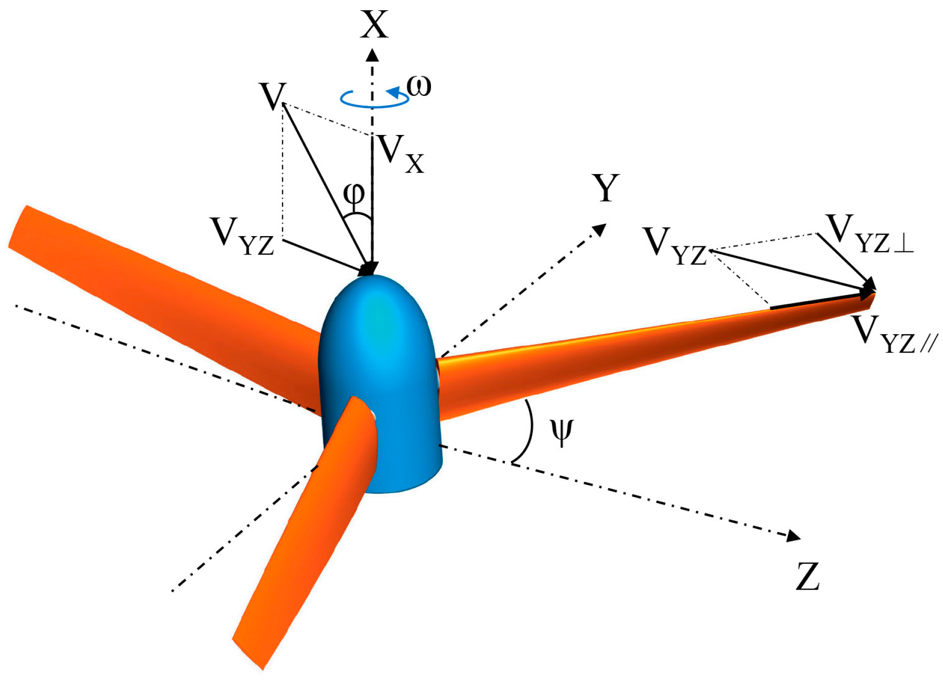
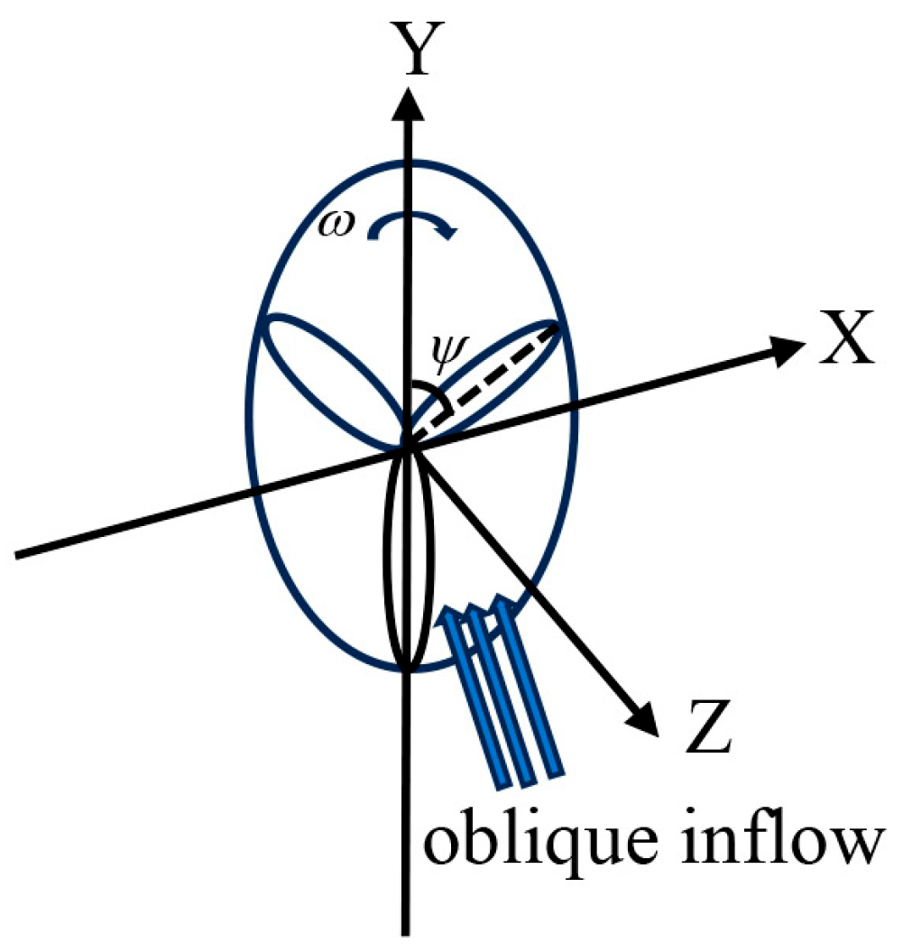
Figure 2 shows the coordinate system of each velocity component of the propeller, where the direction perpendicular to the direction of the propeller disc is considered as the X-axis. In addition, the plane in which the propeller disc is located is defined as the YZ-plane, and φ denotes the angle between the inflow velocity V and the X-axis of the rotational axis of the propeller disc. Therefore, the incoming velocity V can be decomposed into the axial component VX and the tangential component of the propeller disc VYZ, given in Equations (9) and (10), respectively.
A further decomposition of the tangential component VYZ yields VYZ⊥ perpendicular to the leading edge of the blade and VYZ∥ parallel to the radial direction of the blade:
where ψ denotes the azimuth angle of the propeller blade.
According to the blade element theory, the lift resistance and the relative velocity produced by the blade element are shown in Figure 3. In Figure 3, α is the angle of attack, β is the propeller blade angle, ϕ is the airflow angle, and ω is the angular velocity. The expression for the relative velocity VR produced by the airflow relative to the blade element is:
where Via denotes the axial induced velocity of each segment of the propeller blade, dL denotes the instantaneous lift perpendicular to the relative velocity VR, and dD denotes the drag along VR.
The instantaneous thrust force generated by the blades of the propeller is different at different moments during the rotation cycle due to the different azimuth angles at which the blades are located. But the average thrust force generated by the blades is the same. For N propeller blades, the average thrust force and the torque generated by the rotation for one cycle are:
where CL is the lift coefficient, CD is the drag coefficient, b is the chord length, and r is the radius of the propeller at any position.
Based on momentum theory along with Bernoulli’s equation and the conservation of momentum theorem, thrust and torque equations are obtained as follows:
where Vdisc denotes the resultant flow velocity through the propeller. This velocity varies with azimuth, and can be expressed as:
In the case of zero inflow angle, the resulting equations (i.e., Equations (13)–(16)) can be solved by means of iterative solution. This is because the unknown axial induced velocity Via is constant for the same position of the blade, and thus the joint Equations (13)–(16) can only be solved by means of iterative algorithms. But, otherwise, the axial induced velocity Via is a function of the azimuth angle. Therefore, it is necessary to introduce the inlet model developed by Peters and Pitt [23,24] to describe the relationship between the induced velocity Via and the azimuth angle. The expression according to this model is:
where Via,0 is the induced velocity at the center of the propeller on the propeller plane, and R denotes the total radius of the propeller. Figure 4 is a schematic diagram of the propeller wake deflection, χ is the wake skew angle given by:
The tangential force is given by:
The bending moment is given by:
To determine the unknown induced velocities Via,0, Equations (18) and (19) are first substituted into Equations (12)–(16). Then, Equations (13)–(16) are joined and solved iteratively for unknowns. Subsequently, the thrust force dT and the overcoming torque dQ are determined. The above calculation steps can then be repeated for each position of blade extension, and the thrust force dT and the torque dQ can be integrated to obtain the aerodynamic performance parameters of the propeller in the case of an inflow angle.
By making the aerodynamic parameters of the propeller dimensionless, the following equations are obtained:
Thrust coefficient CT:
Power coefficient CP:
Tangential force coefficient CF:
Bending moment coefficient CB:
where D is the diameter of the propeller.
2.2. Mathematical Model Correction
2.2.1. Tip Correction
The Prandtl tip correction model, which was introduced in reference [9], is used to simulate the phenomenon of lift reduction to zero at the tip of the propeller. The reason for this phenomenon is that there is no barrier on the outside of the blade tip. The tip airfoil accelerates the airflow over the upper airfoil, thereby increasing the static pressure difference with the lower airfoil. But the airflow escapes from the lower airfoil to the upper airfoil along the tip, creating a tip vortex and a static pressure difference. This is the reason why there is a sudden drop in tip lift. This phenomenon also spreads to some blade elements near the tip of the propeller and the degree of lift attenuation is greatly increased. The Prandtl tip correction model describes the distribution of the correction coefficient Fprandtl at the propeller blade spanwise.
where N denotes the number of propeller blades, φ denotes the inlet angle of the airfoil, R denotes the complete radius of the propeller, and r denotes the radius of the propeller at any position.
2.2.2. Root Flow Correction
When the propeller moves, the fluid is influenced especially near the root of the propeller. Flow separation at the root of the propeller means the loss of connection between the fluid and the impeller in this area. Flow separation at the root of the propeller can lead to performance issues such as reduced efficiency, increased noise, and vibration. A possible cause of this phenomenon may be that the propeller, under the conditions of oblique inflow, experiences excessive angles of attack. This may lead to the inability of the fluid to properly adhere to the surface of the blade, resulting in separation at the root of the propeller.
To accurately simulate such a flow separation phenomenon, the main correction was carried out at the propeller root. According to our research experiences, it is suggested to define a function Fcl as follows:
where r denotes the radius at any position of the propeller. Figure 5 is a function diagram of Fcl. The horizontal coordinate represents the position of blade extension (r/R), and the longitudinal coordinate is the function value of the corresponding position. The value of the function closer to the root is smaller, the corresponding correction at the root of the propeller is larger, the value of the function closer to the tip is closer to 1, and the correction at the tip is smaller.
The corrected lift coefficients (CL correct) are then obtained by multiplying both Fprandtl and Fcl by the corresponding wing lift coefficients (CL). All subsequent calculations will be performed using the corrected lift coefficients.
2.3. Implementation of Calculation Method Based on MATLAB
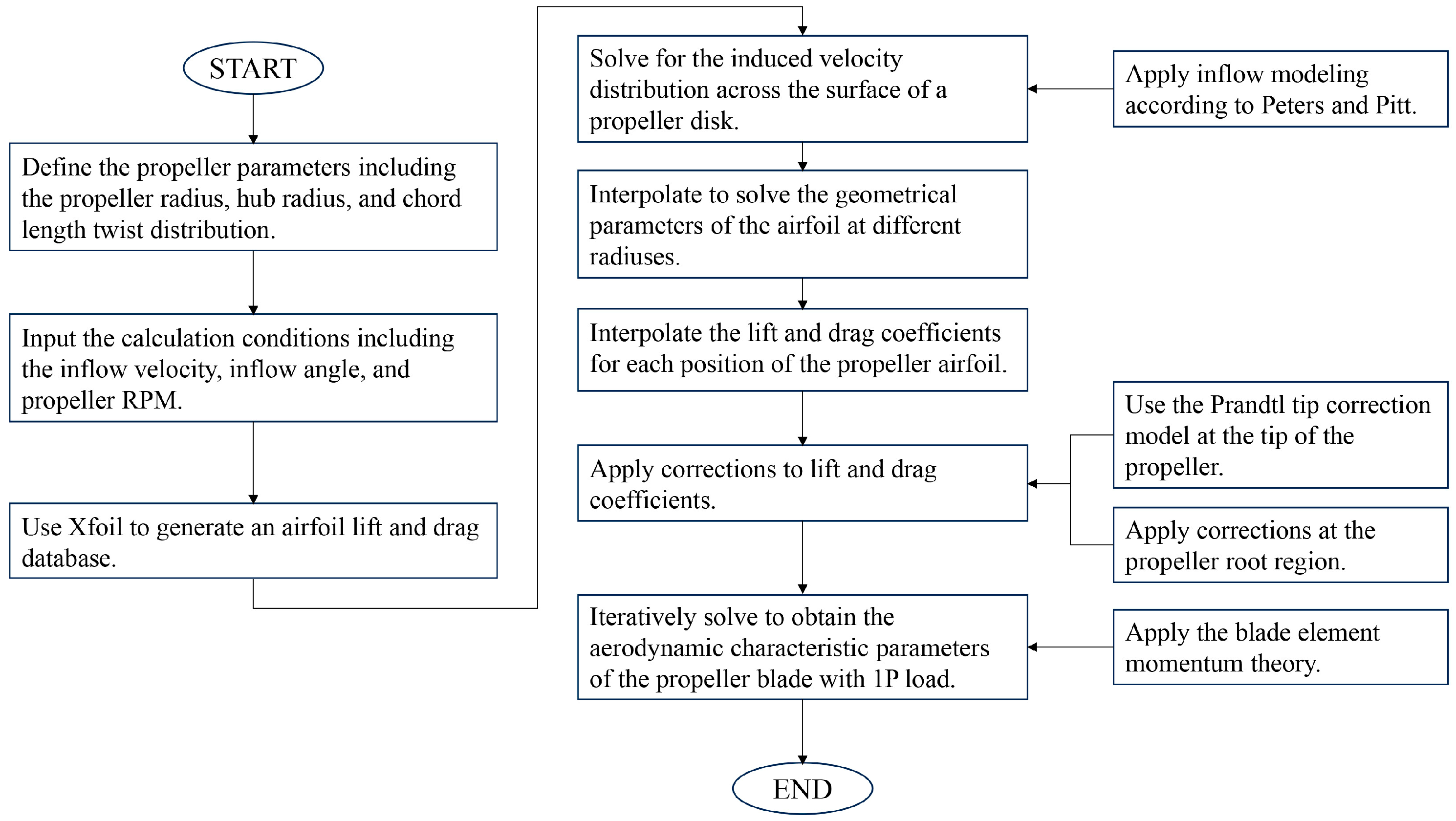
The procedure for calculating the propeller 1P load is described in Figure 6. In the first step, we start by defining the basic parameters of the propeller such as the number of propeller blades, radius, hub radius, blade chord length, and twist distribution. In the second step, the calculation conditions such as inflow angle, inflow velocity, and other operating conditions are specified. In the third step, Xfoil V6.94 is used to generate a database of lift and drag coefficients for the airfoil and import them into the MATLAB procedure. Next, the inflow model established by Peters and Pitt is introduced and the resulting equations are solved iteratively for the induced velocity distribution on the propeller disc. In the fifth step, the interpolation of the solution gives parameters such as chord length and blade angle at any radius of the propeller blade. Next, the lift drag coefficients are called from the database and interpolated to solve for the lift drag coefficients at each position of the propeller airfoil. Then, the Prandtl tip correction model is applied to correct at the propeller blade tip, and also correct at the propeller root based on Fcl due to separation flow at the root. The correction coefficients at different radii are multiplied by the corresponding lift coefficients to obtain the corrected lift coefficients. In the final step, the inflow velocity is decomposed and iteratively solved for aerodynamic performance parameters such as propeller blade bending moment and tangential force based on the blade element momentum theory.
3. Validation of the CFD Calculation Method
To validate the accuracy and reliability of the proposed procedure, a CFD simulation is also conducted for the propeller. The results of the proposed procedure are then compared with the CFD simulation results to verify the accuracy of the developed procedure.
Based on Equation (30), the Reynolds number is in the range of 3 × 10⁵–5 × 10⁵ from root to tip. This is a typical turbulent flow, and the turbulence model is introduced to CFD calculations.
In Equation (30), U is the fluid velocity, L is the characteristic length, and μ is the fluid viscosity.
The flow of the fluid is assumed to be governed by the Favre-averaged Navier–Stokes (N-S) equations. In the Cartesian coordinate system, the differential forms of the continuity equation, momentum equation, and energy equation are given by:
where u, p, ρ, E, τ, t, xi, and qi are velocity, pressure, density, total energy, stress, time, spatial coordinates, and heat flux, respectively. Furthermore, δij is the Kronecker symbol that is 1 when i = j and 0 otherwise.
The turbulence model used in this paper is the two-equation SST k-ω model. The SST k-ω model is a combination of k-ω and k-ε models. The k-ω model is used in the near-wall boundary layer region, which does not require the wall attenuation function and does not produce rigidity in the numerical solution. Also, it has the Reynolds shear stress transport property in the inner layer of the boundary layer. On the other hand, the k-ε model is used in the region outside the boundary layer, which is able to provide a better adaptation to the free shear flow. The model is described by the following differential equations:
where Ω is the vorticity. In addition, F1 and F2 are mixing functions, related to the distance from the point to the wall, where the role of the mixing function F1 is to complete the transition from the k-ω model near the wall to the k-ε model far from the wall. More details can be found in references [25,26].
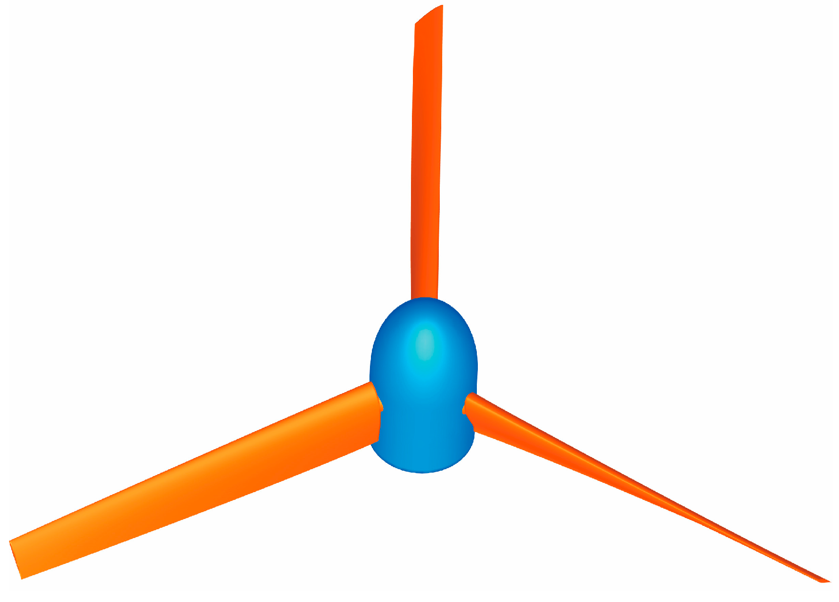
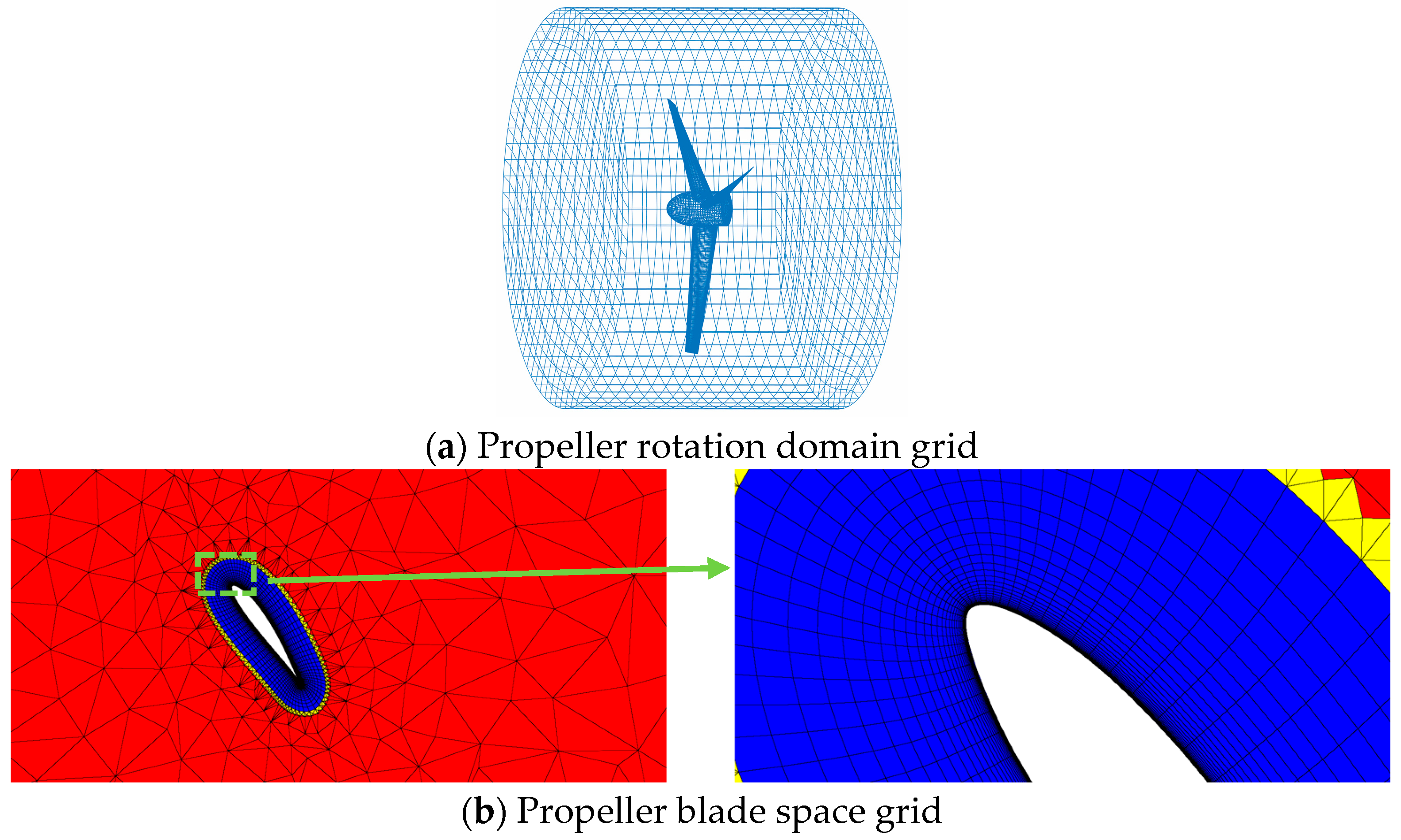
The propeller model used in this paper is shown in Figure 7. The model includes a three-bladed propeller with a propeller radius of 0.525 m, a hub radius of 0.606 m, and a pitch angle of 56° at the 70% radius position. Figure 8 shows the grid of propeller. The geometric model of the propeller is meshed using Pointwise V18.5R1 software based on the unstructured mesh generation method. Also, the T-Rex technique was used to generate a high-quality boundary layer mesh with a maximum Y+ less than 1.0 near the wall. The computational domain was divided into two parts: the inner part, which is the rotating region with the propeller, and the outer part, which is the non-rotating constant far-field region. CFD numerical calculations were performed using Ansys CFX software version 19.1 [27], based on the slip mesh method, with an interface between the rotating and non-rotating regions for the interpolation and exchange of data, using the transient rotor-stator setup method and the convective terms in high-resolution scheme. Boundary conditions included inflow conditions, far-field conditions, and solid-wall boundary conditions. Inlet conditions were determined based on flight altitude and velocity, considering total temperature and total pressure. The inflow direction made an angle with the inlet boundary. Far-field boundary conditions were set as open, with the turbulence intensity set to zero gradient. The propeller blades and hub were set as no-slip adiabatic wall conditions, and the initial field was set as a uniform inflow.
In order to minimize the influence of the mesh on the computational results, the mesh-independence of the propeller was first verified. Three different sets of grids were generated with 0.89 million, 1.36 million, and 2.71 million grids. Figure 9 shows the variation in power coefficients with rotational speed for different grids. It can be seen from Figure 9 that the calculation results with different grids are basically consistent at low RPM. However, as the speed increases, some slight differences are observed between the calculated results. Also, at a constant rotational speed, the power coefficient decreases with the increase in the grid number. When the number of grids reaches 2.71 million, the calculation results are almost the same as the 1.36 million grids, which indicates that the 1.36 million grids have reached the grid-independence requirements. Thus, the grid number 1.36 million is subsequently used for the calculation, taking into account the calculation time and calculation efficiency.
In this paper, wind tunnel experiments were used to verify the accuracy of the CFD method. The tests were based on a single-rotor propeller test platform in a low-speed wind tunnel. The test equipment was placed in the air outlet of the wind tunnel. The absolute pressure of the experimental environment was 103,474 pa, the density of air was 1.17 kg/m3, and the inflow wind speed was set at 82 m/s. In addition, the diameter of the rotor propeller was 1.05m. The experimental data are shown in Table 1.
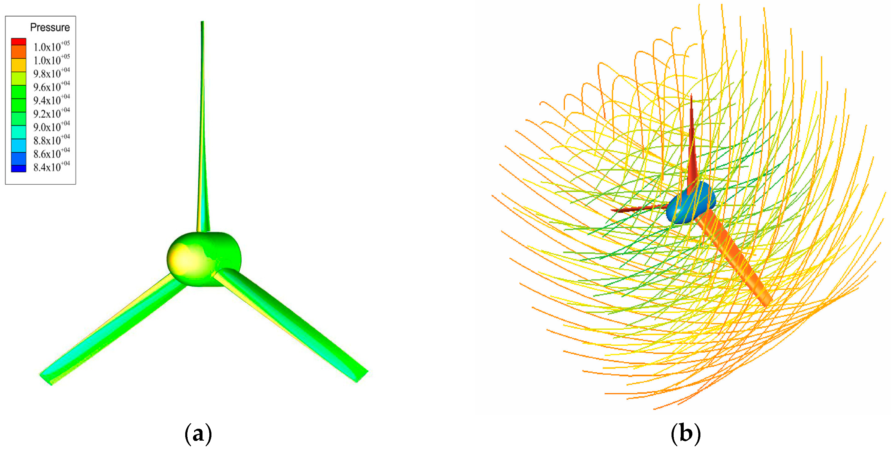
Figure 10 shows the variation in thrust coefficient CT and power coefficient CP with propeller speed for axial incoming flow, in which “Exp.” represents the experimental value while “Cal.” represents the CFD calculated value. It can be seen that the calculated and experimental values are relatively close to each other. The average error of CT is 5.50%, while that of CP is 6.80%. Since the accuracy of the CFD simulation results is very good, they can be used to validate the results of the procedure developed in this paper. Figure 11 shows the static pressure contour and the streamline distribution of the propeller under the conditions of a rotational speed of 1396.9 min−1, and an axial inflow speed of 82 m/s. From Figure 11, one can see the distribution characteristics of the low-pressure area of the suction surface and the high-pressure area of the pressure surface as well as the characteristics of the streamline distribution in the vicinity of the propeller.
4. Analysis of Calculation Results
The propeller 1P loads were calculated at different inflow angles to verify the accuracy of the procedure using the CFD calculation data as a reference. The thrust coefficient (CT), power coefficient (CP), blade bending moment coefficient (CB), and tangential force coefficient (CF) of individual propeller blades were calculated for inflow angles of 9°, 12°, and 15° to characterize the load distribution of each blade of the propeller and the aerodynamic performance of the whole propeller with blade azimuthal angle. The equation for calculating the deviation between the CFD calculation results and the procedure calculation results is as follows:
where e represents the deviation between the results of the proposed procedure and the CFD simulation results, and WPro. represents the value calculated using the proposed procedure, including CB Pro., which represents the bending moment coefficient calculated using the proposed procedure; CF Pro., which represents the tangential force coefficient calculated using the proposed procedure; CT Pro., which represents the thrust coefficient calculated using the proposed procedure; and CP Pro., which represents the power coefficient calculated using the proposed procedure. Furthermore, WCal. represents the value calculated using the CFD simulation, including CB Cal., which represents the bending moment coefficient calculated using CFD simulation; CF Cal., which represents the tangential force coefficient calculated using CFD simulation; CT Cal., which represents the thrust coefficient calculated using CFD simulation; and CP Cal., which represents the power coefficient calculated using CFD simulation. In addition, M represents the amount of pulsation of the CFD calculated value, i.e., the difference between the peaks and troughs of the CFD calculated value.
Figure 12 shows a schematic diagram of the direction of propeller rotation (ω), the relative position of the propeller blades, and the azimuth angle (ψ) in the CFD numerical calculation.
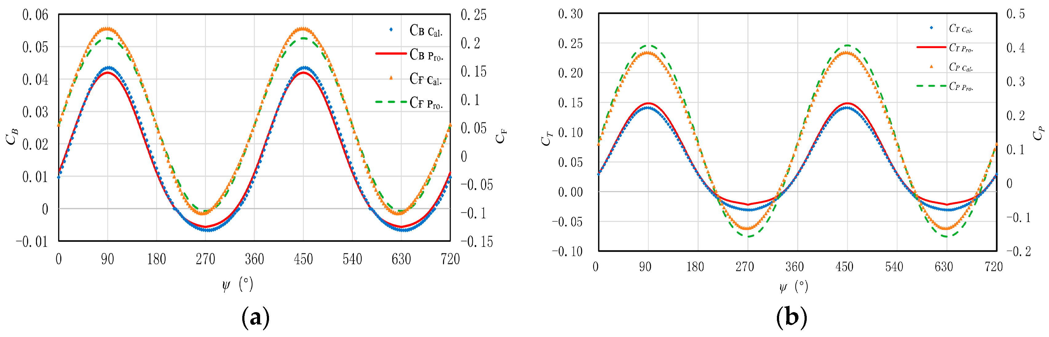
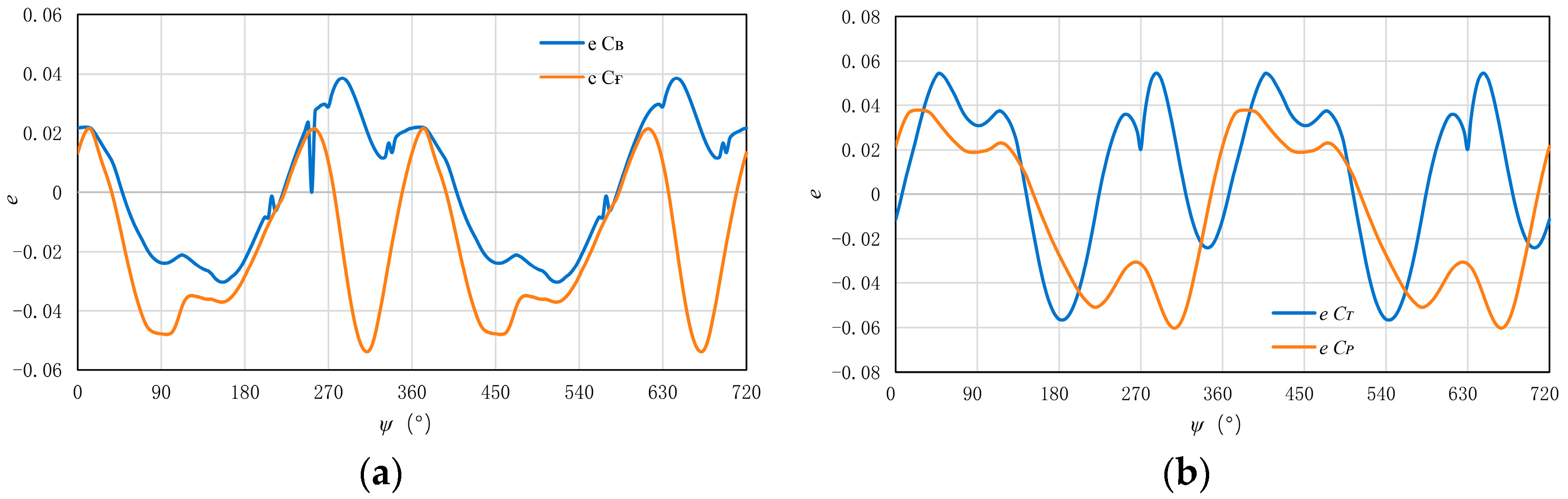
Figure 13 shows a comparison between the results of the proposed procedure and the values calculated using the CFD simulation for a propeller blade with an inflow angle of 9°. It can be seen that in the case of oblique inflow, the aerodynamic parameters of individual blades of the propeller show regular pulsating periodic changes with blade azimuthal angle. Also, the maximum value of the 1P load occurs near 90° while the minimum value occurs near 270°, which is in line with the actual force situation of the propeller. In addition, the predicted values of the procedure are close to the CFD calculated values. Figure 14 shows the variation in the deviation (defined in Equation (37)) with azimuth. We found that the maximum deviation of the CB is −2.30%, the maximum deviation of the CF is −4.85%, the maximum deviation of the CT is 5.00%, and the maximum deviation of the CP is −4.50% during one cycle of propeller blade rotation. This implies that the error value of the proposed procedure is in a small range. In addition, the peak valley pattern predicted using the proposed procedure is also very consistent with the CFD calculation results, indicating that the mathematical model proposed in this paper can well reflect the actual physical flow of the propeller.
Figure 15 shows a comparison between the results of the proposed procedure and those of CFD simulation for an inflow angle of 12°. Figure 16 shows the variation in the deviation with azimuth. It is found that the maximum deviation of CB during one propeller rotation cycle is −3.89%, the maximum deviation of CF is −5.56%, the maximum deviation of CT is 6.00%, and the maximum deviation of CP is −5.70%, all of which are relatively small deviations. Moreover, the change rule of the 1P load here is the same as that of the inflow angle of 9°, but the pulsation of the aerodynamic parameters of the propeller increases.
Figure 17 shows a comparison of the results when the inflow angle is 15°. Figure 18 shows the variation in the deviation with azimuth. In this case, the maximum deviation of the CB during one circle of propeller rotation is 3.90%, the maximum deviation of the CF is −5.40%, the maximum deviation of the CT is −5.70%, and the maximum deviation of the CP is −6.00%. The 1P load also shows a periodic variation, which increases in magnitude in comparison to the flow angle of 12° and 9°.
To compare the results of the proposed method with the results of the CFD simulation, the values of CB and CF of the whole propeller were calculated for different angles of the inflow, and the results are shown in Figure 19. It is noted that to study the effect of 1P aerodynamic load on the whole propeller, we have to consider three blades together. Figure 19a–c show the results for the CB and CF of the entire propeller at different inflow angles of 9°, 12°, and 15°, respectively. It can be seen that the results of the proposed method are in good agreement with the CFD simulation results, and, as expected, the results of CB are in better agreement. On the other hand, it is observed that the total bending moment and the total tangential force increase with the increase in the inflow angle.
The above results clearly show the accuracy of the proposed procedure, which was also found to have the advantages of being fast and efficient throughout the study. Under the condition of using the computing node configuration of Intel (R) Xeon (R) Platinum 9242 CPU @ 2.30 GHz with 90 supercomputer cores, it takes about 6h to calculate a certain working condition of an unsteady propeller flow by means of CFD simulation. This is not only slow, but also computationally expensive and requires a great deal of configuration of the operating environment. But the time required to calculate the same working condition of the propeller by means of the proposed procedure is <1 s, which has high computational efficiency and requires less operating environment.
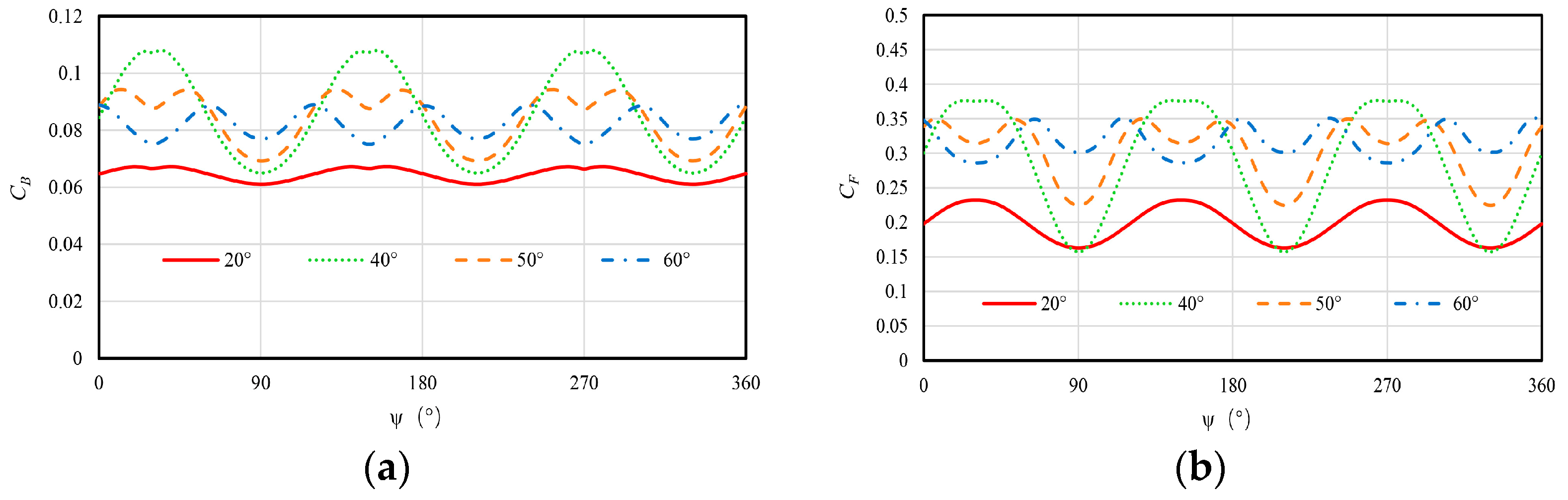
The calculation results in Figure 13, Figure 14, Figure 15, Figure 16, Figure 17, Figure 18 and Figure 19 also confirm the accuracy and reliability of the proposed method. Next, the procedure was used to calculate the variation in the CB and CF of the whole propeller with the azimuthal angle of the blade at larger inflow angles. In addition, the distribution of the CB and CF of the whole propeller was further studied under different advance ratios. Figure 20 shows the variation in the CB and CF of the whole propeller with blade azimuthal angle for large inflow angles of the propeller (20°, 40°, 50°, and 60°). It can be seen from Figure 20 that the range of fluctuations in the CB and CF of the propeller first increases and then decreases from the inflow angle of 20° to the inflow angle of 60°. Also, they all have clear variation patterns with different inflow angles. This is because in the case of a small inflow angle, the fluid flows through the propeller at a lower speed on the rotating surface of the propeller, which results in a lower bending moment and tangential force. Also, as the inflow angle increases, more force is required to push the fluid. But when the inflow angle is too large, it leads to severe separation and fluid stagnation, which then reduces the overall propeller bending moment and tangential force. On the other hand, in the case of a large inflow angle, the fluid forms non-uniform flows near the propeller. These irregular flows then cause the propeller to be subjected to highly unstable forces, which result in irregular fluctuations.
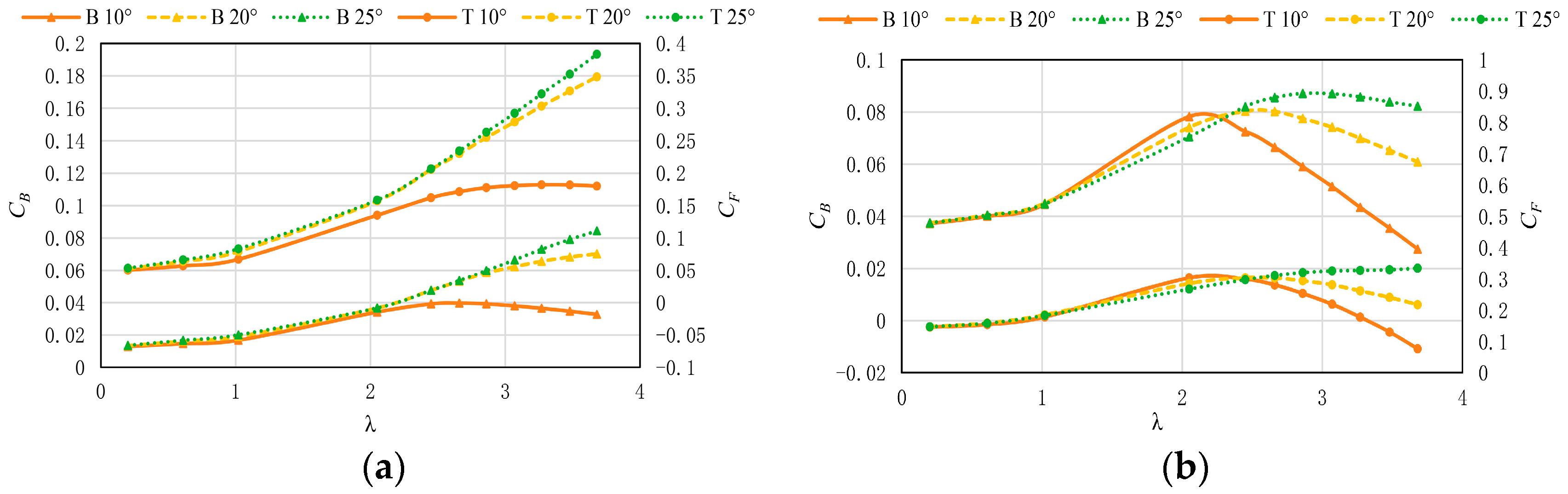
Figure 21a shows the variation in maximum CB and CF of an individual propeller blade at a rotational speed of 1396.9 min−1, inflow angles of 10°, 20°, and 25°, and different advance ratios of the propeller. In the case of an inflow angle of 10°, the maximum CB occurs on a blade with an advance ratio of about 2.5, the CF suffered by a blade does not greatly change with the increase in the advance ratio after it reaches 150N, and the value is relatively stable. When the inflow angle is 20° or 25°, the maximum CB and the maximum CF of a blade increase with the increase in the propeller advance ratio. In addition, a larger inflow angle corresponds to a larger CB and CF, which is in line with the basic working characteristics of the propeller. The greater the angle of inflow, the greater the 1P aerodynamic load on the propeller and the more unfavorable it is for the performance of the propeller. Figure 21b shows the variation in the maximum CB and maximum CF of the whole propeller with advance ratio. It can be seen that in the range of advance ratios calculated in this paper, there is an extreme value of the maximum CB and maximum CF of the whole propeller for inflow angles of 10° and 20°. This extreme value of the 1P load is the most unfavorable factor for the propeller. When the inflow angle is 25°, the CB will remain basically unchanged after reaching a certain value, and the CF will slightly increase with the increase in the advance ratio. This also indicates that a larger inflow angle will lead to a more complicated flow and more severe propeller working conditions. Through the analysis of 1P aerodynamic loads of a single blade and the whole propeller, it can be seen that the procedure developed in this paper can effectively predict the maximum bending moment and tangential force of the propeller blade. Therefore, the proposed procedure is expected to provide some guidance for the strength design of propeller structures.
5. Conclusions
In this paper, a mathematical model of propeller 1P aerodynamic loads was established based on the theory of blade element momentum, and a fast calculation procedure of propeller 1P aerodynamic loads was developed. According to the presented results, the following conclusions can be drawn:
- (1)
- Under conditions of non-axial inflow, the flow field surrounding the propeller becomes even more complex, thereby posing substantial challenges in accurately and efficiently predicting its aerodynamic performance. The implement of the inflow model proposed by Peters and Pitt, in conjunction with Prandtl’s blade tip correction and our novel propeller root flow correction method, has significantly enhanced the precision of the blade element momentum theory in predicting the aerodynamic loads of the propeller.
- (2)
- By comparing the results of the proposed procedure with those of the CFD simulation at different inflow angles, it was found that the deviation of the results of the proposed method and CFD simulation results for the blade aerodynamic characteristic parameters is in a small range of ±6.00%. This confirms the applicability and accuracy of the proposed procedure for predicting the propeller 1P loads. On the other hand, the proposed procedure has the advantage of low computational cost, and is therefore an efficient method to calculate the propeller 1P loads.
- (3)
- Through the calculation of the propeller 1P loads, the variation in propeller CB and CF with the blade azimuth angle was studied. It was found that the values of the aerodynamic characteristic parameters of the individual propeller blade show obvious periodic changes with azimuth angle. Also, the maximum value of the individual propeller blade 1P load occurs near 90° while the minimum value occurs near 270°. In addition, the overall aerodynamic characteristic parameter of the propeller fluctuates with the inflow angle in a certain range, the fluctuation is also smaller, and as the angle of inflow increases, the fluctuation is more complex.
- (4)
- Through the analysis of the calculation results of the maximum CB and CF of the propeller blade with the variation in advance ratio, it was found that the calculation procedure developed herein can effectively predict the maximum bending moment and tangential force of the propeller blade. It is expected that this method can provide a certain guidance for the successful design and reliable operation of propellers.
Author Contributions
W.Y.: Writing—original draft, Supervision, Methodology, Conceptualization, and Programing the new procedure. X.T.: Writing—original draft, Data curation, and Running calculations with the new procedure. J.Z.: Writing—original draft, Supervision, Methodology, Conceptualization, and Programing the new procedure. K.Z.: Writing—review and editing, and Performing the CFD calculations. All authors have read and agreed to the published version of the manuscript.
Funding
This research was funded by the Advanced Aircraft Engine Project Foundation (Grant number: HKCX2020-02-024 and HKCX2024-01-023).
Data Availability Statement
Data is contained within the article.
Acknowledgments
The authors would like to acknowledge Yang Xiao from the Institute for Aero Engine of Tsinghua University.
Conflicts of Interest
The authors declare no conflicts of interest.
References
- Qu, Y.C.; Zhang, Y.F.; Song, W.G. Flight test study of propeller 1P moment. Flight Mech. 2007, 25, 68–71. [Google Scholar]
- Liu, X.; Liu, P.Q.; Sun, T.; Wang, H.Y.; Hu, T.X. Aerodynamic and noise characteristics of civil aircraft propellers under 1P load. In Proceedings of the Professional Committee of Fluid Mechanics, Chinese Society of Mechanics, Abstracts of the 12th National Academic Conference on Fluid Mechanics. Lu Shijia Laboratory, Beijing University of Aeronautics and Astronautics (Key Laboratory of Aero-Aerodynamic Acoustics, Ministry of Industry and Information Technology). Xi’an, China, 22–25 September 2022. [Google Scholar]
- Gonzalez-Martino, I.; François, B.; Rodriguez, B. A numerical insight into contra-rotating open rotor in-plane loads. Mech. Ind. 2014, 15, 19–28. [Google Scholar] [CrossRef]
- Kim, C.J.; Kim, S.H.; Park, T.; Park, S.H.; Lee, J.W.; Ko, J.S. Flight Dynamics Analyses of a Propeller-Driven Airplane (I): Aerodynamic and Inertial Modeling of the Propeller. Int. J. Aeronaut. Space Sci. 2014, 15, 345–355. [Google Scholar] [CrossRef]
- Dorfling, J.; Rokhsaz, K. Integration of Airfoil Stall and Compressibility Models into a Propeller Blade Element Model. J. Aerosp. Eng. 2016, 29, 04016014. [Google Scholar] [CrossRef]
- Kolaei, A.; Barcelos, D.; Bramesfeld, G. Experimental Analysis of a Small-Scale Rotor at Various Inflow Angles. Int. J. Aerosp. Eng. 2018, 2018, 2560370. [Google Scholar] [CrossRef]
- Theys, B.; Dimitriadis, G.; Andrianne, T.; Hendrick, P.; De Schutter, J. Wind tunnel testing of a VTOL MAV propeller in tilted operating mode. In Proceedings of the International Conference on Unmanned Aircraft Systems, Orlando, FL, USA, 27–30 May 2014; IEEE: Piscataway, NJ, USA, 2014. [Google Scholar]
- Zarev, A.; Green, R. Experimental investigation of the effect of yaw angle on the inflow of a two-bladed propeller. Aerosp. Sci. Technol. 2020, 103, 105940. [Google Scholar] [CrossRef]
- Higgins, R.; Zarev, A.; Barakos, G.; Green, R.B. Numerical Investigation of a Two-Bladed Propeller Inflow at Yaw. J. Aircr. 2020, 57, 292–304. [Google Scholar] [CrossRef]
- Cerny, M.; Breitsamter, C. A Comparison of Isolated and Ducted Fixed-Pitch Propellers Under Non-Axial Inflow Conditions. Aerospace 2020, 7, 112. [Google Scholar] [CrossRef]
- Park, D.; Lee, Y.; Cho, T.; Kim, C. Design and Performance Evaluation of Propeller for Solar-Powered High-Altitude Long-Endurance Unmanned Aerial Vehicle. Int. J. Aerosp. Eng. 2018, 2018 Pt 2, 5782017. [Google Scholar] [CrossRef]
- Garcia, A.J.; Barakos, G.N. Numerical simulations on the ERICA tiltrotor. Aerosp. Sci. Technol. 2017, 64, 171–191. [Google Scholar] [CrossRef]
- Brandt, J.B.; Selig, M.S. Propeller Performance Data at Low Reynolds Numbers. In Proceedings of the 49th AIAA Aerospace Sciences Meeting including the New Horizons Forum and Aerospace Exposition, Orlando, FL, USA, 4–7 January 2011. [Google Scholar]
- Silvestre, M.A.; Morgado, J.P.; Páscoa, J. JBLADE: A propeller design and analysis code. In Proceedings of the International Powered Lift Conference, Los Angeles, CA, USA, 12–14 August 2013. [Google Scholar]
- Mccrink, M.H.; Gregory, J.W. Blade Element Momentum Modeling of Low-Reynolds Electric Propulsion Systems. J. Aircr. 2016, 54, 163–176. [Google Scholar] [CrossRef]
- Khan, W.; Nahon, M. A propeller model for general forward flight conditions. Int. J. Intell. Unmanned Syst. 2015, 3, 72–92. [Google Scholar] [CrossRef]
- Yang, X.; Wang, X.; Zhu, J.; Yan, W. Modelling, analysis and experimental study of the prop-rotor of vertical/short-take-off and landing aircraft. Proc. Inst. Mech. Eng. Part G J. Aerosp. Eng. 2022, 236, 2885–2908. [Google Scholar] [CrossRef]
- Zhang, Y.F.; Zhang, Q.; Ren, R.D. Study on propeller shaft test for 1P load flight test of propeller. Flight Mech. 2011, 29, 84–88. [Google Scholar]
- The MathWorks Inc. MATLAB 9.12.0 (R2022a), The MathWorks Inc.: Natick, MA, USA, 2022.
- Liu, P.Q. Air Propeller Theory and Its Applications; Beijing University of Aeronautics and Astronautics Press: Beijing, China, 2005. [Google Scholar]
- Seddon, J.; Newman, S. Basic Helicopter Aerodynamics; National Defense Industry Press: Beijing, China, 2014. [Google Scholar]
- Wang, S.C.; Xu, G.H. Development of helicopter rotor aerodynamics. J. Nanjing Univ. Aeronaut. Astronaut. 2001, 33, 0203–0211. [Google Scholar]
- Pitt, D.M.; Peters, D.A. Theoretical prediction of dynamic inflow derivatives. Vertica 1981, 47, 1–18. [Google Scholar]
- Chen, R.T.N. A survey of nonuniform inflow models for rotorcraft flight dynamics and control applications. In Proceedings of the European Rotorcraft Forum, Amsterdam, The Netherlands, 12–15 September 1989. [Google Scholar]
- Menter, F.R. Two-equation eddy-viscosity turbulence models for engineering applications. AIAA J. 1994, 32, 1598–1605. [Google Scholar] [CrossRef]
- Menter, F. Zonal two equation k-w turbulence models for aerodynamic flows. In Proceedings of the 24th Fluid Dynamics Conference, Orlando, FL, USA, 6–9 July 1993. [Google Scholar]
- ANSYS. CFX-Pre User’s Guide; Release 19.1; ANSYS, Inc.: Canonsburg, PA, USA, 2018. [Google Scholar]
Figure 1.
BEM theoretical velocity diagram.

Figure 2.
Definition of the propeller coordinate system and decomposition of the incoming velocity.

Figure 3.
Blade element force diagram.

Figure 4.
Propeller wake deflection.

Figure 5.
Variation in Fcl with r/R.

Figure 6.
Flowchart of calculation procedure for propeller 1P load.

Figure 7.
Geometry of the propeller model.

Figure 8.
Propeller grid.

Figure 9.
Variation in CP with propeller rotation speed for different grid numbers.

Figure 10.
Variation in propeller CT and CP with rotational speed at zero inflow angle.

Figure 11.
Propeller pressure contour plot and streamline distribution: (a) propeller pressure contour; (b) propeller streamline distribution.
Figure 11.
Propeller pressure contour plot and streamline distribution: (a) propeller pressure contour; (b) propeller streamline distribution.

Figure 12.
Schematic diagram of the azimuthal angle.

Figure 13.
Variation in propeller aerodynamic parameters with azimuth at an inflow angle of 9°: (a) CB and CF; (b) CT and CP.
Figure 13.
Variation in propeller aerodynamic parameters with azimuth at an inflow angle of 9°: (a) CB and CF; (b) CT and CP.

Figure 14.
Variation in the deviation with azimuth at an inflow angle of 9°: (a) e CB and e CF; (b) e CT and e CP.
Figure 14.
Variation in the deviation with azimuth at an inflow angle of 9°: (a) e CB and e CF; (b) e CT and e CP.

Figure 15.
Variation in propeller aerodynamic parameters with azimuth at an inflow angle of 12°: (a) CB and CF; (b) CT and CP.
Figure 15.
Variation in propeller aerodynamic parameters with azimuth at an inflow angle of 12°: (a) CB and CF; (b) CT and CP.

Figure 16.
Variation in the deviation with azimuth at an inflow angle of 12°: (a) e CB and e CF; (b) e CT and e CP.
Figure 16.
Variation in the deviation with azimuth at an inflow angle of 12°: (a) e CB and e CF; (b) e CT and e CP.

Figure 17.
Variation in propeller aerodynamic parameters with azimuth at an inflow angle of 15°: (a) CB and CF; (b) CT and CP.
Figure 17.
Variation in propeller aerodynamic parameters with azimuth at an inflow angle of 15°: (a) CB and CF; (b) CT and CP.

Figure 18.
Variation in the deviation with azimuth at an inflow angle of 15°: (a) e CB and e CF; (b) e CT and e CP.
Figure 18.
Variation in the deviation with azimuth at an inflow angle of 15°: (a) e CB and e CF; (b) e CT and e CP.

Figure 19.
Variation in CB and CF of the whole propeller with azimuth for different inflow angles: (a) CB and CF at an inflow angle of 9°; (b) CB and CF at an inflow angle of 12°; and (c) CB and CF at an inflow angle of 15°.
Figure 19.
Variation in CB and CF of the whole propeller with azimuth for different inflow angles: (a) CB and CF at an inflow angle of 9°; (b) CB and CF at an inflow angle of 12°; and (c) CB and CF at an inflow angle of 15°.

Figure 20.
CB and CF of the whole propeller at different inflow angles: (a) CB of the whole propeller; (b) CF of the whole propeller.
Figure 20.
CB and CF of the whole propeller at different inflow angles: (a) CB of the whole propeller; (b) CF of the whole propeller.

Figure 21.
Variation in CB and CF with advance ratio: (a) variation in CB and CF of single-blade propeller with advance ratio; (b)variation in CB and CF of three-blade propeller with advance ratio.
Figure 21.
Variation in CB and CF with advance ratio: (a) variation in CB and CF of single-blade propeller with advance ratio; (b)variation in CB and CF of three-blade propeller with advance ratio.


Table 1.
Experimental values of CT and CP.
| RPM | CT | CP |
|---|---|---|
| 1309.7 | 0.0340 | 0.2623 |
| 1396.9 | 0.0661 | 0.3441 |
| 1496.8 | 0.0995 | 0.4053 |
| 1602.6 | 0.1297 | 0.4443 |
| 1694.3 | 0.1511 | 0.4705 |
| 1797.3 | 0.1704 | 0.4956 |
Disclaimer/Publisher’s Note: The statements, opinions and data contained in all publications are solely those of the individual author(s) and contributor(s) and not of MDPI and/or the editor(s). MDPI and/or the editor(s) disclaim responsibility for any injury to people or property resulting from any ideas, methods, instructions or products referred to in the content. |
© 2024 by the authors. Licensee MDPI, Basel, Switzerland. This article is an open access article distributed under the terms and conditions of the Creative Commons Attribution (CC BY) license (https://creativecommons.org/licenses/by/4.0/).
Share and Cite
MDPI and ACS Style
Yan, W.; Tian, X.; Zhou, J.; Zhang, K. Research on the Calculation Method of Propeller 1P Loads Based on the Blade Element Momentum Theory. Aerospace 2024, 11, 332. https://doi.org/10.3390/aerospace11050332
AMA Style
Yan W, Tian X, Zhou J, Zhang K. Research on the Calculation Method of Propeller 1P Loads Based on the Blade Element Momentum Theory. Aerospace. 2024; 11(5):332. https://doi.org/10.3390/aerospace11050332
Chicago/Turabian StyleYan, Wenhui, Xiao Tian, Junwei Zhou, and Kun Zhang. 2024. "Research on the Calculation Method of Propeller 1P Loads Based on the Blade Element Momentum Theory" Aerospace 11, no. 5: 332. https://doi.org/10.3390/aerospace11050332
Note that from the first issue of 2016, this journal uses article numbers instead of page numbers. See further details here.