Article

Multi-Model Projections of River Flood Risk in Europe under Global Warming

1
European Commission—Joint Research Centre, 21027 Ispra, Italy
2
College of Life and Environmental Sciences, University of Exeter, Exeter EX4 4PS, UK
3
Met Office Hadley Centre, Exeter EX1 3PB, UK
*
Author to whom correspondence should be addressed.
Climate 2018, 6(1), 6; https://doi.org/10.3390/cli6010006
Submission received: 21 December 2017 / Revised: 11 January 2018 / Accepted: 15 January 2018 / Published: 24 January 2018

Abstract

:
Knowledge on the costs of natural disasters under climate change is key information for planning adaptation and mitigation strategies of future climate policies. Impact models for large scale flood risk assessment have made leaps forward in the past few years, thanks to the increased availability of high resolution climate projections and of information on local exposure and vulnerability to river floods. Yet, state-of-the-art flood impact models rely on a number of input data and techniques that can substantially influence their results. This work compares estimates of river flood risk in Europe from three recent case studies, assuming global warming scenarios of 1.5, 2, and 3 degrees Celsius from pre-industrial levels. The assessment is based on comparing ensemble projections of expected damage and population affected at country level. Differences and common points between the three cases are shown, to point out main sources of uncertainty, strengths, and limitations. In addition, the multi-model comparison helps identify regions with the largest agreement on specific changes in flood risk. Results show that global warming is linked to substantial increase in flood risk over most countries in Central and Western Europe at all warming levels. In Eastern Europe, the average change in flood risk is smaller and the multi-model agreement is poorer.

1. Introduction

Floods are among the most costly natural disasters in Europe [1]. Their impact has grown steadily in the past decades due to the increase of population and built-up areas. Climate change is likely to affect the hydrological regimes in various world regions, with potential implications on the frequency and intensity of floods, and other weather-related hazards [2,3].
Understanding and quantifying future flood impacts under different climate scenarios is key to developing adequate risk management actions. A large body of research addressing this topic has been produced in recent years. These range from local case studies to national, continental, and some global-scale assessments based on modelling chains of variable complexity e.g., [4,5,6,7,8,9,10,11]. Europe is a region that has received considerable attention, thanks to the large availability of hydro-meteorological datasets, reported flood losses, and future climatic projections.
It is recognized that a single climate model cannot give robust predictions for informing adaptation, since uncertainties in regional climate changes are large. A common approach is to use ensembles of multiple climate models to account for a range of possible regional climate responses. Large ensembles of climate model projections now exist through the 5th Coupled Model Intercomparison Project (CMIP5) [12], which contain tens of realizations of future climates (often referred to as ‘ensemble members’). The outputs of these can be directly used to provide input to models simulating processes relating to impacts, such as river flooding, or to provide boundary conditions for higher-resolution regional climate models (RCMs), which are in turn used to drive impact models. Many global and regional impact studies therefore use a subset of the CMIP5 projections, e.g., the Inter-Sectorial Impacts Model Intercomparison Project (ISIMIP) [13] and the CORDEX [14] initiative. Selection of an appropriate subset of members of a large ensemble of climate projections—‘ensemble sub-selection’—is a far from trivial process [15]. If not chosen carefully with a specific application in mind, a small subset of ensemble members may not be as representative of the uncertainty in projections as the large ensemble, and may give a biased picture of future possibilities.
Few works have investigated the agreement (or disagreement) of flood hazard and risk projections derived from different studies. Comparison studies are crucial, because they allow researchers to identify strengths and limitations of different methodologies, as well as to investigate reasons for disagreement among model results. Further, policy makers demand best estimates of future risk trends, along with confidence intervals deriving from different studies in order to take action.
While multi-model ensembles have been used to investigate climate impacts on variables such as river flows [13], water availability, and agricultural yields [16], studies including analyses of the reasons for observed model differences are rare. Comparison studies available in the literature on flood risk projections are mostly qualitative e.g., [17,18] due to the complexity of comparing different variables, resolution, and reference periods. For Europe, a recent comparison work by Kundzewicz et al. [19] identified some regional trends in future flood frequency and magnitude (i.e., British Isles, Scandinavia, Eastern Europe) and pointed out areas where no robust signals of change could be identified (e.g., Southern Europe). However, quantitative comparisons are necessary to investigate the influence of modelling approaches and data on impact projections, and to gain greater confidence in model estimates.
The present work aims at answering two relevant questions: can we identify consistent, model-independent trends in flood risk in Europe under climate change? What are the reasons for the differences (and similarities) among projected model results?
To address these questions, we compare the results of three state-of-the-art research studies that evaluate the socio-economic impact of river floods in Europe under climate change. Specifically, we consider one case study at continental scale by Alfieri et al. [20], hereafter referred to as JRC-EU, and the European component of two global scale applications [21,22], referred to as ISIMIP and JRC-GL respectively, designed to evaluate economic damages and population affected under specific warming levels (SWLs) of 1.5 °C, 2 °C, and 3 °C, relevant to the Paris Agreement [23]. To the authors’ knowledge, these three assessment studies are the only ones available to date at the European scale which estimated: (1) the socio-economic impacts of river floods; and (2) at SWLs, as prescribed by the Paris Agreement, though some studies focusing on only one of these two key points have been recently produced [7,24,25,26]. The analysis is complemented with a comparison of model results for a baseline period with country level loss data reported by global datasets on natural disasters including the Emergency Events Database (EM-DAT), from the Centre for Research on the Epidemiology of Disasters (CRED) [27], the NatCatService by Munich-RE [28], as well as loss estimates produced for the Global Assessment Report (GAR) on Disaster Risk Reduction [29].
We analyze quantitatively the differences in projected changes at the country scale and discuss reasons for the observed outcomes. The three cases cover a wide range of methodologies and datasets for climate forcing, hydrological and flood modeling, and impact assessment. Therefore, the comparison is expected to shed light on the influence of the data applied and methods to assess impact projections.

2. Materials and Methods

2.1. Description of the Three Model Frameworks

We present here a brief description of each method, followed by an analysis of the main differences between the modelling approaches and the datasets applied (see Table 1). For more details, we refer the reader to the original papers [20,21,22].

2.1.1. JRC Europe (JRC-EU)

The research by Alfieri et al. [20] makes use of seven climate projections from the EURO-CORDEX database based on the Representative Concentration Pathways (RCP) 8.5, corresponding to a high concentration scenario. Climate projections were run through the hydrological model LISFLOOD [30,31] and the resulting streamflow was analyzed statistically to estimate the occurrence and magnitude of future discharge peaks. A Peak Over Threshold (POT) routine was implemented to identify relevant flood events simulated in the present and future climate. To this end, the study calculated the return period of simulated discharges using Gumbel extreme value distributions of annual maxima fitted for each grid cell and climate projection. Then, hydrographs with maximum return period larger than the local value of flood protections are considered as flood. To define inundation depth and extent for simulated riverine flood events, the study used European flood hazard maps for return periods between 10 and 500 years under present climate conditions [32]. Flood maps were then used to derive maps of potential population affected and potential damage for each return period. Impact maps were obtained by combining hazard maps with exposure data in the form of population density, land use, economic wealth, and with vulnerability information expressed by flood damage functions and flood protection standards. Finally, impacts of river floods in the present and future climate were assessed by linking every simulated flood event to its potential damage and population affected, through its return period.

2.1.2. JRC Global (JRC-GL)

In Alfieri et al. [22], the meteorological forcing data for the present and future climate is given by a set of seven climate projections produced with seven different General Circulation Models (GCM) forced by RCP 8.5. The procedure applied to elaborate streamflow data, identify flood events, and produce flood hazard maps is conceptually similar to the study by Alfieri et al. [20], though all the analyses are performed at a coarser spatial scale. Daily streamflow simulations were produced with a global-scale version of the Lisflood model [30,31]. Extreme value analysis fitted on annual maxima of streamflow was used to identify reference return periods and evaluate the magnitude of high-flow events in present and future conditions. Events exceeding the design return period of local flood protections are considered as floods and their impacts in terms of potential population affected and damage are obtained using global datasets of flood hazard, exposure (population density, land use, and Gross Domestic Product (GDP)), and vulnerability (damage functions).

2.1.3. Inter-Sectorial Impacts Model Intercomparison Project (ISIMIP)

The methodology applied by Dottori et al. [21] employs a multi-model hydrological ensemble that comprises 50 combinations of daily runoff simulations including 10 Global Hydrological Models (GHM) and bias-corrected forcing from 5 GCM under the RCP 8.5 scenario, which formed part of the Inter-Sectoral Impacts Model Intercomparison Project (ISIMIP) Fast-Track study [13]. The CaMa-Flood model [33] was then used to calculate annual maximum discharges using downscaled runoff data, to evaluate recurrence frequency of discharges through extreme value analysis, and to delineate inundated areas of the obtained recurrence frequency (i.e., return period) of the annual maximum discharge exceeding the local flood protection level. Four indicators of impacts were quantified: population exposed, number of fatalities, direct damages, and welfare changes; though in this work we considered only population exposed and direct damages, which are common to all considered cases.

2.2. Multi-Model Comparison

The three considered cases are based on a modeling chain involving hydrologic, hydraulic, and socio-economic impact modelling. Impacts are evaluated with risk assessment procedures which combine the contribution of hazard, exposure, and vulnerability. However, the three cases differ in a number of aspects including input climatic projections, hydrologic and hydraulic models, resolution and underlying datasets, making them substantially independent case studies. Key points which make them comparable are:
  • The aggregation of the outputs from their original grid resolution to country average impacts.
  • The common focus on warming levels rather than future time slices, which makes results comparable independently of the chosen set of climatic projections and of their sensitivity to atmospheric concentration pathways.
In the following, we summarize some key points with regard to modelling strategies and datasets. For a more detailed description of methods, differences, and common points, we refer to the original publications [20,21,22].

2.2.1. Focus Area

The comparison is focused on the 38 largest European countries with the exception of Russia. The smaller states of Andorra, Monaco, Malta, Lichtenstein, and San Marino were not included, as the considered modeling frameworks are not capable to provide robust results on such small domains. However, only ISIMIP produced data for all 38 considered countries, while the other two case studies included results for a subset of those. In detail, the JRC-EU provided results for 28 countries including the EU28 countries (except Malta and Cyprus), plus Norway and the former Yugoslav Republic (FYR) of Macedonia. The JRC-GL included 36 countries (all except Iceland and Cyprus) because the local river network does not meet the criteria for inclusion.

2.2.2. Timing of Warming Levels

The method to identify time windows is slightly different for the ISIMIP case as compared to the other two. In ISIMIP, the year of passing SWLs is defined as the first window when the 30-year running mean of the projected global averaged annual mean temperature exceeds the SWLs. For the two JRC cases, the time windows are centered on the years when the 20-year running mean of global average temperature exceeds the SWL, following the guidelines of the HELIX project [45]. The time windows may differ significantly depending on the warming rate predicted by each climate forcing, though we found that the slightly different approaches to identify SWLs have a negligible effect on the resulting years of exceeding the SWLs across the three cases.

2.2.3. Climate Projections

The climatic projections considered in the three cases are all based on RCP 8.5. Projections under this scenario typically exceed 3 °C warming before the end of the current century—hence, all three considered SWLs can be analyzed in the same set of simulations. Recent findings indicate that in contrast to mean precipitation, extreme precipitation is better correlated to the total amount of warming than the emissions scenario in most climate models [46]. We therefore assume that flood hazard and impacts at SWLs presented herein are independent of the timing of the warming and of the pathway of greenhouse gas concentrations.
The three cases differ for the number, resolution, and type of climatological forcing applied. Higher resolution climate models are capable to simulate more intense and localized precipitation and to better capture extreme events in small river basins. Conversely, coarser resolution climate models are less performant in simulating such small-scale high-intensity events, and therefore their application for flood modelling is more limited to simulating longer lasting river floods in larger rivers. All three cases estimate ranges of flood risk using ensembles of 7 (JRC-EU), 5 (ISIMIP), and 7 (JRC-GL) climate projections. Overall, 19 different climatic runs were used in the three case studies, originating from 11 independent General Circulation Models (GCM).
In the JRC-EU case, the climatic scenarios used were produced within the EURO-CORDEX initiative [14] by downscaling three GCM with four Regional Circulation Models (RCM) on a grid resolution of 0.11° (i.e., ~12.5 km in Europe). The JRC-GL made use of Sea Surface Temperature (SST) and Sea Ice Concentration (SIC) forcing data taken from seven independent driving GCM produced within the Coupled Model Intercomparison Project Phase 5 (CMIP5) projections, downscaled to 0.35° with the EC-EARTH3-HR model [38]. The downscaling was applied both to improve the simulation of extreme events e.g., [47] and to produce comparable statistics among different models using the same resolution. Finally, ISIMIP made use of data from 5 GCM included in the CMIP5 dataset, using climatological forcing at different resolutions (from 1.25° × 1.875° to 2.8° × 2.8°). Another relevant difference is that temperature and precipitation of ISIMIP climate scenarios were bias-corrected using a trend-preserving approach [44], while the JRC-EU and JRC-GL made use of the original climatic data. In all three cases, given the limited size of each model ensemble, climate projections were chosen aiming for the best possible set. In the JRC-EU case, the driving GCMs were chosen among those with the best performance in reproducing the past climate patterns and variability [48]. In the JRC-GL and ISIMIP cases, climate models were selected as representative of a range of outcomes for future climate change, including high and low climate sensitivity, different biases in baseline precipitation climatology, and different global patterns of precipitation change [45].

2.2.4. Hydrological Modelling

Both the JRC-EU and JRC-GL used the Lisflood model (at different grid resolution) to simulate rainfall-runoff and river routing processes. The European version of Lisflood was calibrated at 693 river cross sections and then run at 5 km resolution, while the global version is not calibrated and was run at 0.1° resolution. ISIMIP used an ensemble of 10 different, mostly uncalibrated GHM to calculate rainfall-runoff at 0.5°, while river routing was then computed with the CaMa-Flood model at 0.25° resolution (~28 km). The choice of the resolution of the hydrological models was mainly driven by computational efficiency and by the resolution of the climatological forcing.
For the identification of flood events, all the case studies applied extreme value analysis over discharge annual maxima to identify reference return periods at each point of the river network. Then, the magnitude of each event under the baseline and future scenarios is evaluated by comparing them with the reference return periods. JRC-EU and JRC-GL used a peak over threshold (POT) approach that accounts for all flood events exceeding flood protections in any given place, potentially even more than one per year, while ISIMIP considered only the annual maximum flood. Hence, the ISIMIP approach is more prone to underestimating the flood impacts as compared to the two other approaches.

2.2.5. Inundation Modelling

To model inundation processes, JRC-EU and JRC-GL made use of a catalogue of model based inundation maps at the European [32] and Global [49] scales for a set of constant flood magnitudes. These maps were produced with flood simulations performed separately in each section of the river network, using peak discharges for a number of reference return periods inferred from long term simulations forced by two historical climate datasets, EFAS Meteo [50] and ERA-Interim [51], respectively. The model applied for the simulations is the hydrodynamic model LISFLOOD-FP [40] for the European flood hazard maps and the cellular automata approach CA2D [39] for the Global dataset. With regard to model domain and resolution, JRC-EU used 100 m resolution inundation maps covering all rivers with upstream areas >500 km2, while JRC-GL made use of ~1 km resolution inundation maps for upstream areas >5000 km2. Hence, the portions of river network with upstream area smaller than those two thresholds did not contribute to each corresponding risk assessment.
In ISIMIP, flood maps were computed for each event with the CaMa Flood model [33] run at 2.5 arc-min resolution (~5 km at the equator). Results are downscaled using topological river bed data to 0.3 arc-min (~550 m) grid, and then re-aggregated to yield inundation area fraction at 2.5 min resolution. Figure 1 shows an example of resulting flood maps used by each of the three cases.
The decrease of resolution in flood inundation models determines a decrease of modelling accuracy because: (1) the smallest rivers are not mapped (in JRC-EU and JRC-GL); and (2) flood extent (hence impact) is overestimated in those models where the spatial grid resolution is wider than the actual inundation extent. Hence, the largest errors in inundation mapping typically occur in rivers with small upstream area, where JRC-EU and JRC-GL assume no inundation, while the ISIMIP approach tends to overestimate the inundation extent, with a lower limit given by the grid resolution (i.e., 5 km).

2.2.6. Flood Impacts

The three cases here considered estimated future changes in the average annual impacts between a reference period, or baseline (1976–2005), and 30-year time windows representative of SWLs of 1.5, 2, and 3 °C above pre-industrial averages. Note that, for all three cases, the climatology of the baseline period is not based on observed historical data but on model simulations coherent with the climate variability of the considered year range.
Economic damages were calculated for five relevant economic sectors (i.e., residential, commercial, industrial, infrastructure, and agriculture) by combining inundation depth with damage functions, GDP, and land use maps. Flood damage functions describe the relation between inundation depth and the corresponding direct economic damage per unit surface. For JRC-EU, these were taken from Huizinga [43], while for JRC-GL and ISIMIP, we used those by Huizinga and de Moel [37]. One relevant difference is that the European land cover includes separate classes for each sector, while GlobCover classes relevant for the impact assessment are only agricultural and artificial areas—therefore, constant ratios were used to estimate the share of damage affecting each sector included in the class “artificial area”. In all cases, constant present-day flood protection levels were used to calculate future projections. Flood protection standards are based on the study by Jongman et al. [24] for JRC-EU and on the FLOPROS global database [36] for the two global case studies. In all three cases, ensemble-average loss estimates were aggregated at country scale and over 30-year time windows to analyze results and trends over robust data samples.
For exposure datasets, JRC-EU used the population density map developed by Batista e Silva et al. [41] at 100 m resolution, a downscaled version of the Corine Land Cover map [42], and GDP maps at the sub-country level. Conversely, ISIMIP and JRC-GL made use of global datasets, namely population density from the Global Human Settlement Layer [34], and land use derived from the GlobCover 2009 at 10 s (∼300 m) resolution [35]. All exposure layers on population density and land use were chosen as the best available products for each specific application, though several studies point out the added value of including the time variability of exposure to improve flood risk assessments [52,53].
Estimates of affected population are based on population density maps of 2006 for the JRC-EU and of 2015 for ISIMIP and JRC-GL, with the latter recording an overall 2.4% increase in population in the considered countries. Further, estimates of expected damage are calculated in EUR at Purchasing Power Parity of 2007 for the JRC-EU and of 2010 for ISIMIP and JRC-GL, with the latter corresponding to a 7% increase in average price levels in the considered countries compared to 2007.
Estimates of flood risk shown in the following do not include the effect of future socio-economic changes on population, economy, and land use. Impact models were applied with a stationary approach assuming present-day exposure and vulnerability. However, note that the JRC-EU and the ISIMIP did include socio-economic changes in their original publication. Here, impacts reflect how the present society would be affected by river floods under different levels of warming, without additional hypotheses on future changes on socio-economic conditions. Although future socio-economic changes are believed to play an important part on future impact scenarios, not considering them allows us to focus on the modelling frameworks of the three cases, which is the main scope of the paper.

3. Results

To compare results from the three cases we use the following approach. First, we compare quantitatively impacts for the baseline period with reference data available from disaster datasets and risk assessment studies. Then, we provide a general overview of the multi-model agreement at the European scale, to highlight possible spatial patterns of change. Finally, we evaluate the agreement of future impact estimations by comparing relative changes in impacts between the baseline and the three SWLs.
Figure 2 and Figure 3 compare the simulated impact of the three ensemble estimates for the baseline period 1976–2005, with the range of available reference datasets including data from the GAR, EM-DAT, and Munich RE for recorded losses and only EM-DAT for reported population affected. Note that for some countries (e.g., Finland, Iceland, Cyprus), no reported data were available for comparison from these three losses databases.
Regarding the reference datasets, there are some important differences to point out. Data from EM-DAT and Munich RE are observations and therefore refer to time variable socio-economic conditions of exposure and vulnerability. On the other hand, GAR estimates are expected values of average annual losses and are based on present day conditions. As shown in Figure 2 and Figure 3, differences in the average and in the spread of the results are sometimes remarkable. Some general considerations can be drawn as follows:
  • ISIMIP generally has the largest spread in the ensemble, due to the larger number of ensemble members and the combination of different GHM and GCM;
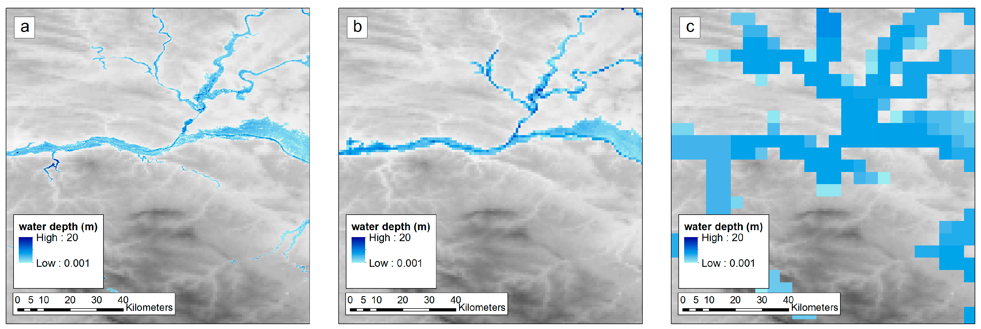
  • ISIMIP average impacts are the largest in most countries (31 countries out of 38), which can be attributed to the methodology that considers the whole river network irrespective of the upstream area of catchments. In addition, the coarser resolution of flood maps produces larger flood extents, and in turn, impacts (see Figure 1). JRC-EU average impacts are the largest in 6 out of 38 countries, including Czech Republic, Croatia, Ireland, Luxembourg, Poland, and Slovenia, while JRC-GL average impacts are the largest only in Latvia, though with a similar value to the other two ensemble means.
  • JRC-GL baseline impacts are the smallest of the three in most countries, due to the reduced extent of the river network considered (i.e., only rivers with upstream area above 5000 km2). Indeed, results from the JRC-GL and consequent projected changes under global warming could be considered as representative of the flood risk in large rivers only.
  • In most countries, the confidence bands of the ensembles intersect the range of reported economic losses. However, ISIMIP results for some countries are well above this range, notably for Ukraine and Italy. This is in line with the results of the evaluation exercise performed by Dottori et al. [21] for ISIMIP, who observed an overestimation of impacts for some European countries. To provide a measure of the accuracy currently attainable with state-of-the-art flood damage models, recent works showed that the expected difference between simulations and observations can be of a factor of two or even more [54].
  • Uncertainties and limitations in the available impact datasets are a known issue [55], especially for global datasets [56], though this issue can be partly addressed through the use of simulated impacts [57]. Main issues include under-reporting of minor flood events and of those further back in time, absence of economic loss data for a large part of reported events, and uneven data coverage across European countries (e.g., fewer data for Eastern European countries before 1990 and in particular for countries that were part of the Soviet Union). For example, a comparison of national disaster loss databases with EM-DAT data showed that total losses can be up to 60% higher when data from high-frequency, low-severity events are accounted for [29].
Results in terms of affected population are comparable to those of economic damages, with similar spread in the ensemble results, though with a clear tendency of model results to be higher than reported figures (Figure 3). For population, it must be noted that observed data come only from the EM-DAT database and that the evaluation of population affected is more complex and prone to errors due to different standards for reporting the number of people hit by floods [58].
Figure 4 summarizes the agreement between the three ensemble averages for each country and SWL scenario, considering the sign of projected changes in flood impact. The agreement is evaluated giving the same weight to each ensemble and using +/− signs as follows:
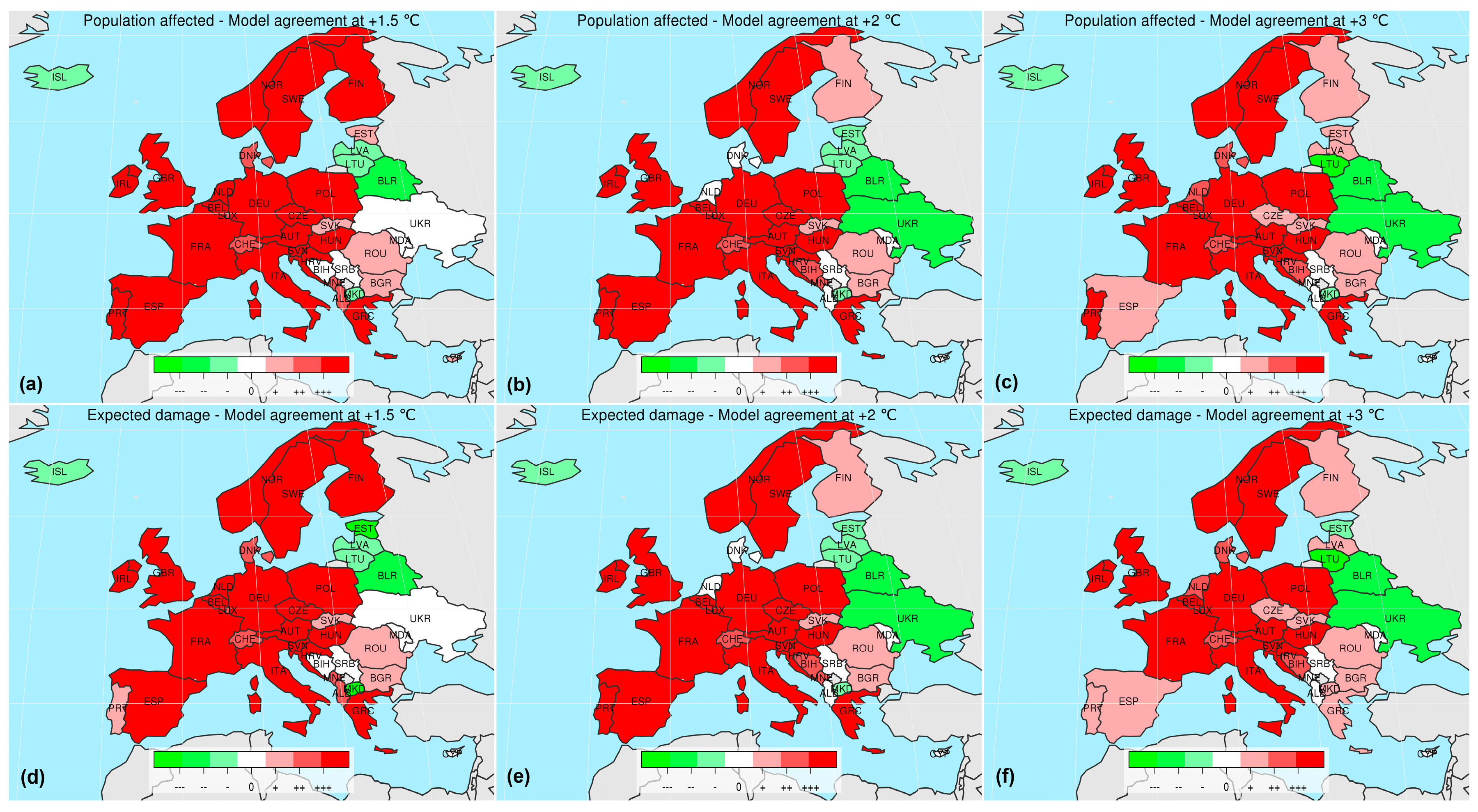
  • +++ (−−−) : all cases predict an increase (decrease) in impacts;
  • ++ (−−) : two cases predict an increase (decrease) in impacts, results are not available for the third (see Section 2.2.1);
  • + (−) : this is used for two cases: (1) two cases predict an increase (decrease) in impacts while a third predicts an opposite change; or (2) only one case study is available and predicts an increase (decrease) in impacts;
  • 0: only two ensembles available and predicting opposite changes in impacts.
The spatial distribution of the model agreement shows that the three flood risk assessments agree on an increasing trend in most of Western and Central European countries, and on a decreasing trend in Eastern countries. Model results are more variable in a number of northern countries like Iceland, Finland, Estonia, and Latvia, and in most south-eastern countries, with the exception of Greece. Interestingly, impact trends for the British Isles and for Eastern Europe mostly agree with those identified by Kundzewicz et al. [19].
Figure 5 and Figure 6 focus on the future impacts predicted by the model ensembles, showing the relative change for each SWL and country with respect to the baseline. The plots allow comparisons of the magnitude of predicted changes, complementing the information shown in Figure 2 and Figure 3 with a quantitative assessment. Some considerations can be drawn from those figures:
  • In most countries in Western and Central Europe, all models consistently predict a relevant increase in future flood impacts.
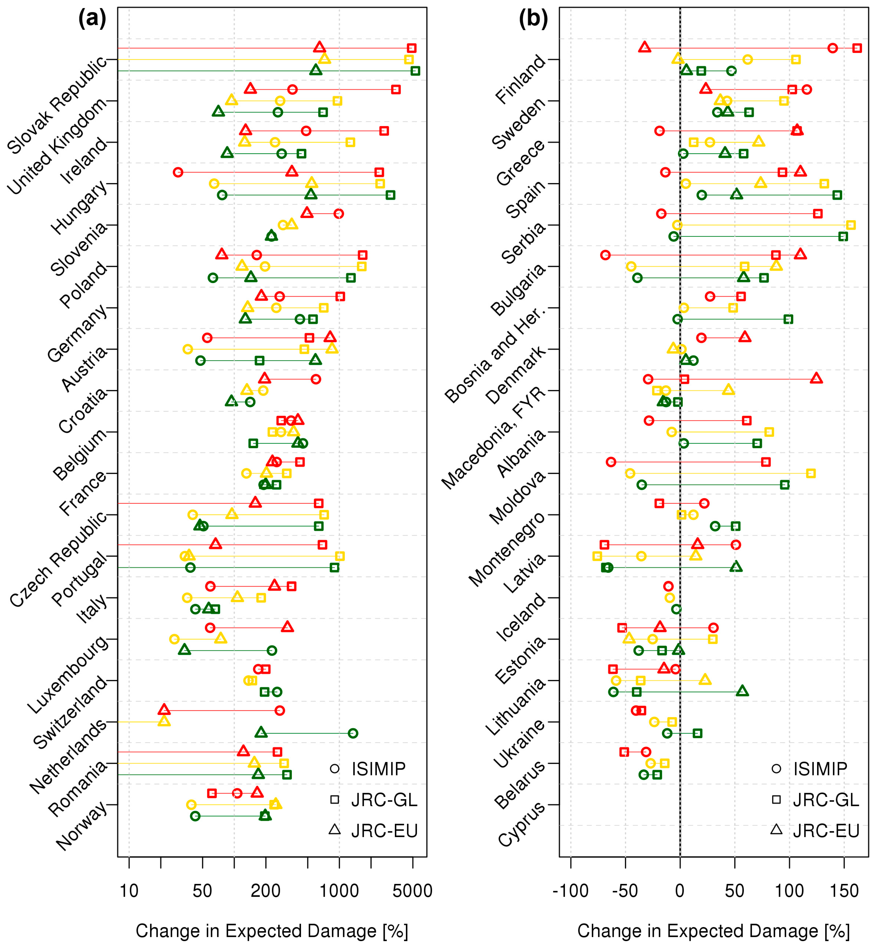
  • The largest changes are usually predicted by the JRC-GL, which projects a more than 10-fold increase in impacts in the Slovak Republic, Hungary, and Poland. Conversely, the ISIMIP ensemble predicts smaller changes, with JRC-EU generally in between. In particular, ISIMIP predicts a negative change for several south-eastern and eastern countries, while JRC-EU and JRC-GL foresee a decrease only in few countries.
  • For the vast majority of countries, projected changes in flood risk for each of the three models along the SWLs differ considerably less than the corresponding changes among models, for each specific SWL. Country average range of percent change in flood risk along SWLs is of 180% for expected damages and 170% for population affected. Such values are smaller in comparison to the average range of percent change in flood risk along the three models, which is of 490% for expected damages and 540% for population affected.
  • The trend of flood risk for increasing warming levels is similar for the three models, for most countries. However, notable exceptions are found in Poland, Germany, Czech Republic, Finland, Sweden, Spain, and Bulgaria, where at least two out of the three models show a monotonic trend of the opposite sign (e.g., in Poland, expected damage estimates from JRC-EU decrease with higher warming levels, while estimates from JRC-GL increase with the SWLs).
  • In a number of countries, impacts may largely increase even in the case of limiting future warming to 1.5 °C.
Further insight on the spread of relative changes at country level for each ensemble and each SWL is given in Supplement Figures S1–S6. Those figures show the large variability in impact estimates of specific ensemble members, which stresses the challenge in characterizing the overall uncertainty of the three combined ensemble estimates.
Summary impact projections and relative changes from the baseline for the three cases are shown in Table 2 for expected damage and Table 3 for population affected. The JRC-EU provides the best estimates of flood impacts at the European level for the baseline period, where reported annual figures are between 4.3 and 8 B€ (5 B€ for JRC-EU) of losses and 262,000 (216,000 for JRC-EU) people affected by flood events in Europe [59,60]. Average relative changes in flood impacts of the three ensembles (super-ensemble) rise with the SWLs from 113% (expected damage) and 86% (population affected) at 1.5 °C, up to 145% and 123%, respectively, at 3 °C. These are the result of averaging a marked increase in flood risk by the JRC-EU and JRC-GL, with the ISIMIP predictions which point to an initial growth of impacts at 1.5 °C and then a further stabilization for higher SWLs. One should note that JRC-EU and JRC-GL are more likely to identify non-linear trends in flood risk, thanks to the POT approach that enables the detection of non-linear changes in the frequency of future floods. Similarly, the coarser resolution inundation model of ISIMIP, coupled with flooded fraction maps, is prone to underestimating non-linear changes in the flood impacts.

4. Discussion and Conclusions

This work presents, for the first time to our knowledge, a quantitative comparison of socio-economic impact projections of river floods in Europe under climate change, derived by three research works based on state-of-the-art models and datasets. We included only those three case studies in the comparison, due to the very limited availability of large scale assessments of the future impacts of natural hazards under specific warming levels. Nation-wide risk assessments have the advantage of: (1) enabling the comparison of methods set up at different spatial grid resolutions; and (2) enabling the comparison of modeled impact estimates over a set of past years with reported aggregated values available from disaster losses datasets.
As expected, the quantitative comparison of results shows significant differences among the three assessments, which may depend on different modelling components and data used in each case study. Part of these differences can be attributed to the use of different climate and hydrological models. While the uncertainty related to the climatological forcing is well known in the literature, results from Dottori et al. [21] show that the hydrological modeling component may also have a significant impact. The resolution of flood maps and of the driving inundation models also play a prominent role in determining the overall impact estimates. In this regard, we stress the importance of using high resolution inundation modeling to achieve accurate impact estimates. This is presently limited by the scarce availability of high resolution Digital Elevation Models (DEM) over large areas, where small scale features are able to influence considerably the distribution of the floodwaters. Results from the three ensemble projections and their distributions suggest that multi-ensemble averaging can be one way to improve the robustness of impact estimates. However, a rigorous characterization of the multi-model uncertainty appears a more challenging task, due to the strong heterogeneity between the distributions of the three ensemble projections. Moreover, expert knowledge on specific modeling components and their limitations can help in identifying more realistic ranges of uncertainty. Approaches based on Bayesian statistics are a possible way forward to account for such prior information and improve the predictive uncertainty, provided that these are quantified within realistic ranges.
Regarding impact modelling, the three cases here considered use similar approaches, mainly based on the simulated extent and depth of flooding. There is a wide variety of flood damage models in use that can differ substantially in methodological aspects and economic estimates. The datasets and resolution of exposure data may be an additional factor in explaining differences in results, as shown by a comparative quantitative flood damage model assessment by Jongman et al. [61].
Overall, we found JRC-EU to produce the best quantitative estimates of past impacts as compared to the other two cases, most likely due to the higher resolution and better quality of the underlying models and datasets. Nevertheless, we found that all the three cases produced results comparable with observed loss data. This is an important result because the performance for present-day conditions does not necessarily imply skillful prediction of future changes, and therefore, the joint analysis of multiple case studies can help identify more robust trends in the future flood risk in Europe.
Results from the three assessments suggest that climate projections are the main driver influencing future trends of flood risk under global warming. Moreover, the uncertainty attributed to the climate projections is likely to be underestimated due to the relatively small, though widely used, model ensembles [62]. Other factors such as the bias correction of climate projections, the method for assessing the year of exceeding SWLs, and the spatial resolution of the input data, surely do influence results though probably to a smaller degree, and do not affect the direction of the projected changes. Despite some differences in the absolute and relative change in projected flood impacts at SWLs, the three cases showed a generally good agreement in the spatial distribution of the direction of changes. In detail, most of the Central and Western Europe is consistently projected to experience substantial increase in flood risk at all SWLs, with the magnitude of the change increasing for higher levels of warming. Conversely, some persistence in the signal of decrease in flood risk with warmer temperatures is found in some countries in Eastern Europe, though in most occasions the three case studies provided contrasting results, showing that highest uncertainties are located in Eastern Europe and particularly in the Balkan region. Interestingly, in some countries in Southern Europe (Spain, Portugal, Greece), the initial increase in impacts at 1.5 °C turns into more uncertain projections in the case of higher warming levels, due to a consequent substantial reduction in the mean annual precipitation.
Future works should focus on quantifying the influence of specific modelling components or datasets by systematically comparing different versions of the same modelling framework. While similar studies would be demanding, given the amount of data and computational times required to run a full flood impact modelling chain, we believe that more similar case studies should be carried out to improve the robustness and reliability of flood risk estimates. To this end, the evaluation of flood impact models within inter-comparison projects such as ISIMIP is a valid option to progress further.
This work confirms that the impacts of global warming on river flood risk in Europe are widespread and often significant, though they can vary in sign and magnitude from region to region. The Paris Agreement has set critical thresholds of warming that we must aim for, yet it has demanded that the scientific community provide additional evidence on the possible effects of warming on the consequent impacts on the society. Our results show that substantial impacts can be avoided by limiting global warming to lower temperature thresholds. However, a considerable increase in flood risk is predicted in Europe even under the most optimistic scenario of 1.5 °C warming as compared to pre-industrial levels, urging national governments to prepare effective adaptation plans to compensate for the foreseen increasing risks.

Supplementary Materials

The following are available online at https://www.mdpi.com/2225-1154/6/1/6/s1.
Supplementary File 1

Acknowledgments

The research leading to these results has received funding from the European Union Seventh Framework Programme FP7/2007–2013 under grant agreement no 603864 (HELIX: “High-End cLimate Impacts and eXtremes”; www.helixclimate.eu).

Author Contributions

Lorenzo Alfieri, Francesco Dottori and Luc Feyen conceived and designed the experiments; Lorenzo Alfieri and Francesco Dottori performed the experiments and analyzed the data. All authors contributed to writing the paper.

Conflicts of Interest

The authors declare no conflict of interest.

References

  1. European Environment Agency (EEA). Economic Losses from Climate-Related Extremes; European Environment Agency (EEA): Copenhagen, Denmark, 2017; p. 17. [Google Scholar]
  2. Forzieri, G.; Feyen, L.; Russo, S.; Vousdoukas, M.; Alfieri, L.; Outten, S.; Migliavacca, M.; Bianchi, A.; Rojas, R.; Cid, A. Multi-hazard assessment in Europe under climate change. Clim. Chang. 2016, 1–15. [Google Scholar] [CrossRef]
  3. IPCC. Managing the Risks of Extreme Events and Disasters to Advance Climate Change Adaptation. A Special Report of Working Groups I and II of the Intergovernmental Panel on Climate Change; Field, C.B., Barros, V., Stocker, T.F., Qin, D., Dokken, D.J., Ebi, K.L., Mastrandrea, M.D., Mach, K.J., Plattner, G.-K., Allen, S.K., Eds.; Cambridge University Press: Cambridge, UK; New York, NY, USA, 2012. [Google Scholar]
  4. Falter, D.; Schröter, K.; Dung, N.V.; Vorogushyn, S.; Kreibich, H.; Hundecha, Y.; Apel, H.; Merz, B. Spatially coherent flood risk assessment based on long-term continuous simulation with a coupled model chain. J. Hydrol. 2015, 524, 182–193. [Google Scholar] [CrossRef]
  5. Morita, M. Quantification of increased flood risk due to global climate change for urban river management planning. Water Sci. Technol. 2011, 63, 2967–2974. [Google Scholar] [CrossRef] [PubMed]
  6. Foudi, S.; Osés-Eraso, N.; Tamayo, I. Integrated spatial flood risk assessment: The case of Zaragoza. Land Use Policy 2015, 42, 278–292. [Google Scholar] [CrossRef]
  7. Rojas, R.; Feyen, L.; Watkiss, P. Climate change and river floods in the European Union: Socio-economic consequences and the costs and benefits of adaptation. Glob. Environ. Chang. 2013, 23, 1737–1751. [Google Scholar] [CrossRef]
  8. Winsemius, H.C.; Van Beek, L.P.H.; Jongman, B.; Ward, P.J.; Bouwman, A. A framework for global river flood risk assessments. Hydrol. Earth Syst. Sci. 2013, 17, 1871–1892. [Google Scholar] [CrossRef] [Green Version]
  9. Ward, P.J.; Jongman, B.; Aerts, J.C.J.H.; Bates, P.D.; Botzen, W.J.W.; Diaz Loaiza, A.; Hallegatte, S.; Kind, J.M.; Kwadijk, J.; Scussolini, P.; et al. A global framework for future costs and benefits of river-flood protection in urban areas. Nat. Clim. Chang. 2017. [Google Scholar] [CrossRef]
  10. Arnell, N.W.; Gosling, S.N. The impacts of climate change on river flood risk at the global scale. Clim. Chang. 2014, 1–15. [Google Scholar] [CrossRef]
  11. Jiménez, C.; Oki, T.; Arnell, N.W.; Benito, G.; Cogley, J.G.; Döll, P.; Jiang, T.; Mwakalila, S.S.; Kundzewicz, Z.; Nishijima, A. Freshwater resources. In Climate Change 2014 Impacts, Adaptation and Vulnerability: Part A: Global and Sectoral Aspects; Intergovernmental Panel on Climate Change (IPCC): Geneva, Switzerland, 2015; pp. 229–270. [Google Scholar]
  12. Taylor, K.E.; Stouffer, R.J.; Meehl, G.A. An Overview of CMIP5 and the Experiment Design. Bull. Am. Meteorol. Soc. 2012, 93, 485–498. [Google Scholar] [CrossRef]
  13. Dankers, R.; Arnell, N.W.; Clark, D.B.; Falloon, P.D.; Fekete, B.M.; Gosling, S.N.; Heinke, J.; Kim, H.; Masaki, Y.; Satoh, Y.; et al. First look at changes in flood hazard in the Inter-Sectoral Impact Model Intercomparison Project ensemble. Proc. Natl. Acad. Sci. USA 2014, 111, 3257–3261. [Google Scholar] [CrossRef] [PubMed]
  14. Jacob, D.; Petersen, J.; Eggert, B.; Alias, A.; Christensen, O.B.; Bouwer, L.M.; Braun, A.; Colette, A.; Déqué, M.; Georgievski, G.; et al. EURO-CORDEX: New high-resolution climate change projections for European impact research. Reg. Environ. Chang. 2014, 14, 563–578. [Google Scholar] [CrossRef]
  15. McSweeney, C.F.; Jones, R.G.; Booth, B.B.B. Selecting Ensemble Members to Provide Regional Climate Change Information. J. Clim. 2012, 25, 7100–7121. [Google Scholar] [CrossRef]
  16. Schleussner, C.-F.; Lissner, T.K.; Fischer, E.M.; Wohland, J.; Perrette, M.; Golly, A.; Rogelj, J.; Childers, K.; Schewe, J.; Frieler, K.; et al. Differential climate impacts for policy-relevant limits to global warming: The case of 1.5 °C and 2 °C. Earth Syst. Dyn. 2016, 7, 327–351. [Google Scholar] [CrossRef] [Green Version]
  17. Field, C.B.; Barros, V.R.; Mach, K.; Mastrandrea, M. Part 2 of Climate Change 2014: Impacts, Adaptation, and Vulnerability: Working Group II Contribution to the Fifth Assessment Report of the Intergovernmental Panel on Climate Change; Cambridge University Press: Cambridge, UK, 2014; pp. 1–76. [Google Scholar]
  18. Kundzewicz, Z.W.; Lugeri, N.; Dankers, R.; Hirabayashi, Y.; Döll, P.; Pińskwar, I.; Dysarz, T.; Hochrainer, S.; Matczak, P. Assessing river flood risk and adaptation in Europe—Review of projections for the future. Mitig. Adapt. Strateg. Glob. Chang. 2010, 15, 641–656. [Google Scholar] [CrossRef]
  19. Kundzewicz, Z.W.; Pińskwar, I.; Brakenridge, G.R. Changes in river flood hazard in Europe: A review. Hydrol. Res. 2017. [Google Scholar] [CrossRef]
  20. Alfieri, L.; Feyen, L.; Dottori, F.; Bianchi, A. Ensemble flood risk assessment in Europe under high end climate scenarios. Glob. Environ. Chang. 2015, 35, 199–212. [Google Scholar] [CrossRef]
  21. Dottori, F.; Szewczyk, W.; Ciscar, J.C.; Zhao, F.; Alfieri, L.; Hirabayashi, Y.; Bianchi, A.; Frieler, K.; Betts, R.A.; Feyen, L. Global human and economic losses from river floods under the Paris climate mitigation targets. Nat. Clim. Chang. 2018. in review. [Google Scholar]
  22. Alfieri, L.; Bisselink, B.; Dottori, F.; Naumann, G.; de Roo, A.; Salamon, P.; Wyser, K.; Feyen, L. Global projections of river flood risk in a warmer world. Earths Future 2017, 5, 171–182. [Google Scholar] [CrossRef]
  23. United Nations Framework Convention on Climate Change (UNFCCC). Paris Agreement, Conference of the Parties, Twenty-First Session (COP21); United Nations Framework Convention on Climate Change: Paris, France, 2015. [Google Scholar]
  24. Jongman, B.; Hochrainer-Stigler, S.; Feyen, L.; Aerts, J.C.J.H.; Mechler, R.; Botzen, W.J.W.; Bouwer, L.M.; Pflug, G.; Rojas, R.; Ward, P.J. Increasing stress on disaster-risk finance due to large floods. Nat. Clim. Chang. 2014, 4, 264–268. [Google Scholar] [CrossRef]
  25. Donnelly, C.; Greuell, W.; Andersson, J.; Gerten, D.; Pisacane, G.; Roudier, P.; Ludwig, F. Impacts of climate change on European hydrology at 1.5, 2 and 3 degrees mean global warming above preindustrial level. Clim. Chang. 2017, 143, 13–26. [Google Scholar] [CrossRef]
  26. Thober, S.; Kumar, R.; Wanders, N.; Marx, A.; Pan, M.; Rakovec, O.; Samaniego, L.; Sheffield, J.; Wood, E.F.; Zink, M. Multi-model ensemble projections of European river floods and high flows at 1.5, 2, and 3 degrees global warming. Environ. Res. Lett. 2018, 13, 014003. [Google Scholar] [CrossRef]
  27. EM-DAT. The OFDA/CRED International Disaster Database; Université Catholique de Louvain: Brussels, Belgium, 2016; Available online: www.emdat.be (accessed on 16 January 2018).
  28. Munich Re. NatCatSERVICE—Loss Events Worldwide 1980–2014; Munich Re: Munich, Germany, 2015; p. 10. [Google Scholar]
  29. United Nations Office for Disaster Risk Reduction (UNISDR). Making Development Sustainable, the Future of Disaster Risk Management: Global Assessment Report on Disaster Risk Reduction 2015; United Nations Office for Disaster Risk Reduction (UNISDR): Geneva, Switzerland, 2015; p. 316. [Google Scholar]
  30. Van der Knijff, J.M.; Younis, J.; de Roo, A.P.J. LISFLOOD: A GIS-based distributed model for river basin scale water balance and flood simulation. Int. J. Geogr. Inf. Sci. 2010, 24, 189–212. [Google Scholar] [CrossRef]
  31. Burek, P.; van der Knijff, J.; de Roo, A. LISFLOOD, Distributed Water Balance and Flood Simulation Model Revised User Manual 2013; Publications Office: Luxembourg, 2013; ISBN 978-92-79-33191-6. [Google Scholar]
  32. Alfieri, L.; Salamon, P.; Bianchi, A.; Neal, J.; Bates, P.; Feyen, L. Advances in pan-European flood hazard mapping. Hydrol. Process. 2014, 28, 4067–4077. [Google Scholar] [CrossRef]
  33. Yamazaki, D.; Kanae, S.; Kim, H.; Oki, T. A physically based description of floodplain inundation dynamics in a global river routing model. Water Resour. Res. 2011, 47, W04501. [Google Scholar] [CrossRef]
  34. Pesaresi, M.; Huadong, G.; Blaes, X.; Ehrlich, D.; Ferri, S.; Gueguen, L.; Halkia, M.; Kauffmann, M.; Kemper, T.; Lu, L.; et al. A global human settlement layer from optical HR/VHR RS data: Concept and first results. IEEE J. Sel. Top. Appl. Earth Obs. Remote Sens. 2013, 6, 2102–2131. [Google Scholar] [CrossRef]
  35. Bontemps, S.; Defourny, P.; Bogaert, E.V.; Arino, O.; Kalogirou, V.; Perez, J.R. GLOBCOVER 2009—Products Description and Validation Report; Universite’ catholique de Louvain (UCL) and European Space Agency (ESA): Louvain, Belgium, 2011. [Google Scholar]
  36. Scussolini, P.; Aerts, J.C.J.H.; Jongman, B.; Bouwer, L.M.; Winsemius, H.C.; de Moel, H.; Ward, P.J. FLOPROS: An evolving global database of flood protection standards. Nat. Hazards Earth Syst. Sci. 2016, 16, 1049–1061. [Google Scholar] [CrossRef]
  37. Huizinga, H.J.; De Moel, H. Global Flood Damage Functions—Report Tasks 1&2: Review of Existing Data Sources and Global Flood Damage Functions Database; HKV Lijn in Water: Lelystad, The Netherlands, 2016. [Google Scholar]
  38. Hazeleger, W.; Wang, X.; Severijns, C.; Ştefǎnescu, S.; Bintanja, R.; Sterl, A.; Wyser, K.; Semmler, T.; Yang, S.; van den Hurk, B.; et al. EC-Earth V2.2: Description and validation of a new seamless earth system prediction model. Clim. Dyn. 2012, 39, 2611–2629. [Google Scholar] [CrossRef]
  39. Dottori, F.; Todini, E. Developments of a flood inundation model based on the cellular automata approach: Testing different methods to improve model performance. Phys. Chem. Earth Parts ABC 2011, 36, 266–280. [Google Scholar] [CrossRef]
  40. Bates, P.D.; Horritt, M.S.; Fewtrell, T.J. A simple inertial formulation of the shallow water equations for efficient two-dimensional flood inundation modelling. J. Hydrol. 2010, 387, 33–45. [Google Scholar] [CrossRef]
  41. Batista e Silva, F.; Gallego, J.; Lavalle, C. A high-resolution population grid map for Europe. J. Maps 2013, 9, 16–28. [Google Scholar] [CrossRef]
  42. Batista e Silva, F.; Lavalle, C.; Koomen, E. A procedure to obtain a refined European land use/cover map. J. Land Use Sci. 2013, 8, 255–283. [Google Scholar] [CrossRef]
  43. Huizinga, H.J. Flood Damage Functions for EU Member States; HKV Lijn in Water: Lelystad, The Netherlands, 2007; p. 67. [Google Scholar]
  44. Hempel, S.; Frieler, K.; Warszawski, L.; Schewe, J.; Piontek, F. A trend-preserving bias correction—The ISI-MIP approach. Earth Syst. Dyn. 2013, 4, 219–236. [Google Scholar] [CrossRef]
  45. Betts, R.A.; Alfieri, L.; Caesar, J.; Chang, J.; Ciais, P.; Feyen, L.; Friedlingstein, P.; Gohar, L.; Koutroulis, A.; Papadimitriou, L.V.; et al. Projecting climate extremes, hydrology and vegetation at 1.5 °C and 2 °C global warming with higher-resolution models. Philos. Trans. A 2018. in review. [Google Scholar]
  46. Pendergrass, A.G.; Lehner, F.; Sanderson, B.M.; Xu, Y. Does extreme precipitation intensity depend on the emissions scenario? Geophys. Res. Lett. 2015, 42. [Google Scholar] [CrossRef]
  47. Sangati, M.; Borga, M. Influence of rainfall spatial resolution on flash flood modelling. Nat. Hazards Earth Syst. Sci. 2009, 9, 575–584. [Google Scholar] [CrossRef]
  48. Alfieri, L.; Burek, P.; Feyen, L.; Forzieri, G. Global warming increases the frequency of river floods in Europe. Hydrol. Earth Syst. Sci. 2015, 19, 2247–2260. [Google Scholar] [CrossRef] [Green Version]
  49. Dottori, F.; Salamon, P.; Bianchi, A.; Alfieri, L.; Hirpa, F.A.; Feyen, L. Development and evaluation of a framework for global flood hazard mapping. Adv. Water Resour. 2016, 94, 87–102. [Google Scholar] [CrossRef]
  50. Ntegeka, V.; Salamon, P.; Gomes, G.; Sint, H.; Lorini, V.; Thielen, J.; Zambrano-Bigiarini, M. EFAS-Meteo: A European Daily High-Resolution Gridded Meteorological Data Set for 1990–2011; Publications Office of the European Union: Luxembourg, 2013. [Google Scholar]
  51. Dee, D.P.; Uppala, S.M.; Simmons, A.J.; Berrisford, P.; Poli, P.; Kobayashi, S.; Andrae, U.; Balmaseda, M.A.; Balsamo, G.; Bauer, P.; et al. The ERA-Interim reanalysis: Configuration and performance of the data assimilation system. Q. J. R. Meteorol. Soc. 2011, 137, 553–597. [Google Scholar] [CrossRef]
  52. Blöschl, G.; Ardoin-Bardin, S.; Bonell, M.; Dorninger, M.; Goodrich, D.; Gutknecht, D.; Matamoros, D.; Merz, B.; Shand, P.; Szolgay, J. At what scales do climate variability and land cover change impact on flooding and low flows? Hydrol. Process. 2007, 21, 1241–1247. [Google Scholar] [CrossRef]
  53. Apollonio, C.; Balacco, G.; Novelli, A.; Tarantino, E.; Piccinni, A.F. Land Use Change Impact on Flooding Areas: The Case Study of Cervaro Basin (Italy). Sustainability 2016, 8, 996. [Google Scholar] [CrossRef]
  54. Wagenaar, D.J.; de Bruijn, K.M.; Bouwer, L.M.; de Moel, H. Uncertainty in flood damage estimates and its potential effect on investment decisions. Nat. Hazards Earth Syst. Sci. 2016, 16, 1–14. [Google Scholar] [CrossRef]
  55. Thieken, A.H.; Bessel, T.; Kienzler, S.; Kreibich, H.; Müller, M.; Pisi, S.; Schröter, K. The flood of June 2013 in Germany: How much do we know about its impacts? Nat. Hazards Earth Syst. Sci. 2016, 16, 1519–1540. [Google Scholar] [CrossRef]
  56. Huggel, C.; Raissig, A.; Rohrer, M.; Romero, G.; Diaz, A.; Salzmann, N. How useful and reliable are disaster databases in the context of climate and global change? A comparative case study analysis in Peru. Nat. Hazards Earth Syst. Sci. 2015, 15, 475–485. [Google Scholar] [CrossRef] [Green Version]
  57. Alfieri, L.; Feyen, L.; Salamon, P.; Thielen, J.; Bianchi, A.; Dottori, F.; Burek, P. Modelling the socio-economic impact of river floods in Europe. Nat. Hazards Earth Syst. Sci. 2016, 16, 1401–1411. [Google Scholar] [CrossRef] [Green Version]
  58. Guha-Sapir, D.; Vos, F.; Below, R.; Ponserre, S. Annual Disaster Statistical Review 2011: The Numbers and Trends; CRED: Brussels, Belgium, 2012. [Google Scholar]
  59. Association of British Insurers (ABI). Financial Risks of Climate Change—Summary Report; Association of British Insurers: London, UK, 2005. [Google Scholar]
  60. European Environment Agency (EEA). Mapping the Impacts of Natural Hazards and Technological Accidents in Europe—An Overview of the Last Decade; European Environment Agency: Copenhagen, Denmark, 2010; p. 144. [Google Scholar]
  61. Jongman, B.; Kreibich, H.; Apel, H.; Barredo, J.I.; Bates, P.D.; Feyen, L.; Gericke, A.; Neal, J.; Aerts, J.C.J.H.; Ward, P.J. Comparative flood damage model assessment: Towards a European approach. Nat. Hazards Earth Syst. Sci. 2012, 12, 3733–3752. [Google Scholar] [CrossRef] [Green Version]
  62. McSweeney, C.F.; Jones, R.G. How representative is the spread of climate projections from the 5 CMIP5 GCMs used in ISI-MIP? Clim. Serv. 2016, 1, 24–29. [Google Scholar] [CrossRef]
Figure 1. Inundation maps for a 1-in-100-year flood event from the three cases for Central France, with resolution between parentheses. (a) JRC Europe (JRC-EU) (100 m); (b) JRC Global (JRC-GL) (~1 km); (c) Inter-Sectorial Impacts Model Intercomparison Project (ISIMIP) (~5 km). Note that for each flooded cell of the ISIMIP grid, the fraction of area inundated is also given.
Climate 06 00006 g001
Figure 2. Economic damage computed for the baseline period for each country by the ensembles of the three case studies (a,b). Plots show the average (black dash), ±1 standard deviation (colored bar), and minimum and maximum values (whiskers) of each ensemble. The gold bars show the range of reported impact values (minimum and maximum).
Climate 06 00006 g002
Figure 3. Population affected computed for the baseline period for each country by the ensembles of the three case studies (a,b). Plots show the average (black dash), ±1 standard deviation (colored bar), and minimum and maximum values (whiskers) of each ensemble. In gold are shown impact values reported in the Emergency Events Database (EM-DAT).
Climate 06 00006 g003
Figure 4. Multi-model agreement of projected changes in affected population (ac) and expected damage (df) at specific warming levels (SWLs): 1.5 °C (a,d), 2 °C (b,e), and 3 °C (c,f). Colors depend on the number of cases predicting a positive or negative change in impacts.
Climate 06 00006 g004
Figure 5. Relative average change in expected damage for 1.5 °C (green), 2 °C (yellow), and 3 °C (red) warming scenarios with respect to the baseline, calculated at country level for the three ensembles (a,b). Note that the x-axis in (a) uses a logarithmic scale.
Climate 06 00006 g005
Figure 6. Relative average change in population affected for 1.5 °C (green), 2 °C (yellow), and 3 °C (red) warming scenarios with respect to the baseline, calculated at country level for the three ensembles (a,b). Note that the x-axis in (a) uses a logarithmic scale.
Climate 06 00006 g006
Table 1. Modeling components included in the three flood risk assessment studies and relevant references.
Authors (Application)GCMRCMHydrological ModelFlood EventsInundation Model (Resolution)Exposure DataVulnerability Data
Dottori et al. [21] (ISIMIP)GFDL-ESM2M *
HadGEM2-ES *
IPSL-CM5A-LR *
MIROC-ESM-CHEM *
NorESM1-M *
-DBH
H08
Mac-PDM.09
MATSIRO
MPI-HM
PCR-GLOBWB
VIC
WBMplus
JULES
LPJmL [13]
Annual maximaCaMa flood [33]
(2.5 arc-min, ~5 km)
GHSL [34]
GlobCover 2009 [35]
FLOPROS [36]
Global damage functions [37]
Alfieri et al. [22] (JRC-GL)IPSL-CM5A-LR
GFDL-ESM2M
HadGEM2-ES
EC-EARTH
GISS-E2-H
IPSL-CM5A-MR
HadCM3LC
EC-EARTH3-HR [38]Lisflood [30]POTCA2D [39] (~1 km)GHSL [34]
GlobCover 2009 [35]
FLOPROS [36]
Global damage functions [37]
Alfieri et al. [20] (JRC-EU)EC-EARTH
HadGEM2-ES
MPI-ESM-LR
RACMO22E
REMO2009
CCLM4-8-17
RCA4 [14]
Lisflood [30]POTLisflood-FP [40]
(100 m)
EU pop [41]
Corine Land Cover [42]
EU flood protections [24]
EU damage functions [43]
* Temperature and precipitation bias corrected according to [44].
Table 2. Expected damage from the three case studies (ensemble average) at specific warming levels (SWLs), including relative change. Averages of the three ensembles are included in the last row.
1.5 °C2 °C3 °C
Expected DamageBaseline (B€/year)Total (B€/year)Relative Change (%)Total (B€/year)Relative Change (%)Total (B€/year)Relative Change (%)
JRC-EU5111161313714173
JRC-GL38188924311331
ISIMIP13269723722697
Super-ensemble7151131511017145
Table 3. Population affected from the three case studies (ensemble average) and at SWLs, including relative change. Averages of the three ensembles are included in the last row.
1.5 °C2 °C3 °C
Population AffectedBaseline (1000 pp/year)Total (1000 pp/year)Relative Change (%)Total (1000 pp/year)Relative Change (%)Total (1000 pp/year)Relative Change (%)
JRC-EU216499131524142600177
JRC-GL156456193509227621299
ISIMIP6799954799146112466
Super-ensemble3506508667493781123

