Regions Subject to Rainfall Oscillation in the 5–10 Year Band


Independent Scholar 1, 96, rue du Port David, 45370 Dry, France
Climate 2018, 6(1), 2; https://doi.org/10.3390/cli6010002
Submission received: 2 December 2017
/
Revised: 28 December 2017
/
Accepted: 3 January 2018
/
Published: 5 January 2018
(This article belongs to the Special Issue Decadal Variability and Predictability of Climate)
Abstract
:The decadal oscillation of rainfall in Europe that has been observed since the end of the 20th century is a phenomenon well known to climatologists. Consequences are considerable because the succession of wet or dry years produces floods or, inversely, droughts. Moreover, much research has tried to answer the question about the possible link between the frequency and the intensity of extra-tropical cyclones, which are particularly devastating, and global warming. This work aims at providing an exhaustive description of the rainfall oscillation in the 5–10 year band during one century on a planetary scale. It is shown that the rainfall oscillation results from baroclinic instabilities over the oceans. For that, a joint analysis of the amplitude and the phase of sea surface temperature anomalies and rainfall anomalies is performed, which discloses the mechanisms leading to the alternation of high and low atmospheric pressure systems. For a prospective purpose, some milestones are suggested on a possible link with very long-period Rossby waves in the oceans.
1. Introduction
The succession of wet and dry periods over decadal cycles that occur in some areas is a well-known phenomenon. Authors paid a particular attention to the quasi-decadal oscillation of rainfall in Europe that has been observed since the end of the 20th century. This phenomenon has been reported in abundant literature [1,2,3], with authors relating studies carried out in Mediterranean areas [4,5], in the Iberian Peninsula [6,7,8,9,10,11,12,13,14], in Italy [15,16], in the UK [17,18], in Ireland [19] and in France [20,21,22].
Rainfall oscillation also occurs in Central-Eastern North America [22,23,24,25,26,27]. Most of the studies rely on the analysis of the North Atlantic Oscillation (NAO). The other regions subject to this alternation are less well documented likely because the rainfall oscillation has occurred during previous decades and is not no longer active presently.
Consequences are considerable because the succession of wet or dry years produces floods or, inversely, droughts, even though the mean precipitation amount is not severely modified [28]. Regions are very differently impacted: some, like Western Europe, Southeastern North America, the region of the Rio de la Plata in South America, Southern Australia or the regions located in the equatorial band between 10° N and 10° S, are heavily impacted, while others like North America north of 50° N, South America between 10° S and 30° S, Asia east of 100° E, Africa between 10° N and 20° S are hardly impacted, excepted a narrow equatorial band. The amplitude of the rainfall oscillation may vary a lot over time, reaching +/−20% of the mean precipitation height during some time intervals or, on the contrary, a few percent the rest of the time.
On the other hand, the formation of subtropical cyclones is another aspect of rainfall oscillation at mid-latitudes. Much research has tried to answer the questions about the possible link between the frequency and the intensity of particularly devastating extra-tropical cyclones and global warming. This work is achieved with the hopes of improving the description of the quasi-decadal oscillation on a planetary scale and proposes plausible explanations. This in view of improving the forecasting of water resources as well as natural disasters.
2. Materials and Methods
2.1. Highlighting Continental Regions Subject to Rainfall Oscillation in the 5–10 Year Band
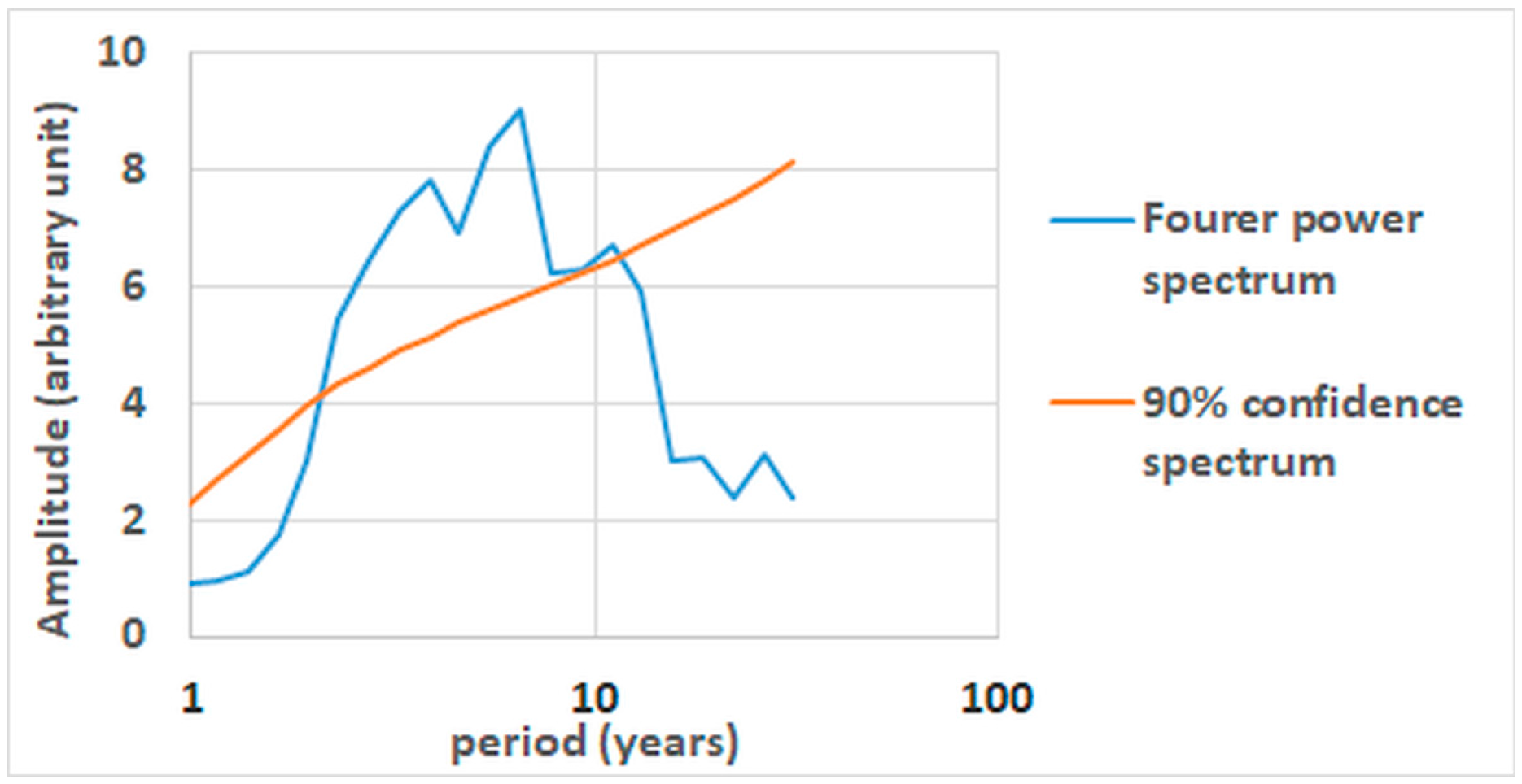
The purpose of the paper is to analyze the rainfall oscillation at mid-latitudes in the 5–10 year band, which proves to be representative of many phenomena both atmospheric and oceanic. If the origin of this oscillation is poorly known, it nevertheless remains that it is ubiquitous, which is reflected, for example, by the Southern Oscillation Index (SOI) (Figure 1). The 5–10 year band is clearly distinct from the characteristic band of the El Niño-Southern Oscillation (ENSO), that is, 1.5–7 years, the latter being centered on the four-year period. The overlapping of these two bands is weak because the absence of any ENSO event during more than five years is rare. The 5–10 year band is mainly representative of phenomena whose cyclicality is of the order of eight years. However, this band must be chosen broad enough because of the large variability of the period of the oscillations.
At mid-latitudes, the oscillation in the 5–10 year band is little dependent on the Pacific Decadal Oscillation (PDO) and the Atlantic Multidecadal Oscillation (AMO) whose Fourier power spectra display a maximum at 5.4 years and 66 years, respectively. Furthermore, the oscillation in the 5–10 year band is distinguished without any ambiguity not only by its frequency, but also by its behavior over time since its amplitude varies a lot, while the PDO and the AMO are more persistent.
The method pursued in this paper consists of jointly analyzing, both in space and time, sea surface temperature (SST) and rainfall oscillations in the 5–10 year band. Wavelet analysis of rainfall and SST series allows representing the regions subject to these oscillation phenomena. For a given rainfall height anomaly, the relevant SST anomaly from which baroclinic instabilities in the atmosphere are responsible for the rainfall oscillation is found thanks to the contrasting behaviors over time of the amplitude of the surrounding SST anomalies. Thus the imprints of the SST and rainfall height anomalies can be unambiguously associated.
Incidentally, wavelet analysis has become a common tool for analyzing localized variations of power within a time series. By decomposing a time series in time-frequency space (actually, time-period space, the period depending on the scale), one is able to determine both the dominant modes of variability and how those modes vary in time. The wavelet transform has been used for numerous studies in geophysics. Pioneer works include tropical convection [29], the ENSO [30,31], atmospheric cold fronts [32], central England temperature [33], the dispersion of ocean waves [34], wave growth and breaking [35], and coherent structures in turbulent flows [36]. More recently, wavelet analysis has been used in the study of rainfall oscillation [11,20,21,22,27].
A Wavelet analysis of rainfall series with a spatial resolution of 0.5 degree allows representing the regions subject to this oscillation phenomenon when the wavelet power is scale-averaged over the 5–10 year band: here, a continuous Morlet wavelet transform is used so that the period and the scale coincide. However, with regard to rainfall series, two precautions must be taken:
- The series must be long enough to represent the rainfall oscillation knowing that its amplitude varies a lot over time, even disappearing during periods of lull.
- Since the average annual rainfall height is not relevant in our analysis, rainfall is reduced, that is, divided by the mean rainfall height. Being dimensionless, the temporal variations of reduced rainfall are homogenized on a global scale: this way the amplitude of the wavelet power only depends on the relative amplitude of the oscillation.
However, the wavelet power is not sufficient when one seeks to correlate different series between them. It is also necessary to specify the phase, which expresses when the oscillation reaches its extrema, with respect to a common temporal reference, which must also display an oscillation in the 5–10 year band. The cross-wavelet analysis of both the reduced rainfall height (RRH) and the temporal reference (TR) expresses the cross-wavelet power and the coherence phase. The cross-wavelet power of RRH and TR divided by the square root of the wavelet power of TR coincides with the square root of the wavelet power of RRH, that is, the amplitude of the RRH oscillation. The coherence phase of RRH and TR shows the time shift between the RRH oscillation and the TR.
Thus, the spatial representation of the oscillations requires paired figures; the first is the amplitude of anomalies (regardless of the time when the anomaly reaches its maximum), and the second is the phase (the time evolution, that is, the time when the anomaly reaches its maximum over a period). The 5–10 year band, over which both the cross-wavelet power and the coherence phase are scale-averaged, allows taking into account the natural broadening of the frequency bands associated with the oscillations.
2.2. The Temporal Reference (TR)
The use of a single temporal reference enables representing the evolution of phenomena on a global scale with a common time base. For phenomena whose periodicity is annual, the temporal reference may be the SST at a very particular place where the intra-annual variability is strong. This choice turns out to be much more difficult for the study of phenomena in the 5–10 year band. A synthetic signal could be used as the temporal reference, for example a sinusoid of eight-year period. However, its zero bandwidth is not suitable. In contrast, the SOI signal is well suited to the problem because it has a broad peak in the 5–10 year band (Figure 1).
Actually, it is not exactly the SOI signal that is used as the TR, but -SOI, that is, the opposite of the SOI signal, this in order to exhibit some homogeneity with the previous publications. If the sign of the TR is not essential in this study, it is not so when it comes to phasing an event in relation to ENSO. In this case, the reference must present a maximum when an ENSO event occurs, so that the sign of the cross-wavelet is not reversed.
2.3. Random Errors
Random data errors, the only ones we are interested in here since both the cross-wavelet power and the coherence phase are unbiased estimators, are easy to evaluate because processing is performed on each pixel independently of the others. Thus, random errors can be estimated from the white noise observed in the spatial representation of phenomena, whether this concerns the amplitude or phase of the oscillations. In practice, the classes are chosen in order to reduce discrepancies between contiguous pixels, so that the amplitude and the phase of the oscillations are represented with an apparent continuity.
2.4. Highlighting SST Anomalies Subject to an Oscillation in the 5–10 Year Band
SST over the oceans can be processed as are the RRH over the continents, from their cross-wavelet power and their coherence phase, by keeping -SOI as the temporal reference (TR) signal. This approach allows comparing the amplitude and the phase of SST and RRH anomalies in space and in time with a common time base, a condition essential for a good understanding of the phenomena observed.
The cross analysis of (SST, -SOI) and (RRH, -SOI) enables observing the coevolution of the amplitude and the phase of SST and RRH anomalies from which causal relationships are drawn. In particular, discerning whether SST and RRH anomalies are in phase or in opposite phase is essential information for decrypting the mechanisms involved in the thermal transfer between oceans and continents, as well as the mechanisms leading to the alternation of high and low atmospheric pressure systems. Because the amplitude of both SST and RRH anomalies may vary considerably over space and time, their comparison versus time allows highlighting the affinity between the two variables without any priori.
2.5. Cross-Wavelet and Complex Empirical Orthogonal Function (EOF) Analyses
A cross-wavelet analysis [22,37] is preferred to a complex EOF analysis to investigate the RRH and SST oscillations within a particular bandwidth. If the two methods are similar for typical frequency domain analyses, that is, the power spectral and coherency analyses, they are far different in terms of the time domain. In complex EOF analysis the time lag between time series is basically the computation of eigenvector and eigenvalue of a covariance or a correlation matrix computed from a group of original time series data. In contrast, the cross-wavelet analysis is well suited to highlight the time lag between time series when it varies continuously.
Applied to SST and RRH data, the cross-wavelet analysis brings out the thermal transfers between oceans and continents as well as their variability from a cycle to another. In particular, by representing the amplitude and the phase of SST and RRH anomalies, the cross-wavelet analysis highlights evaporation above heat sources on the surface of the oceans and the release of latent heat during condensation/precipitation of water vapor above the continents, when they are considered as a unique dynamical phenomenon within a characteristic bandwidth.
2.6. Data
Monthly sea surface temperature (SST) is issued from the Extended Reconstructed Sea Surface Temperatures, version 3 (ERSST.v3), beginning January 1854, provided by the NOAA (National Oceanic and Atmospheric Administration) [38].
Monthly rainfall datasets are month-by-month variation in rainfall height over the last century produced by the Climatic Research Unit (CRU) at the University of East Anglia. They are calculated on high-resolution (0.5 × 0.5 degree) grids, which are based on an archive of monthly mean rainfall height provided by more than 4000 weather stations distributed around the world [39].
The monthly Southern Oscillation Index (SOI), beginning January 1866, is provided by the National Centre for Atmospheric Research [40].
3. Results
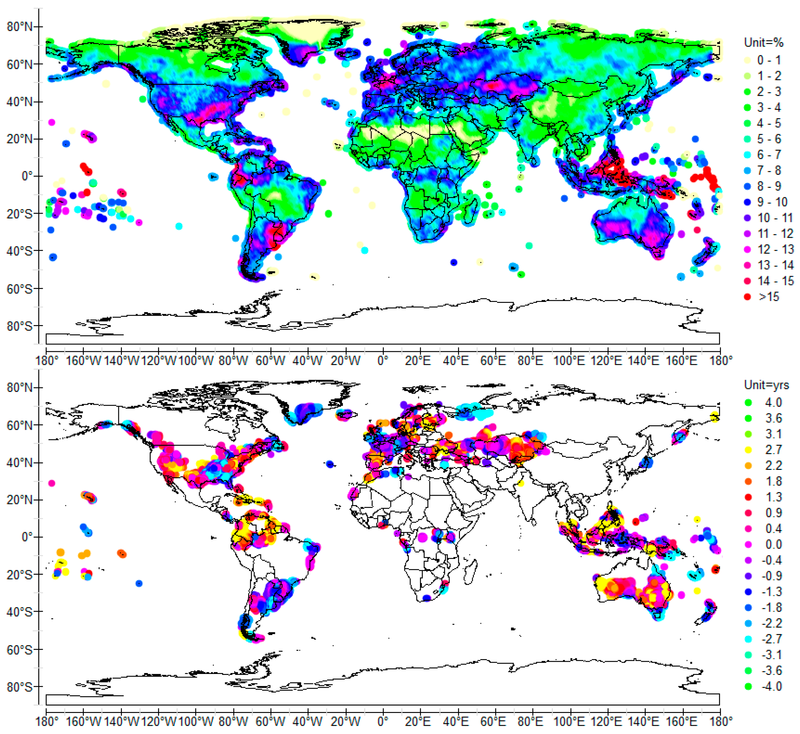
The cross-wavelet power and the coherence phase of RRH, scale-averaged over the 5–10 year band, time-averaged over the entire observation period, allows representing well delimited regions where the rainfall oscillation occurs in the 5–10 year band (Figure 2). The main areas subject to rainfall oscillation at mid-latitudes are: (a) Southwest North America; (b) Texas; (c) Southeastern North America; (d) Northeastern North America; (e) Southern Greenland; (f) Europe and Central and Western Asia; (g) the region of the Río de la Plata; (h) Southwestern and Southeastern Australia, and; (i) Southeast Asia. In contrast, within the tropical belt all continents are subject to the rainfall oscillation in the 5–10 year band.
Amplitude of the RRH oscillation varies between 12% and 15%. The phases where the anomalies reach their maximum are close, except in the south of Australia and in Eastern Europe where it is one or two years late compared to other anomalies. Referring to the work of various authors [41,42,43,44,45,46,47], RRH anomalies could originate from baroclinic instabilities above the oceans all the more so as SST anomalies that occur within this band are ubiquitous as shown below.
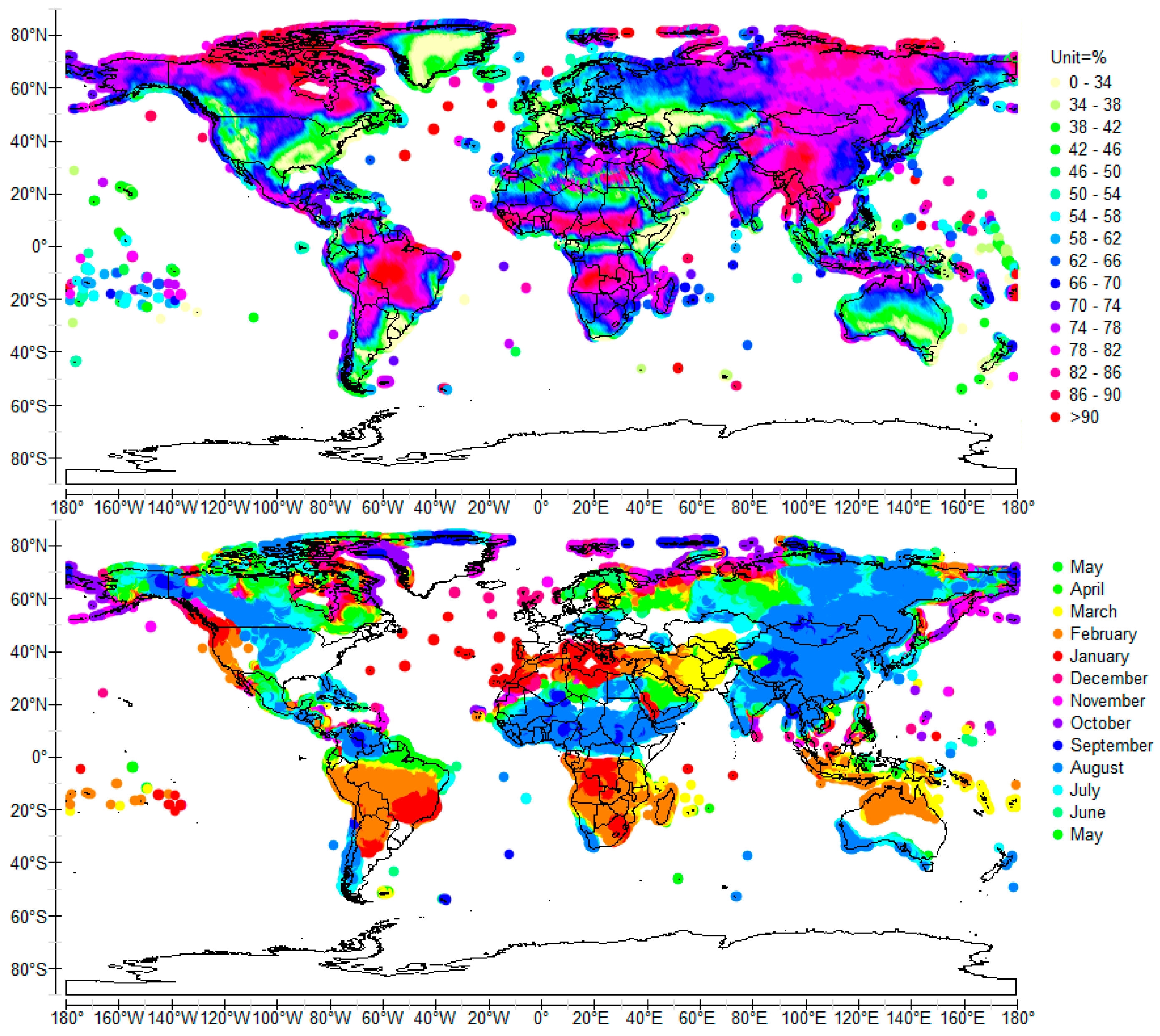
To be convinced of that, it suffices to display the anomalies in the 8–16 month band representative of the annual period (Figure 3). The anomalies in the 5–10 year band correspond to the absence of anomalies in the 8–16 month band. This is true apart from desert regions or those subject to a semi-annual precipitation cycle, which mainly concerns the Horn of Africa and the Greenland Ice Sheet (Figure 4). Outside these regions, the intra-annual variability of RRH is strong, reaching 80–90% of the mean precipitation height. Excluding coastal strips, Mediterranean regions as well as arid and semi-arid regions located in the northern hemisphere (Iran, Iraq and the Persian Gulf states, including Saudi Arabia and Kuwait), the annual rainfall pattern over the continents exhibits a peak time in late summer in both hemispheres, that is, when the difference between the temperature of the air aloft and the surface temperature is the greatest, leading to the greatest potential for instability. The extension of the areas concerned reflects synoptic-scale systems, driven by atmospheric Rossby waves in their respective hemisphere.
On the contrary, rainfall is evenly distributed throughout the year in regions subject to the rainfall oscillation in the 5–10 year band, which discloses the moderating effect of the boundary currents. Annual SST anomalies over subtropical gyres reach their maximum in winter in both hemispheres. Thus, baroclinic low pressure systems occur throughout the year. They are baroclinic since they form along zones of temperature and dew point gradient as will be developed later, taking advantage of the coevolution of both SST and RRH anomalies in the 5–10 year band.
Another consequence of this correspondence between the RRH anomalies in the 5–10 year band and the absence of anomaly in the 8–16 month band is that all regions subject to the 5–10 year band rainfall oscillation are to be considered exhaustively. We will indeed see that the variability over time of the amplitude of anomalies in the 5–10 year band is considerable, but time-averaging the cross-wavelet power over more than one century shows that the rainfall oscillation in that band occurs at least one time a century. It is from these regions that heat exchanges between the oceans and the continents occur primarily, because of latent heat transfer.
3.1. Regions Subject to the RRH Oscillation in the 5–10 Year Band in the Tropics
In the tropics, SST anomalies produce quasi-geostrophic motion of the atmosphere from heating [48]. From the heating zone are formed equatorial-trapped eastward Kelvin waves and westward Rossby waves, hence easterly trade winds set up by atmospheric Kelvin waves to the east and westerlies as an atmospheric planetary wave response to the west. Only a narrow strip is involved in the seesaw of sea level pressure. The impact of the tropical SST anomalies is limited to the equatorial belt between 10° S and 10° N, producing RRH anomalies of average period 1/2, 1, 4 or 8 years through all the continents. The main driver of the RRH oscillation in the tropics is the ENSO.
The most significant rainfall oscillation occurs in Indonesia and in equatorial America where it is closely linked to the SST anomaly extending in the central equatorial Pacific [49]. The RRH anomaly may reach 20% when the SST anomaly in the central Pacific is 0.45 °C (Figure 5). Particularly affected is the strip stretching from Borneo to New Guinea. In contrast, RRH anomaly is lower than 10% when the SST anomaly is low.
RRH anomalies in Indonesia and in equatorial America are out of phase relative to the temporal reference -SOI (Figure 2), while the SST anomaly in the Central Pacific is in phase with -SOI [49]. This is because atmospheric Rossby and Kelvin waves induce high pressure on both sides of the Pacific. A positive SST anomaly induces drought in Indonesia and in equatorial America and, inversely, a negative SST anomaly produces abundant rainfall.
3.2. Regions Subject to the RRH Oscillation in the 5–10 Year Band at Mid-Latitudes
Amplitude of RRH anomalies may vary a lot over time. It vanishes during periods of calm, whereas the alternation of wet and dry episodes has a significant societal impact during the upsurge periods, all the more so as they can produce extreme events leading to floods or droughts.
3.2.1. Rossby Waves in the Oceans at Mid-Latitudes
Long baroclinic Rossby waves play a fundamental role in ocean dynamics and can dramatically affect weather patterns and climate [50]. Because the natural period, that is, the wavelength of Rossby waves at mid-latitudes, adjusts to the forcing period, resonantly forced waves (RFWs) are produced. RFWs enhance modulated geostrophic currents that require an outlet to leave each of the five gyres, merging either with the North Atlantic Drift, or the North Pacific Drift, or the Antarctic circumpolar currents in the southern hemisphere [51,52,53]. RFWs are recognizable by SST anomalies at antinodes, which are reproducible from a cycle to another. This reproducibility indeed reflects the synchronization of the waves and forcing. Subtropical gyres respond to varying forcing effects acting on the wind-driven circulation. They result from the variation in warm water masses carried by the western boundary currents, which gives rise to the oscillation of the thermocline at mid-latitudes of the gyres. Resulting westward-propagating baroclinic Rossby waves are formed, dragged by the wind-driven current. Those forcing effects are inherited from the tropical oceans.
RFWs exhibit a western and an eastern antinode, the western antinode where the resonance occurs when the western boundary current leaves the coast, counterbalanced by the eastern antinode in opposite phase. Warm water is advected from the western to the eastern antinode during half a cycle, replaced by cooler water at the western antinode. During the next half cycle, warm water is advected from the western boundary current to the western antinode while cool water replaces warm water at the eastern antinode.
During upsurge periods of baroclinic Rossby waves at mid-latitudes, SST oscillates, reflecting the motion of the thermocline and the acceleration/deceleration of the western boundary currents. Furthermore, ocean-atmosphere exchanges are modified according to the phase of SST anomalies, a consequence of baroclinic instabilities of the atmosphere which may drive climate variability at different time scales. SST anomalies are formed within the five subtropical gyres. Thus, their influence is extensive at the planetary scale.
3.2.2. Heat Transfer from the Oceans to the Continents
The impact on climate of these SST anomalies, which either reinforce or, on the contrary, reduce evaporation depending on the sign of the anomaly, is substantial because they generate atmospheric baroclinic instabilities that may lead to the formation of cyclonic or, on the contrary, anticyclonic systems. The latent heat flux withdrawn from the oceans is transferred to the continents during rain events that result from the condensation of water vapor. Indeed, precipitations resulting from processes of evaporation and condensation, how rainfall height varies over space and time characterizes the areas that are primarily impacted by heat transfers from the oceans to the continents.
Ubiquity of SST anomalies in the 5–10 year band probably results from the coupling between short and longer period Rossby waves [53]. Because baroclinic instabilities of the atmosphere are most active when the resulting systems of high or low pressure are stimulated and guided by the jet streams, that is, the polar jet streams, around latitude 60° and the subtropical jet streams located between 20° and 40° latitude, a key role of subtropical gyres at mid-latitudes on climate variability is to be expected.
3.2.3. Subtropical Depressions and Extra-Tropical Cyclones at Mid-Latitudes
As seen previously, at mid-latitudes, the rainfall oscillation in the 5–10 year band is indicative of rainfall originating from baroclinic instabilities above the oceans, that is, depressions and subtropical cyclones formed or guided where positive SST anomalies occur, before migrating to land. The signature of tropical cyclones is an annual pattern since cyclone activity peaks in late summer, when the difference between temperatures aloft and sea surface temperatures is the greatest. However, this is true within the Inter Tropical Convergence Zone (ITCZ) only because most of tropical cyclones merge with another area of low pressure, becoming a larger area of low pressure, when they migrate northeast beyond the ITCZ in the northern hemisphere. This migration is therefore favored when positive SST anomalies occur at mid-latitudes as will be shown in Southeastern Asia and Southeastern North America. In this way, subtropical cyclones may produce rainfall oscillation in the 5–10 year band, due to the modulation of driving SST anomalies.
The time being divided into eight-year intervals, from the step-by-step comparison of SST and RRH anomalies (amplitude, phase, shape), it is deduced the mechanisms involved in the alternation of lows and highs for each region subject to the rainfall oscillation (videos in [52] are more explicit). This analysis is essentially based on the specificity of the 5–10 year band through which the phenomena are observed.
3.2.4. Northeastern Pacific
As shown in Figure 6b, during 1930–1945 RRH anomalies grow along the south coast of Alaska and the Northwestern coast of Canada, between longitudes 130° W and 150° W, reaching 20%, whereas the rainfall variability is low outside this period. During this time interval the SST anomaly at the eastern antinode of the North Pacific stretches northwest-southeast, from the western tip of Alaska to longitude 130° W (Figure 7b). RRH and SST anomalies are in opposite phase. Different baroclinic atmospheric systems can therefore be deduced according to the sign and the shape of the anomalies.
Across North America during a negative SST anomaly, precipitations are diverted into the Pacific Northwest due to a more northerly storm track and jet stream, as a result of the blocking highs above the SST anomaly. The storm track shifts far enough northward to bring wetter than normal conditions (in the form of increased snowfall). However, the weak extension of the SST anomaly to the south does not oppose to the flow of the Pacific jet stream.
During a positive SST anomaly that induces a low pressure system, a warm dry system is steered by the polar jet stream along the Northwest Pacific coast while the storm track is steered by the persistent extended Pacific jet stream south of the SST anomaly.
3.2.5. Southwestern North America
RRH anomalies occurred before 1921 but they have developed dramatically since 1986, overreaching 20% (Figure 5c and Figure 6d). They are related to the extension of the SST anomaly along the western coast of the North America, which is associated with the eastern antinode of the North Pacific (Figure 7d). RRH anomalies are nearly in phase with SST anomalies. So, mechanisms involved in rainfall oscillation are linked to the Pacific jet stream. A positive SST anomaly favors the formation of extra-tropical cyclones due to the temperature and the dew point gradient between the center of the SST anomaly and its periphery. Extra-tropical cyclones follow the Pacific jet stream along the parallel 35° N, pouring abundant precipitation in Southwestern North America where cutoff lows are formed, mainly in California and in Western Nevada as a result of the Rocky Mountain barrier. In contrast, a negative SST anomaly promotes highs and anticyclones, which forces the Pacific jet stream to get around the SST anomaly from the south by describing a large meander. The Southwestern North America suffers dry spells.
3.2.6. Texas
RRH anomalies increased drastically in Texas before 1921 (Figure 5d and Figure 6a). This phenomenon, which has not occurred since, was connected to the SST anomaly that stretched along the subtropical gyre from the Baja California peninsula (Figure 7a). RRH anomaly vanishes as the SST anomaly weakens or extends north to meet the SST anomaly produced from the eastern antinode, as occurred during 1954–1969 (Figure 6c and Figure 7c). Because SST and RRH anomalies are nearly in phase, mechanisms involved in the formation of the RRH anomaly are similar to those invoked to explain the rainfall oscillation in California, however, here the Pacific jet stream avoids the negative SST anomaly from the north at latitude 30° N.
3.2.7. Southeastern North America
Rainfall oscillation in the Southeastern North America is recurrent because it occurred in 1922–1953 and since 1970 (Figure 6b,d). RRH anomalies are in phase with SST anomalies off the Cape Hatteras, at the western antinode of the North Atlantic subtropical gyre. This means that a positive SST anomaly promotes the moving of tropical cyclones from the Gulf of Mexico or from the Caribbean Sea to the north by merging the two low pressure systems formed from the tropical depression and the extra-tropical depression over the positive SST anomaly. This coupling vanishes as the SST anomaly becomes negative, which promotes the formation of anticyclones over the Northwestern Atlantic. These anticyclones are fixed where cutoff highs are formed, which is common across the Southeast United States in the summer.
However, RRH anomalies have developed drastically since 1970, overreaching 20% during 1970–1977 and 1994–2009, the period during which the hurricane Katrina occurred, in 2005. Some tropical cyclones make landfall, hence the increase in precipitations in Louisiana, Mississippi, Alabama, Arkansas and Tennessee. Particularly affected are the states of Mississippi and Louisiana when tropical storms become hurricanes. The strengthening of precipitations probably results from a stronger interaction of African atmospheric easterly waves and tropical depressions. This happens when the SST anomaly along the subtropical gyre off the coast of Western Africa is enhanced while being in phase with RRH anomalies in Southeastern North America, as has occurred since 1986: atmospheric tropical waves are indeed formed as a consequence of trade winds in the low pressure system along the positive SST anomaly (Figure 5e and Figure 7d).
3.2.8. Northeastern North America
Rainfall oscillation in Northeastern North America is closely linked to the SST anomaly at the southwestern antinode of the North Atlantic subtropical gyre. RRH anomaly strengthens with SST anomaly, both being nearly in phase. This coupling was particularly obvious during 1938–1953 and during 1978–2001 (Figure 6b). The southwestern antinode follows the North American coast from the Cape Hatteras to Newfoundland in the northeast (Figure 7b). So, extra-tropical depressions formed above the positive SST anomaly as a result of temperature and dew point gradient cause increase in inland precipitations in Northeastern North America. In contrast, anticyclonic conditions that prevail when SST anomaly becomes negative cause decrease in precipitations. RRH oscillation is particularly intense over Eastern Labrador and Newfoundland, as occurred in 1986–2001, reaching 20%.
3.2.9. Southern Greenland
The southern tip of Greenland south of 70° N is subject to rainfall oscillation in opposite phase with the SST anomaly associated with the northeastern antinode (Figure 6b and Figure 7b). RRH anomaly reached 15% during 1930–1953 in Southern Greenland. The northernmost SST anomaly generally envelops this portion of Greenland. A negative SST anomaly causes a positive RRH anomaly, so a mechanism similar to what was invoked for the Northeastern Pacific occurs. The negative SST anomaly induces highs that block the flow of the polar jet stream. Across Southern Greenland, precipitations are diverted due to a more northerly storm track and jet stream. The storm track shifts far enough northward to bring wetter than normal conditions (in the form of increased snowfall). When the SST anomaly is positive, the polar jet stream is enhanced due to the resulting low pressure system, which promotes the movement of warm and dry air masses across the southern Greenland.
3.2.10. Rainfall Oscillation in Europe and Western-Central Asia
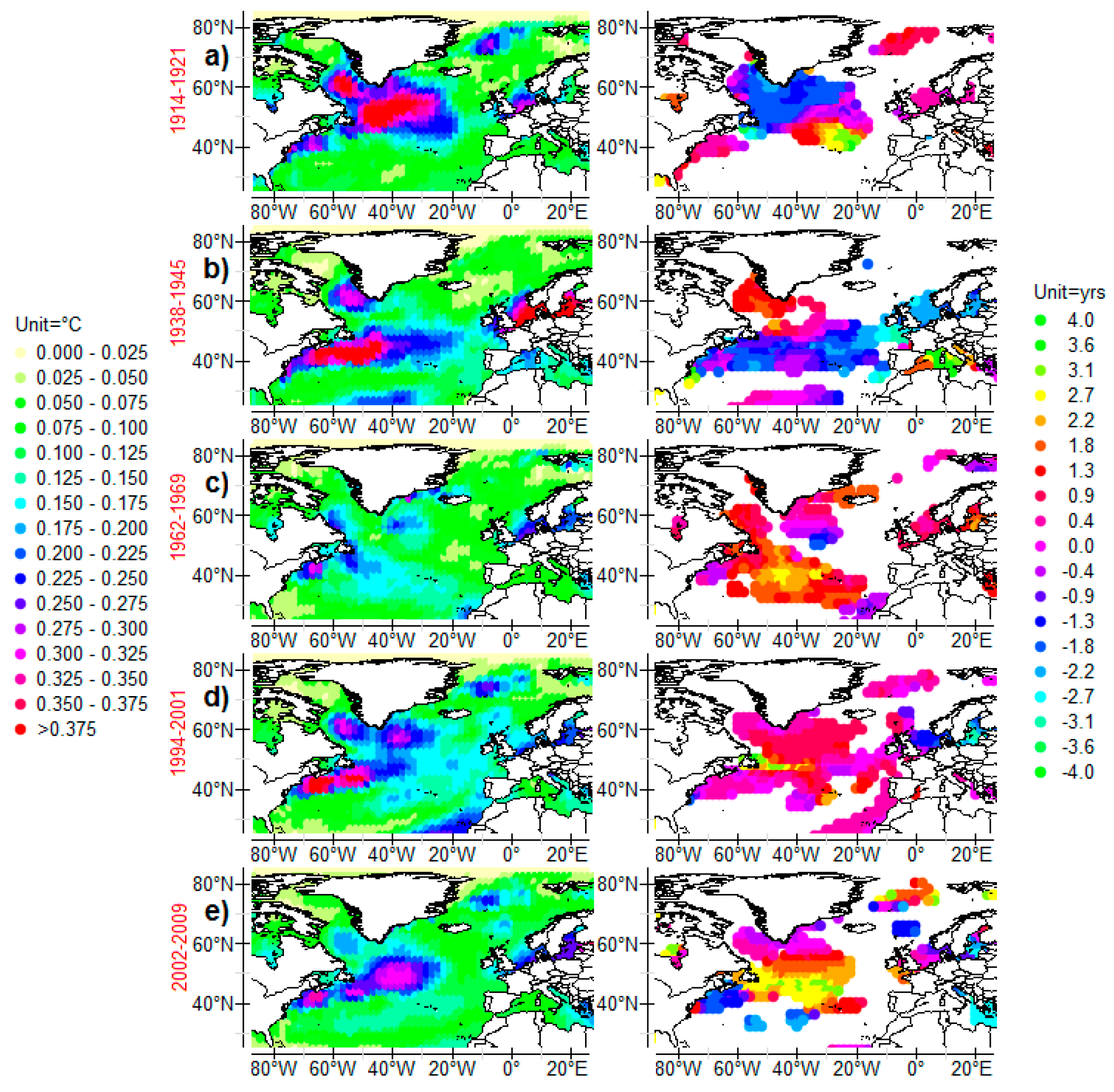
The pattern of SST anomalies in the North Atlantic (Figure 8) determines the amplitude and the phase of rainfall oscillation in Europe, in Western-Central Asia and in the north of Africa, at latitudes above the horse latitudes between 30° N and 35° N, extending to 85° E to the east (Figure 9). Four regions are particularly impacted, namely, Northwestern Europe, Western Europe, the states located around the Black Sea, and finally Uzbekistan and Kazakhstan. The deep continental penetration of the precipitation oscillation phenomenon demonstrates the alternation of synoptic high and low pressure systems stimulated and guided by the polar jet stream. Indeed, in the North Atlantic extra-tropical cyclones and anticyclones are formed from SST anomalies of four- and above all eight-year periods. The migration of depressions across Europe to Asia benefits from a low relief north of the Alps and the Himalayas.
The oscillation of precipitations disappears with SST anomaly, as occurred from 1954 to 1985 (Figure 8c and Figure 9c). Neither significant SST anomalies in the North Atlantic nor RRH anomalies in Europe and Western-Central Asia (eight-year period anomalies lower than 10%) are observable. In such a configuration, extra-tropical cyclones and anticyclones lose their anchorage and are produced more uniformly in space and time. Therefore, rainfall is evenly distributed during eight-year cycles.
Outside this period of very weak anomalies, the oscillation evolves according to the extension of the SST anomaly and the phase contrast within the anomaly. Comparison of the phases of SST and RRH anomalies indicates the origin of the extra-tropical cyclones that cause abundant precipitation, which depends on the cycle as will be seen farther. This means that the trajectory of the polar jet stream is closely conditioned by the pattern of the SST anomaly (somehow it is a coupling between the oceanic and the atmospheric Rossby waves via SST anomalies).
During 1906–1921, rainfall oscillation was mainly focused on Western-Central Asia, in Uzbekistan and Kazakhstan (Figure 9a). Both antinodes form a single SST anomaly of 0.4 °C between 40° N and 60° N, 60° W to 20° W, with two poles in opposite phase north and south of the anomaly. The RRH anomaly is in phase with the southernmost SST anomaly. When it is positive, baroclinic extra-tropical cyclones form along frontal zones of high temperature and dew point gradients. Synoptic extra-tropical cyclones migrate to Western-Central Asia between 40° N and 50° N. Therefore, it is the mean latitude of the northern hemisphere polar jet stream, under the influence of the positive southern SST anomaly. A negative southern SST anomaly promotes anticyclonic blocks. The ridge is guided by winds aloft, traveling across Europe and inducing droughts in Western-Central Asia. The distance between the SST anomaly and the impacted region is considerable, that is, nearly 8000 km, which supposes several synoptic systems may coexist between the SST and the RRH anomalies as may occur in the summer when successive anticyclones separated by depressions are formed over the North Atlantic, Europe and Western-Central Asia.
In contrast, during that period rainfall oscillation does not occur in Western Europe. Where positive and negative SST anomalies coexist in the North Atlantic, a depression is initiated when a wave develops on the front, that is, the boundary between cold and warm air masses generated by SST anomalies where temperature and dew point gradient are maximal. Cold and occluded fronts are guided by winds aloft, traveling from the northwest to southeast. They may produce extended zones of precipitation over Europe. This process continues when the polarity of the SST anomaly is reversed, so that rainfall does not oscillate in Western Europe.
During 1922–1937, as occurred later during 1954–1977, SST anomalies are small and weak, not exceeding 0.3 °C, and RRH anomalies in Europe and in Western-Central Asia do not exceed 15% (Figure 5b, Figure 8c and Figure 9c).
During 1938–1953 the SST anomaly intensified, reaching 0.4 °C, and extending eastward over the southwestern antinode between 40° N and 45° N so that the anomaly is almost monophasic (Figure 8b and Figure 9b). RRH anomalies intensify in Western Europe, too, in phase with the main SST anomaly. In the north of Europe, mainly the Scandinavia Peninsula including Finland, Iceland and the Faeroe Islands, rainfall oscillation strongly depends on the amplitude of SST in the North and Baltic seas reaching 0.35 °C. Concomitantly, the variability of rainfall increases in Northwestern Russia, between 30° E and 60° E, and in the south of Finland, where it reaches 20%. The RRH anomaly in the Northwestern Russia is in opposite phase relative to SST anomalies in the North and Baltic seas, which exhibits highs generated by negative SST anomalies that deviate the polar jet stream to the north, and depressions, too. In contrast, the track of depressions moves further south when lows are generated by positive SST anomalies, causing droughts in the north-western Russia.
This configuration is repeated during 1986–2001 in the North Atlantic, but this time with a nearly uniform phase, the dipole being strongly unbalanced, and with SST anomalies in the North and Baltic seas of lesser amplitude (Figure 8d and Figure 9d). RRH anomalies grow drastically in Western Europe. The north of France, the south of British Isles and the Benelux are mainly subject to rainfall oscillation, reaching 20% in relative value while being in phase with the main SST anomaly associated with the southwestern antinode off the Cape Hatteras.
The cycle 1994–2001 is particular insofar as the SST anomaly extends from 40° N to 65° N in latitude and from the coasts of North America to 30° W in longitude while being monophasic. In this way, rainfall oscillation occurs in the four locations indicated above, all RRH anomalies being in phase with the SST anomaly.
During 2002–2009 the phase of the SST anomaly differentiates from west to east, which mitigates RRH anomalies in Europe: in Western Europe they remain in phase with the SST anomaly off the Cape Hatteras, but in opposite phase in the Northwestern Europe, that is, the Northern Scandinavia peninsula and the Northern British Isles. A negative SST anomaly off the Cape Hatteras promotes anticyclonic blocks. The subsidence at their center in the lower portion of the troposphere and the circulation around mid-level ridges act to steer extra-tropical cyclones around their periphery, which promotes high pressure area (the Azores anticyclone) to the south and a low pressure area (the Icelandic Low), to the north. When cyclonic and anti-cyclonic systems last, Western Europe is affected by drought while the north is subject to flooding, and vice versa.
To summarize, rainfall oscillation occurs in Uzbekistan and Kazakhstan as soon as SST anomalies in the North Atlantic have sufficient amplitude because all parts of the anomaly may potentially produce lows or highs that, guided by the polar jet stream, induce either abundant rainfall focused on the northern Himalayas or droughts. Due to a lack of steering currents, upper level high or low pressure system is cut off. In contrast, rainfall oscillation in Western Europe reaches high amplitudes only if the phases of SST anomalies are well differentiated because it is mainly the extreme western portion of the western antinode that is involved. In such circumstances, RRH anomalies in opposite phase may appear in Northwestern and Western Europe, what abundant literature refers to as the North Atlantic Oscillation (NAO+ and NAO- depending on the sign of SST anomalies of the dipole).
3.2.11. Region of the Rio de la Plata
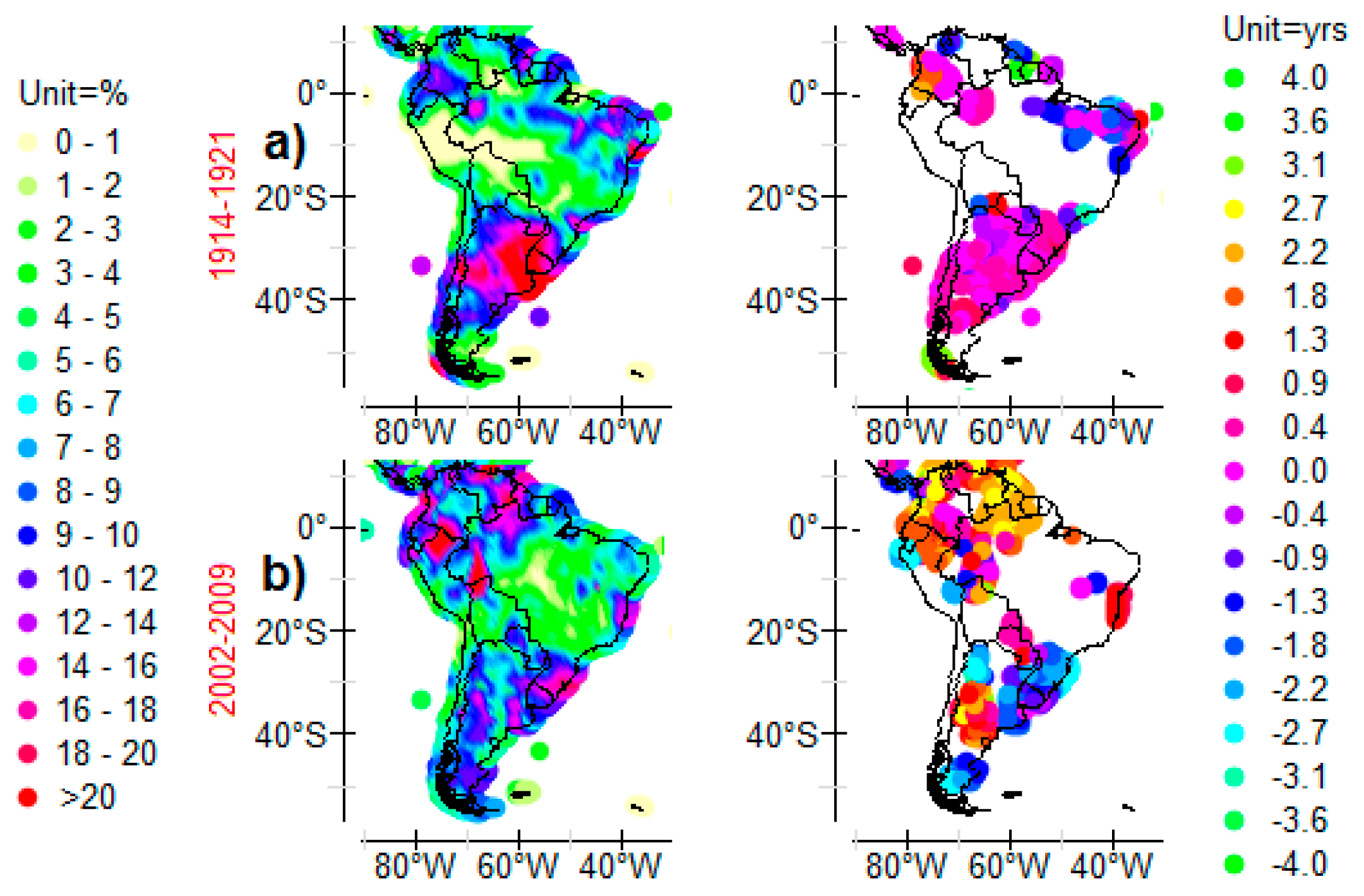
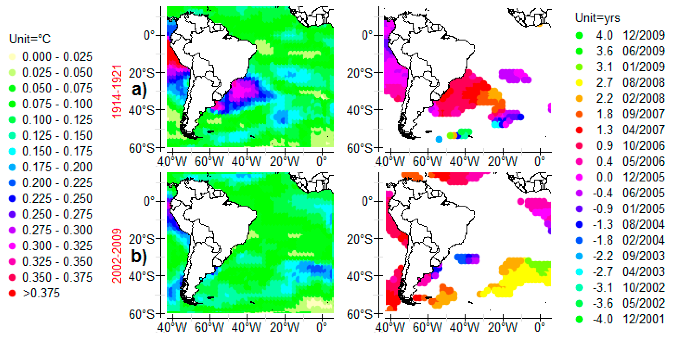
The region of the Rio de la Plata located where the Brazil Current leaves the continent to enter the subtropical gyre, that is, where oceanic Rossby waves resonate, is subject to rainfall oscillation whose relative amplitude may overreach 20%, as occurs during 1906–1921 (Figure 5h and Figure 10a). The rest of the time the RRH anomaly is about 10%, making it one of the most significant regions subject to rainfall oscillation in South America (Figure 10b). Two major surface currents collide off the Rio de la Plata, the northerly-flowing cold water Malvinas Current and the southerly-flowing warm water Brazil Current. Dragged by the Brazil current (i.e., the western boundary current of the South Atlantic subtropical gyre), Rossby waves propagate eastward then split into two brunches at 40° S and 50° S. RRH anomaly is in phase with the corresponding SST anomaly that extends eastward, between 20° S and 40° S (Figure 11). Positive SST anomaly at the western antinode promotes upper-level trough in phase with a low-level warm-core low. Subtropical cyclones may form if a strong dipole-blocking structure persists over the SST anomaly, which decreases wind shear across the region. Then, a low pressure area develops over the Amazon basin, and intensifies as it moves southeastward or eastward over open waters, establishing a very large closed circulation. The main regions exposed to locally heavy rains are Southern Brazil (Rio Grande do Sul), Uruguay and Northeastern Argentina. In contrast, a negative SST anomaly promotes anticyclonic blocks over the Amazon basin, causing dryer conditions in Uruguay and Northeastern Argentina mainly during austral winter.
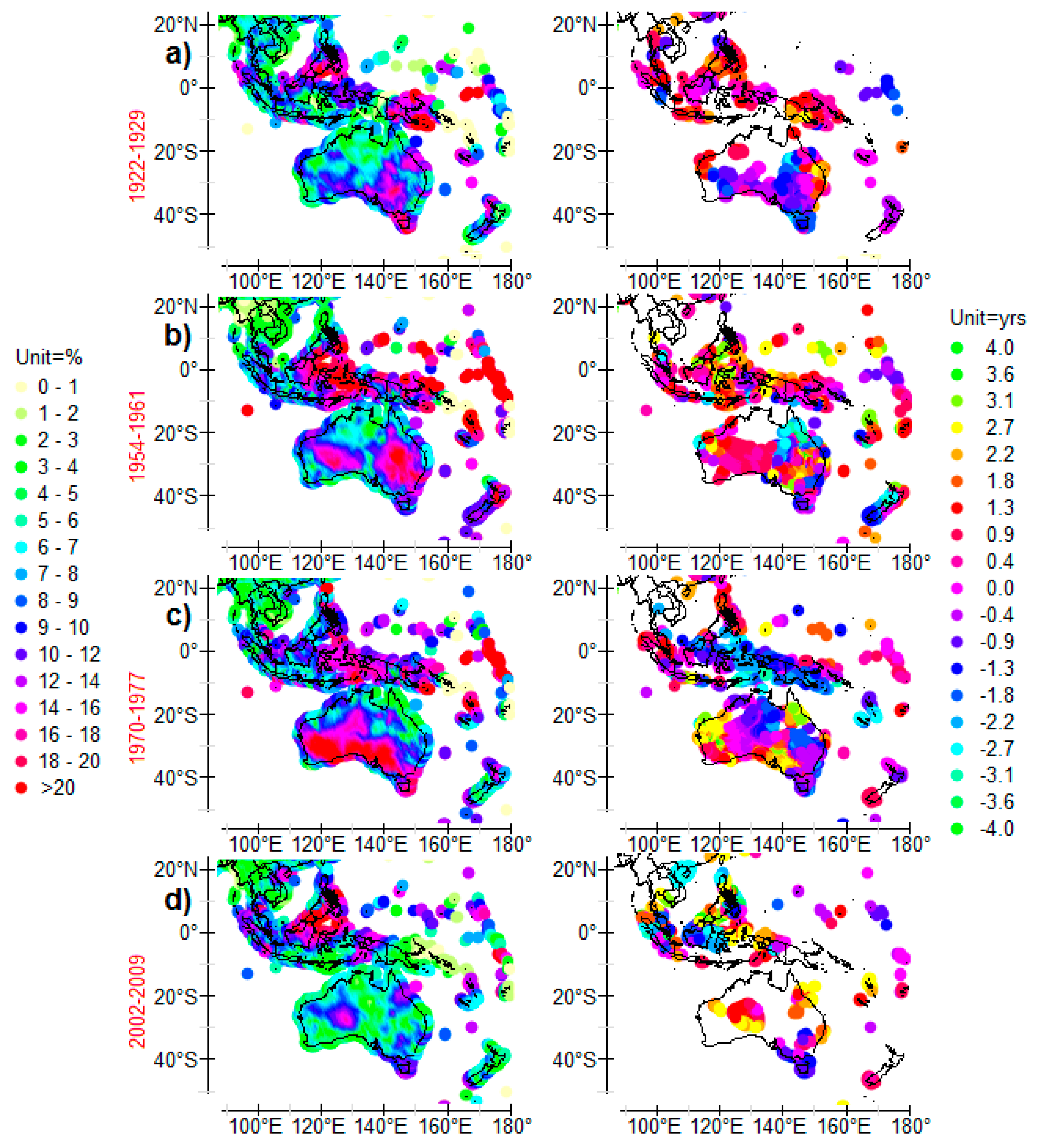
3.2.12. South-Western and South-Eastern Australia
Both Southwestern and Southeastern Australia are subject to severe rainfall oscillation. RRH anomalies may overreach 20% as occurred during 1946–1977 (Figure 5 and Figure 12b,c). They are in phase with the SST anomaly west of Australia (Figure 13). Located between 90° E and the western coast of Australia, and between 20° S and 40° S in latitude, the SST anomaly never exceeds 0.25 °C. However, stretching along the subtropical jet stream, it is extremely active and produces strong westward RRH anomalies according as it is positive or negative. The SST anomaly may split into northern and southern anomalies slightly out of phase, as occurred during 1954–1961 (Figure 13b). As shown from the phases of RRH and SST anomalies, the northern and the southern SST anomalies induce the southwestern and the southeastern RRH anomalies, respectively (Figure 12b).
Thus, lows produced from positive SST anomalies west of Australia are pulled towards cutoff lows. The same mechanisms are involved in the motion of highs produced from negative SST anomalies. Concerning RRH anomalies over the Southwestern Australia, cut-off lows and cutoff highs are formed against the Musgrave Ranges, a mountain range in Central Australia straddling the boundary of South Australia and the Northern Territory. They extend into Western Australia and the MacDonnell Ranges of the Northern Territory, a series of mountain ranges located in the center of Australia. As for RRH anomalies over the south-eastern portion of the continent, cutoff lows and cutoff highs are formed against the East Australian Cordillera.
3.2.13. South-Eastern Asia
Although exhibiting lower RRH anomalies, Southeast Asia is subject to northeastward migration of tropical cyclones as occurs in Southeastern North America. Here, positive SST anomalies in the Northwestern Pacific seem less decisive for moving of tropical cyclones to the north by merging two low pressure systems.
4. Discussion
The joint study of the amplitude and the phase of both RRH and SST anomalies in the 5–10 year band on a worldwide scale and during almost one century discloses the mechanisms leading to the formation of high and low atmospheric pressure systems, which helps answer a number of issues regarding the characteristics of ocean-atmosphere interactions in a changing climate. The mechanisms invoked seem plausible because the robustness of the hypotheses is put to severe test given the great variety in the space and time of the analyzed situations. Furthermore, the location and evolution over time of SST anomalies suggest that they result from the dynamics of subtropical ocean gyres.
However, a key issue remains unresolved. Has the oscillation in the 5–10 year band, which has been experiencing an upsurge in Europe and America since the end of the 20th century, been a consequence of anthropogenic climate warming? More generally, what is the driver of the four- and eight-year period SST anomalies?
The first issue to be considered is the possible link between four- and eight-year period SST anomalies, and long-period RFWs. Because long-period Rossby waves are non-dispersive, their wavelength is proportional to the period. A search path that should be promising relies on the modulated response to periodical forcing of subtropical gyres, supposing long-wavelength Rossby waves wrap around the gyres. This is what the Rossby wave theory provides when the variation in the Coriolis Effect with the mean radius of the gyres is considered, a way of generalizing a well-known property of Rossby waves as they propagate along a parallel while the Coriolis Effect varies with the latitude.
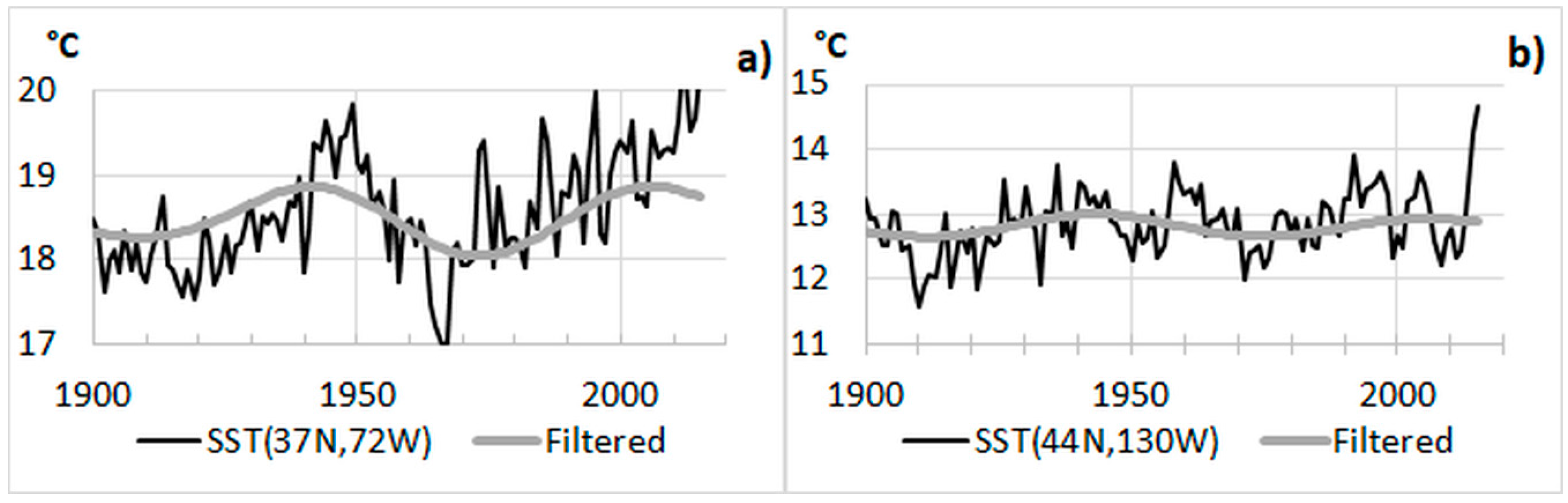
The representation of the SST anomaly, filtered in the 48–96 year band, where the Gulf Stream leaves the North American continent at 37° N, 72° W shows that the low amplitude of the eight-year period SST anomaly observed in 1962–1969 in Western Europe and in Southeastern North America coincides with a low amplitude of the long-period SST anomaly (Figure 5f and Figure 14a). Furthermore, the high amplitude of the eight-year period SST anomaly that occurs before and after this period of lull coincides with the high amplitude of the SST anomaly of average period 64 years.
By contrast, the link between the amplitudes of the eight-year period and long-period SST anomalies is not clear for the other subtropical gyres where the amplitude of the SST anomaly of average period 64 years is weak (Figure 5c and Figure 14b). As a result of the potent thermohaline circulation, which reinforces the northeastern antinodes of RFWs, possibly a positive feedback loop is enhanced around the North Atlantic subtropical gyre. Thus, an increase in long-period oscillation of the geostrophic current velocity around the gyre and, therefore, of the heat flux transported poleward, may arouse shorter period oscillations at mid-latitudes.
Further researches are required to confirm or disprove the possible link between the amplitude of the rainfall oscillation, and more particularly the frequency and the amplitude of subtropical cyclones, and the SST anomalies of short and longer periods at mid-latitudes. However, the cyclical nature of the amplitude of the rainfall oscillation in the band 5–10 years rather goes in the direction of a resonant phenomenon, whereas the anthropogenic forcing is typically non-resonant. In the latter case, the amplitude of the oscillation should continue to increase during the next decades, whereas it should decrease in the case of long-period cyclicality unless the two phenomena compensate each other.
Acknowledgments
We thank the associated editor and the reviewers for their helpful comments.
Conflicts of Interest
The author declares no conflict of interest.
References
- Kapala, A.; Mächel, H.; Flohn, H. Behaviour of the centres of action above the Atlantic since 1881. Part II: Associations with regional climate anomalies. Int. J. Climatol. 1998, 18, 23–36. [Google Scholar] [CrossRef]
- Baines, P.G.; Folland, C.K. Evidence for a rapid global climate shift across the late 1960s. J. Clim. 2007, 20, 2721–2744. [Google Scholar] [CrossRef]
- Pokrovsky, O.M. European rain rate modulation enhanced by changes in the NAO and atmospheric circulation regimes. Comput. Geosci. 2009, 35, 897–906. [Google Scholar] [CrossRef]
- Rodó, X.; Baert, E.; Comin, F.A. Variations in seasonal rainfall in Southern Europe during the present century: Relationships with the North Atlantic Oscillation and the El Niño-Southern Oscillation. Clim. Dyn. 1997, 13, 275–284. [Google Scholar] [CrossRef]
- Brandimarte, L.; Di Baldassarre, G.; Bruni, G.; D’Odorico, P.; Montanari, A. Relation Between the North-Atlantic Oscillation and Hydroclimatic Conditions in Mediterranean Areas. Water Resour. Manag. 2011, 25, 1269–1279. [Google Scholar] [CrossRef]
- Munoz-Díaz, D.; Rodrigo, F.S. Impacts of the North Atlantic Oscillation on the probability of dry and wet winters in Spain. Clim. Res. 2004, 27, 33–43. [Google Scholar] [CrossRef]
- Santos, J.A.; Corte-Real, J.; Leite, S.M. Weather regimes and their connection to the winter rainfall in Portugal. Int. J. Climatol. 2005, 25, 33–50. [Google Scholar] [CrossRef]
- Millán, M.M.; Estrela, M.J.; Miró, J. Rainfall components: Variability and spatial distribution in a Mediterranean area (Valencia region). J. Clim. 2005, 18, 2682–2705. [Google Scholar] [CrossRef]
- Gallego, M.C.; García, J.A.; Vaquero, J.M. The NAO signal in daily rainfall series over the Iberian Peninsula. Clim. Res. 2005, 29, 103–109. [Google Scholar] [CrossRef]
- Barrera, A.; Barriendos, M.; Llasat, M.C. Extreme flash floods in Barcelona County. Adv. Geosci. 2005, 2, 111–116. [Google Scholar] [CrossRef]
- Andreo, B.; Jiménez, P.; Durán, J.J.; Carrasco, F.; Vadillo, I.; Mangin, A. Climatic and hydrological variations during the last 117–166 years in the south of the Iberian Peninsula, from spectral and correlation analyses and continuous wavelet analyses. J. Hydrol. 2006, 324, 24–39. [Google Scholar] [CrossRef]
- Luque-Espinar, J.A.; Chica-Olmo, M.; Pardo-Igúzquiza, E.; García-Soldado, M.J. Influence of climatological cycles on hydraulic heads across a Spanish aquifer. J. Hydrol. 2008, 354, 33–52. [Google Scholar] [CrossRef]
- Lorenzo, M.N.; Taboada, J.J.; Gimeno, L. Links between circulation weather types and teleconnection patterns and their influence on precipitation patterns in Galicia (NW Spain). Int. J. Climatol. 2008, 28, 1493–1505. [Google Scholar] [CrossRef]
- Lopez-Bustins, J.-A.; Martin-Vide, J.; Sanchez-Lorenzo, A. Iberia winter rainfall trends based upon changes in teleconnection and circulation patterns. Glob. Planet. Chang. 2008, 63, 171–176. [Google Scholar] [CrossRef]
- Delitala, A.M.S.; Cesari, D.; Chessa, P.A.; Ward, M.N. Precipitation over Sardinia (Italy) during the 1946–1993 rainy seasons and associated large-scale climate variations. Int. J. Climatol. 2000, 20, 519–541. [Google Scholar] [CrossRef]
- Cislaghi, M.; De Michele, C.; Ghezzi, A.; Rosso, R. Statistical assessment of trends and oscillations in rainfall dynamics: Analysis of long daily Italian series. Atmos. Res. 2005, 77, 188–202. [Google Scholar] [CrossRef]
- Dixon, H.; Lawler, D.M.; Shamseldin, A.Y. Streamflow trends in western Britain. Geophys. Res. Lett. 2006, 33, L19406. [Google Scholar] [CrossRef]
- Hannaford, J.; Marsh, T.J. High-flow and flood trends in a network of undisturbed catchments in the UK. Int. J. Climatol. 2008, 28, 1325–1338. [Google Scholar] [CrossRef]
- Kiely, G. Climate change in Ireland from precipitation and streamflow observations. Adv. Water Resour. 1999, 23, 141–151. [Google Scholar] [CrossRef]
- Massei, N.; Durand, A.; Deloffre, J.; Dupont, J.P.; Valdes, D.; Laignel, B. Investigating possible links between the North Atlantic Oscillation and rainfall variability in Northwestern France over the past 35 years. J. Geophys. Res. D Atmos. 2007, 112, D09121. [Google Scholar] [CrossRef]
- Massei, N.; Laignel, B.; Deloffre, J.; Mesquita, J.; Motelay, A.; Lafite, R.; Durand, A. Long-term hydrological changes of the Seine River flow (France) and their relation to the North Atlantic Oscillation over the period 1950–2008. Int. J. Climatol. 2010, 30, 2146–2154. [Google Scholar] [CrossRef]
- Pinault, J.L. Global warming and rainfall oscillation in the 5–10 yr band in Western Europe and Eastern North America. Clim. Chang. 2012, 114, 621–650. [Google Scholar] [CrossRef]
- Wang, C.; Enfield, D.B.; Lee, S.-K.; Landsea, C.W. Influences of the Atlantic warm pool on western hemisphere summer rainfall and Atlantic hurricanes. J. Clim. 2006, 19, 3011–3028. [Google Scholar] [CrossRef]
- Wang, C.; Lee, S.-K.; Enfield, D.B. Climate response to anomalously large and small Atlantic warm pools during the summer. J. Clim. 2008, 21, 2437–2450. [Google Scholar] [CrossRef]
- Hu, Q.; Feng, S. Variation of the North American summer monsoon regimes and the Atlantic multidecadal oscillation. J. Clim. 2008, 21, 2371–2383. [Google Scholar] [CrossRef]
- Collins, M. Evidence for Changing Flood Risk in New England Since the Late 20th Century. J. Am. Water Resour. Assoc. 2009, 45, 279–290. [Google Scholar] [CrossRef]
- Massei, N.; Laignel, B.; Rosero, E.; Motelay, A.; Deloffre, J.; Yang, Z.-L.; Rossi, A. A wavelet approach to the intra-annual to pluridecennal variability of streamflow in the Mississippi river basin from 1934 to 1998. Int. J. Climatol. 2011, 31, 31–43. [Google Scholar] [CrossRef]
- Pinault, J.-L.; Amraoui, N.; Golaz, C. Groundwater-induced flooding in macropore-dominated hydrological system in the context of climate changes. Water Resour. Res. 2005, 41, W05001. [Google Scholar] [CrossRef]
- Weng, H.; Lau, K.-M. Wavelets, period doubling, and time-frequency localization with application to organization of convection over the tropical western Pacific. J. Atmos. Sci. 1994, 51, 2523–2541. [Google Scholar] [CrossRef]
- Gu, D.; Philander, S.G.H. Secular changes of annual and interannual variability in the Tropics during the past century. J. Clim. 1995, 8, 864–876. [Google Scholar] [CrossRef]
- Wang, B.; Wang, Y. Temporal structure of the Southern Oscillation as revealed by waveform and wavelet analysis. J. Clim. 1996, 9, 1586–1598. [Google Scholar] [CrossRef]
- Gamage, N.; Blumen, W. Comparative analysis of low level cold fronts: Wavelet, Fourier, and empirical orthogonal function decompositions. Mon. Weather Rev. 1993, 121, 2867–2878. [Google Scholar] [CrossRef]
- Baliunas, S.; Frick, P.; Sokoloff, D.; Soon, W. Time scales and trends in the central England temperature data (1659–1990): A wavelet analysis. Geophys. Res. Lett. 1997, 24, 1351–1354. [Google Scholar] [CrossRef]
- Meyers, S.D.; Kelly, B.G.; O’Brien, J.J. An introduction to wavelet analysis in oceanography and meteorology: With application to the dispersion of Yanai waves. Mon. Weather Rev. 1993, 121, 2858–2866. [Google Scholar] [CrossRef]
- Liu, P.C. Wavelet spectrum analysis and ocean wind waves. In Wavelets in Geophysics; Foufoula-Georgiou, E., Kumar, P., Eds.; Academic Press: Cambridge, MA, USA, 1994; pp. 151–166. [Google Scholar]
- Farge, M. Wavelet transforms and their applications to turbulence. Annu. Rev. Fluid Mech. 1992, 24, 395–457. [Google Scholar] [CrossRef]
- Torrence, C.; Compo, G.P. A practical guide for wavelet analysis. Bull. Am. Meteorol. Soc. 1998, 79, 61–78. [Google Scholar] [CrossRef]
- Extended Reconstructed Sea Surface Temperatures, Version 3 (ERSST.v3) from the National Oceanic and Atmospheric Administration (NOAA). Available online: http://www.emc.ncep.noaa.gov/research/cmb/sst_analysis/ (accessed on 1 September 2017).
- Monthly Rainfall Data from the Climatic Research Unit (CRU). Available online: http://badc.nerc.ac.uk/data/cru/ (accessed on 1 September 2017).
- Monthly Southern Oscillation Index from the National Centre for Atmospheric Research (NCAR). Available online: http://www.cgd.ucar.edu/cas/catalog/climind/soi.html (accessed on 1 September 2017).
- Okoola, R.E.; Ambenje, P.G. Transition from the Southern to the Northern Hemisphere summer of zones of active convection over the Congo Basin. Meteorol. Atmos. Phys. 2003, 84, 255–265. [Google Scholar] [CrossRef]
- Washington, R.; James, R.; Pearce, H.; Pokam, W.M.; Moufouma-Okia, W. Congo Basin rainfall climatology: Can we believe the climate models? Philos. Trans. R. Soc. B 2013, 368, 20120296. [Google Scholar] [CrossRef] [PubMed]
- Todd, M.C.; Washington, R. Climate variability in central equatorial Africa: Influence from the Atlantic sector. Geophys. Res. Lett. 2004, 31, 203–218. [Google Scholar] [CrossRef]
- Okumura, Y.; Xie, S.P. Some overlooked features of tropical Atlantic climate leading to a new Nino-Like phenomenon. J. Clim. 2006, 19, 5859–5874. [Google Scholar] [CrossRef]
- Balas, N.; Nicholson, S.E.; Klotter, D. The relationship of rainfall variability in West Central Africa to sea-surface temperature fluctuations. Int. J. Climatol. 2007, 27, 1335–1349. [Google Scholar] [CrossRef]
- Dezfuli, A.K.; Nicholson, S.E. The relationship of rainfall variability in western equatorial Africa to the tropical oceans and atmospheric circulation. Part II: The boreal autumn. J. Clim. 2013, 26, 66–84. [Google Scholar] [CrossRef]
- Nicholson, S.E.; Dezfuli, A.K. The relationship of rainfall variability in western equatorial Africa to the tropical oceans and atmospheric circulation. Part I: The boreal spring. J. Clim. 2013, 26, 45–65. [Google Scholar] [CrossRef]
- Gill, A.E. Atmosphere–Ocean Dynamics; International Geophysics Series, 30; Academic Press: Cambridge, MA, USA, 1982; p. 662. [Google Scholar]
- Pinault, J.L. Long wave resonance in tropical oceans and implications on climate: The Pacific Ocean. Pure Appl. Geophys. 2015, 173, 2119–2145. [Google Scholar] [CrossRef]
- Cipollini, P.; Cromwell, D.; Quartly, G.D.; Challenor, P.G. Chapter 6 Remote sensing of oceanic extratropical Rossby waves. Elsevier Oceanogr. Ser. 2000, 63, 99–123. [Google Scholar] [CrossRef]
- Pinault, J.L. Long wave resonance in tropical oceans and implications on climate: The Atlantic Ocean. Pure Appl. Geophys. 2013, 170, 1913–1930. [Google Scholar] [CrossRef]
- Explain with Realism Climate Variability. Available online: http://climatorealist.neowordpress.fr/resonant-rainfall-oscillation/ (accessed on 11 June 2015).
- Pinault, J.L. Modulated response of subtropical gyres: Positive feedback, subharmonic modes, resonant solar and orbital forcing. Ocean Dyn. 2018. submitted for publication. [Google Scholar]
Figure 1.
Fourier power spectrum of the Southern Oscillation Index (SOI) from 1866 to 2016 and the confidence spectrum assuming a red-noise with a lag-1 .
Figure 1.
Fourier power spectrum of the Southern Oscillation Index (SOI) from 1866 to 2016 and the confidence spectrum assuming a red-noise with a lag-1 .

Figure 2.
Cross-wavelet power (top) and coherence phase (bottom) of (reduced rainfall height (RRH), -SOI), scale-averaged over the 5–10 year band representative of the eight-year period, time-averaged over 1901–2009.
Figure 2.
Cross-wavelet power (top) and coherence phase (bottom) of (reduced rainfall height (RRH), -SOI), scale-averaged over the 5–10 year band representative of the eight-year period, time-averaged over 1901–2009.

Figure 3.
Cross-wavelet power (top) and coherence phase (bottom) of (RRH, sea surface temperature (SST)0N, 10E) scale-averaged over the 8–16 month band representative of the annual period, time-averaged over 1901–2009.
Figure 3.
Cross-wavelet power (top) and coherence phase (bottom) of (RRH, sea surface temperature (SST)0N, 10E) scale-averaged over the 8–16 month band representative of the annual period, time-averaged over 1901–2009.

Figure 4.
Cross-wavelet power (top) and coherence phase (bottom) of (RRH, SST14N, 60E) scale-averaged over the 5–7 month band representative of the semi-annual period, time-averaged over 1901–2009. A continuous Morlet wavelet transform is used.
Figure 4.
Cross-wavelet power (top) and coherence phase (bottom) of (RRH, SST14N, 60E) scale-averaged over the 5–7 month band representative of the semi-annual period, time-averaged over 1901–2009. A continuous Morlet wavelet transform is used.
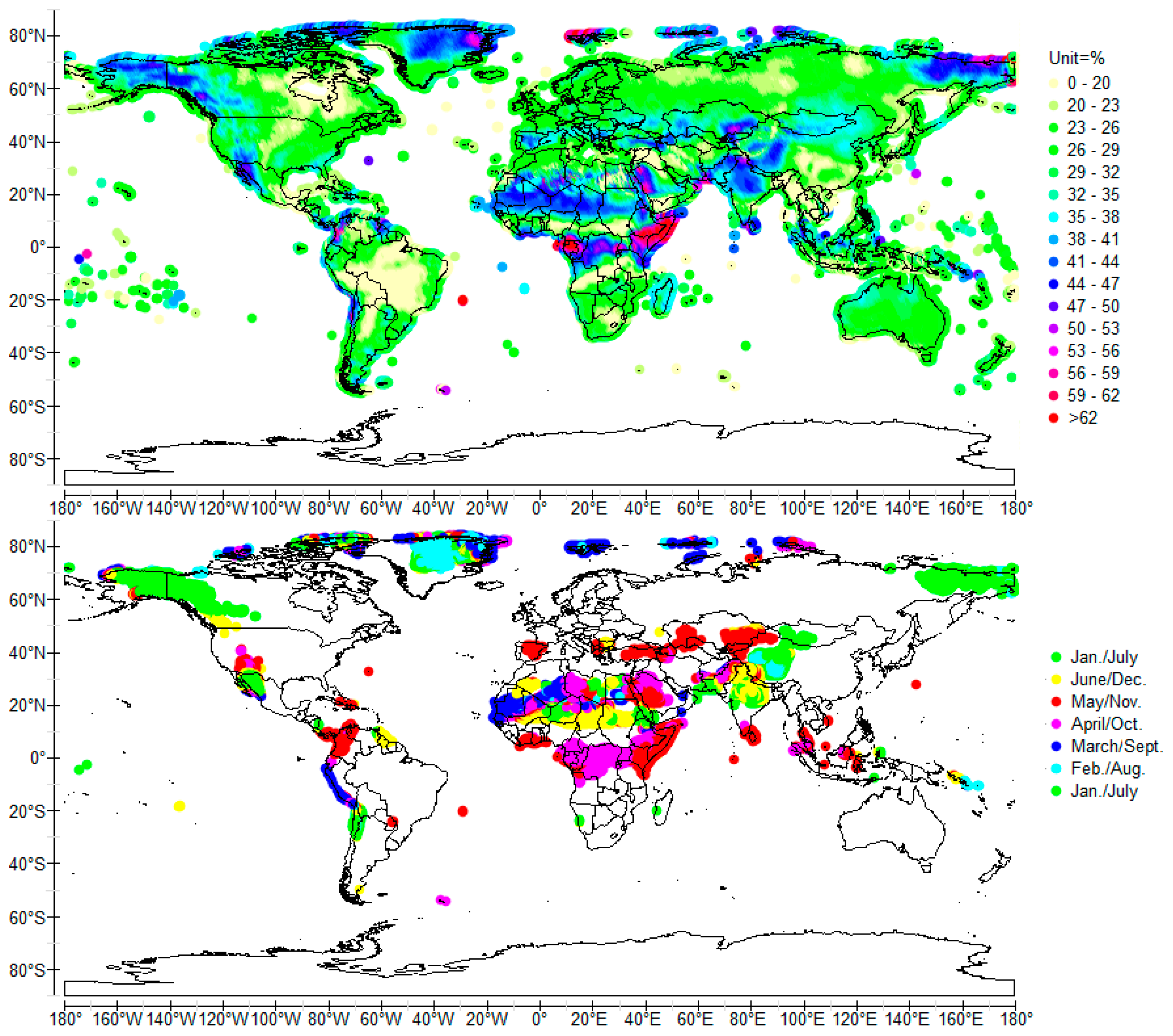
Figure 5.
Amplitude (on the left) and phase relative to the El Niño mature in 11/1997 (on the right) of the cross-wavelet power of (SST, -SOI) (a,b), and (RRH, -SOI) (c,d). Both are scale-averaged over the 3.5–4.5 year band.
Figure 5.
Amplitude (on the left) and phase relative to the El Niño mature in 11/1997 (on the right) of the cross-wavelet power of (SST, -SOI) (a,b), and (RRH, -SOI) (c,d). Both are scale-averaged over the 3.5–4.5 year band.
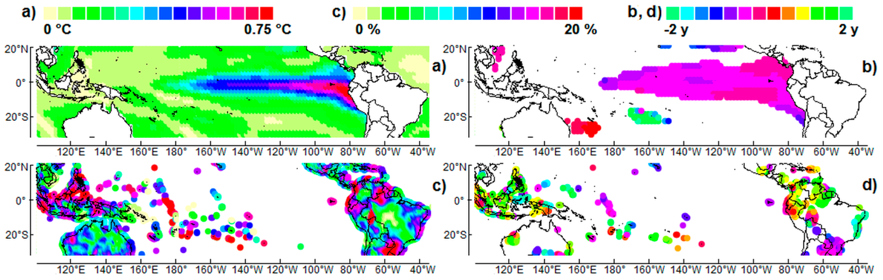
Figure 6.
Cross-wavelet power of (RRH, -SOI) (on the left) and coherence phase (on the right) scale-averaged over the 5–10 year band. The time is divided into intervals of eight years since 1906.
Figure 6.
Cross-wavelet power of (RRH, -SOI) (on the left) and coherence phase (on the right) scale-averaged over the 5–10 year band. The time is divided into intervals of eight years since 1906.
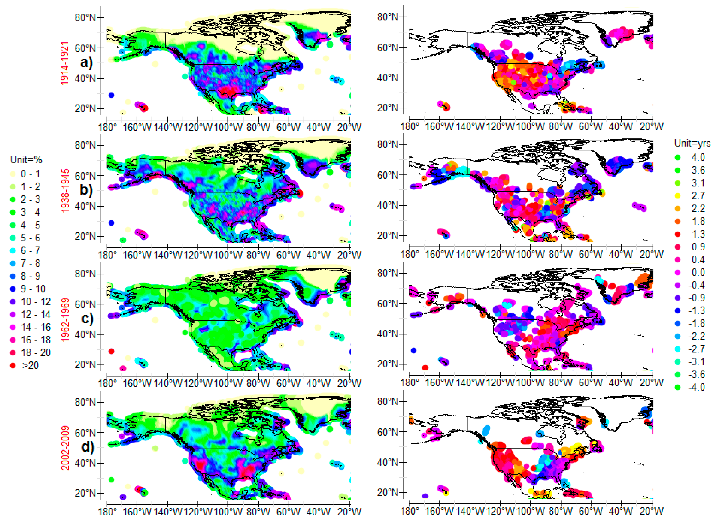
Figure 7.
Cross-wavelet power of (SST, -SOI) (on the left) and coherence phase (on the right) scale-averaged over the 5–10 year band.
Figure 7.
Cross-wavelet power of (SST, -SOI) (on the left) and coherence phase (on the right) scale-averaged over the 5–10 year band.
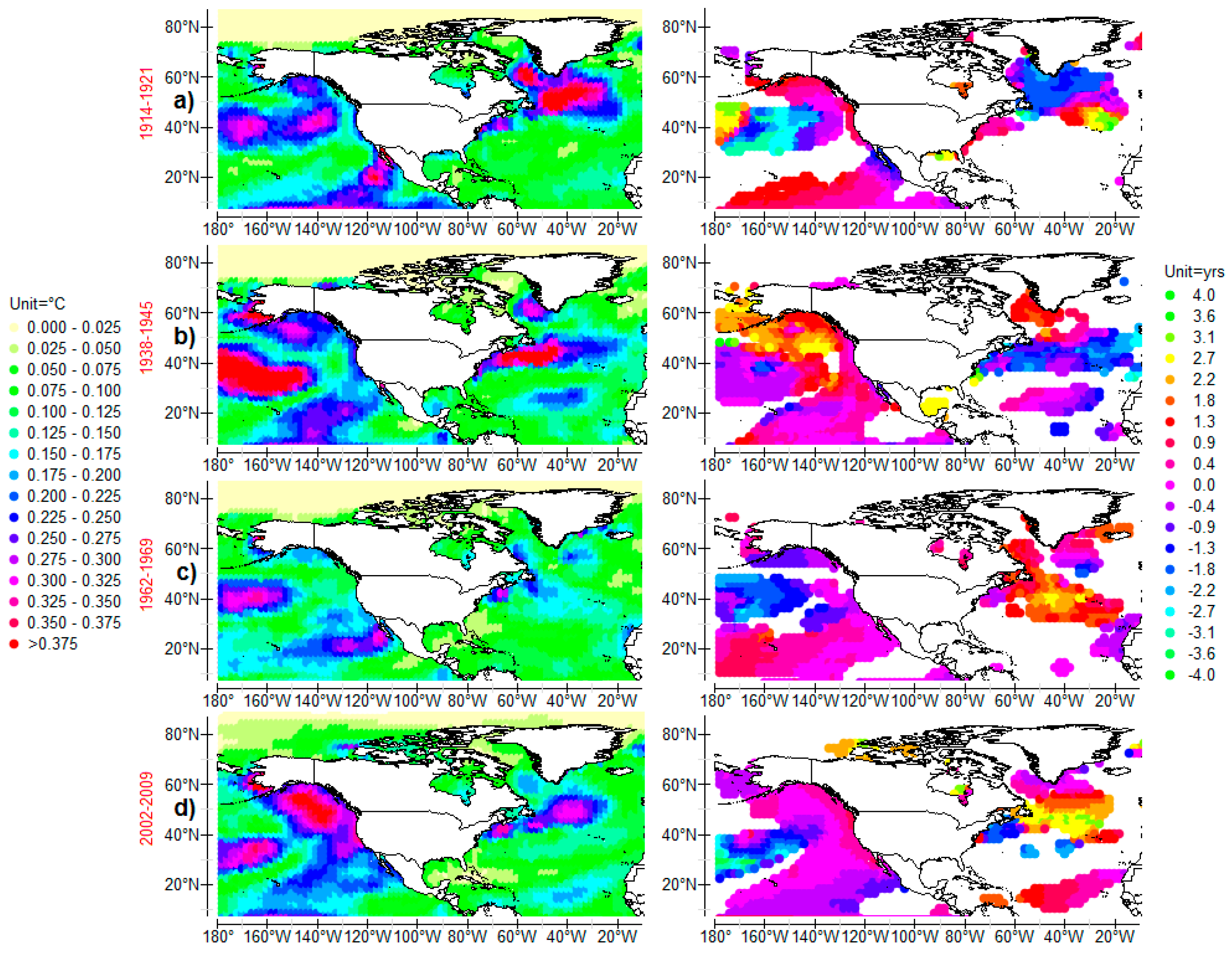
Figure 8.
Cross-wavelet power of (SST, -SOI) (on the left) and coherence phase (on the right) scale-averaged over the 5–10 year band.
Figure 8.
Cross-wavelet power of (SST, -SOI) (on the left) and coherence phase (on the right) scale-averaged over the 5–10 year band.

Figure 9.
Cross-wavelet power of (RRH, -SOI) (on the left) and coherence phase (on the right) scale-averaged over the 5–10 year band.
Figure 9.
Cross-wavelet power of (RRH, -SOI) (on the left) and coherence phase (on the right) scale-averaged over the 5–10 year band.
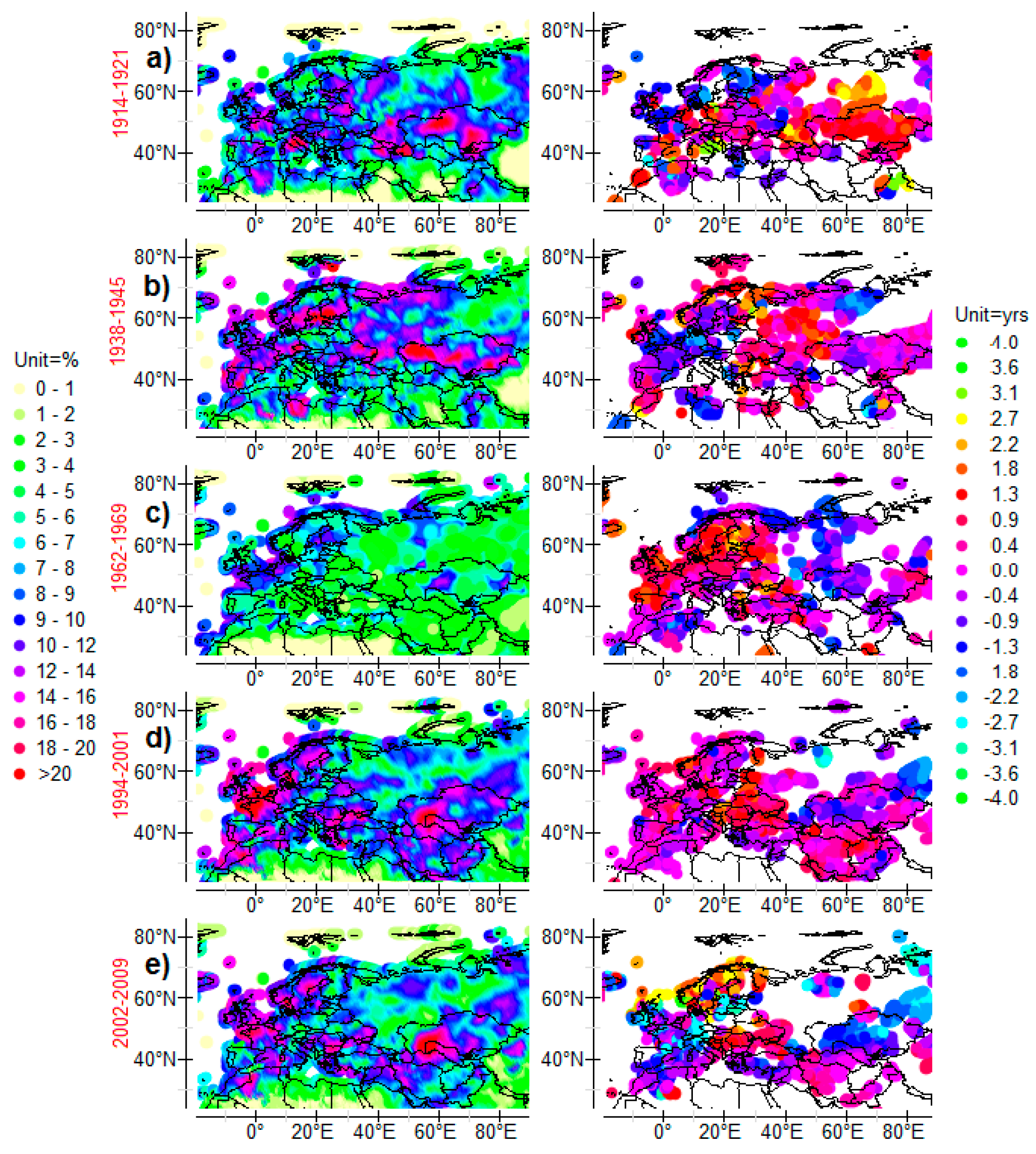
Figure 10.
Cross-wavelet power of (RRH, -SOI) (on the left) and coherence phase (on the right) scale-averaged over the 5–10 year band.
Figure 10.
Cross-wavelet power of (RRH, -SOI) (on the left) and coherence phase (on the right) scale-averaged over the 5–10 year band.

Figure 11.
Cross-wavelet power of (SST, -SOI) (on the left) and coherence phase (on the right) scale-averaged over the 5–10 year band.
Figure 11.
Cross-wavelet power of (SST, -SOI) (on the left) and coherence phase (on the right) scale-averaged over the 5–10 year band.

Figure 12.
Cross-wavelet power of (RRH, -SOI) (on the left) and coherence phase (on the right) scale-averaged over the 5–10 year band.
Figure 12.
Cross-wavelet power of (RRH, -SOI) (on the left) and coherence phase (on the right) scale-averaged over the 5–10 year band.

Figure 13.
Cross-wavelet power of (SST, -SOI) (on the left) and coherence phase (on the right) scale-averaged over the 5–10 year band.
Figure 13.
Cross-wavelet power of (SST, -SOI) (on the left) and coherence phase (on the right) scale-averaged over the 5–10 year band.
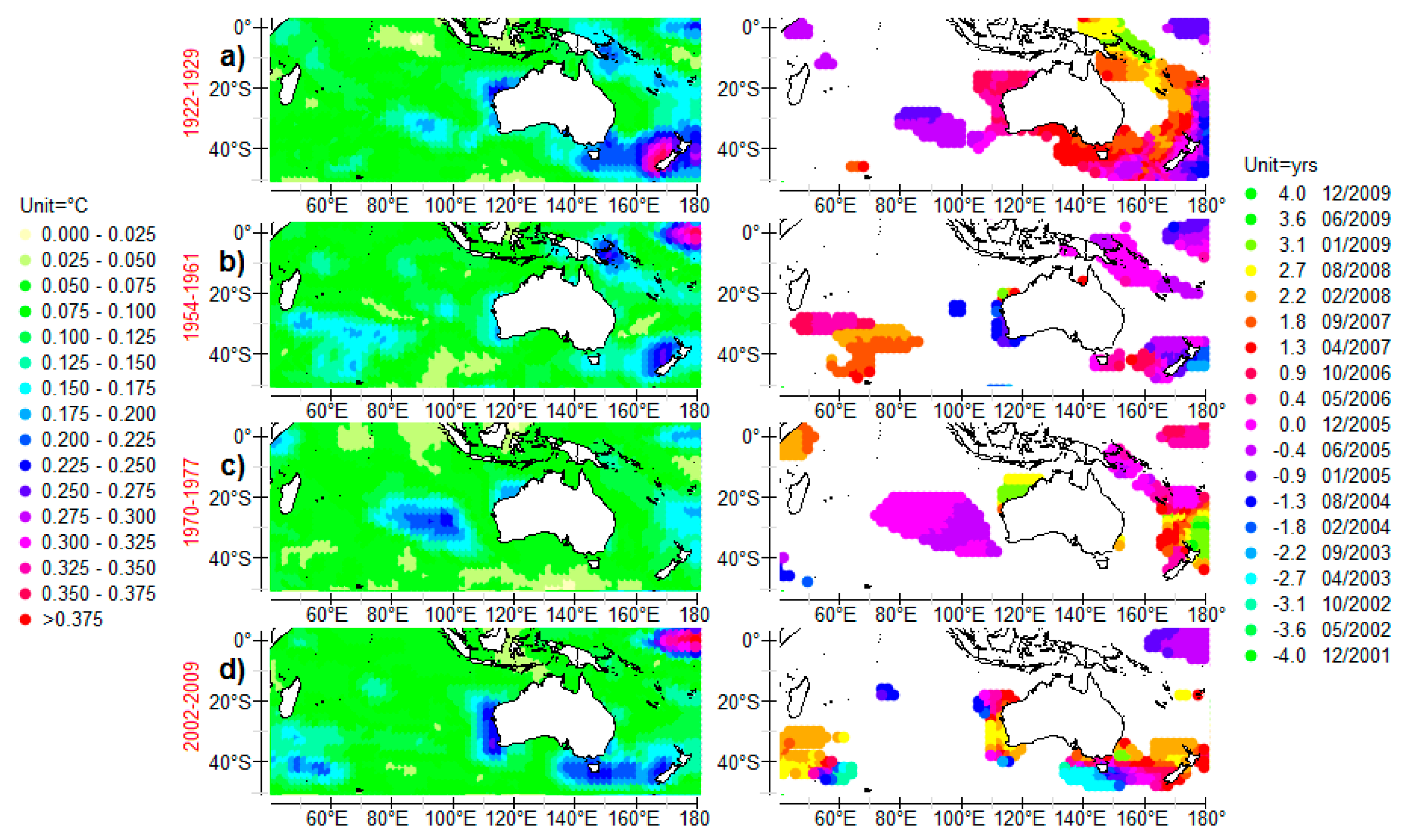
Figure 14.
SST at (a) 37° N, 72° W and (b) 44° N, 130° W, unfiltered and filtered in the 48–96 year band.
Figure 14.
SST at (a) 37° N, 72° W and (b) 44° N, 130° W, unfiltered and filtered in the 48–96 year band.
© 2018 by the author. Licensee MDPI, Basel, Switzerland. This article is an open access article distributed under the terms and conditions of the Creative Commons Attribution (CC BY) license (http://creativecommons.org/licenses/by/4.0/).
Share and Cite
MDPI and ACS Style
Pinault, J.-L. Regions Subject to Rainfall Oscillation in the 5–10 Year Band. Climate 2018, 6, 2. https://doi.org/10.3390/cli6010002
AMA Style
Pinault J-L. Regions Subject to Rainfall Oscillation in the 5–10 Year Band. Climate. 2018; 6(1):2. https://doi.org/10.3390/cli6010002
Chicago/Turabian StylePinault, Jean-Louis. 2018. "Regions Subject to Rainfall Oscillation in the 5–10 Year Band" Climate 6, no. 1: 2. https://doi.org/10.3390/cli6010002
Note that from the first issue of 2016, this journal uses article numbers instead of page numbers. See further details here.