
Adaption to Climate Change through Fallow Rotation in the U.S. Pacific Northwest

1
Department of Applied Economics, Oregon State University, Corvallis, OR 97330, USA
2
Department of Geography and Environmental Sustainability, University of Oklahoma, Norman, OK 73019, USA
3
Department of Agricultural Economics, Texas A&M University, College Station, TX 77843, USA
*
Author to whom correspondence should be addressed.
Climate 2017, 5(3), 64; https://doi.org/10.3390/cli5030064
Submission received: 11 July 2017
/
Revised: 7 August 2017
/
Accepted: 8 August 2017
/
Published: 15 August 2017
(This article belongs to the Special Issue Strategies for Climate Mitigation and Adaptation in Agriculture)
Abstract
:In this paper, we study the use of wheat land fallow production systems as a climate change adaptation strategy. Using data from the U.S. Census of Agriculture, we find that fallow is an important adaption strategy for wheat farms in the U.S. Pacific Northwest region. In particular, we find that a warmer and wetter climate increases the share of fallow in total cropland and thus reduces cropland in production. Our simulations project that, on average by 2050, the share of fallow (1.5 million acres in 2012) in the U.S. Pacific Northwest region will increase by 1.3% (0.12 million acres) under a medium climate change scenario and by 1.8% (0.16 million acres) under a high climate change scenario.
1. Introduction
Wheat is the most widely grown cereal grain, occupying 16% of global arable land [1]. Wheat also provides about 19% of global human calories and 21% of the protein [2]. Climate change may disrupt wheat yields with the Intergovernmental Panel on Climate Change (IPCC) showing estimates as large as a 5% reduction in the absence of adaptation [3].
A growing body of literature has examined climate change adaptation. Adaptation strategies include alterations in planting dates, irrigation technologies, agricultural land use, crop mix and cropping systems, and the use of crop insurance [4,5,6,7,8,9,10,11,12]. Another possible adaptation strategy is the use of fallow, where land is left idle to accumulate moisture as a means of adapting to dry conditions [13,14,15].
In this paper, we investigate the extent to which fallow is an observed adaptation strategy to drier climates and the extent to which it might change under climate change. We will examine the observed relationship of fallow share to climate using farm level census data for wheat farms in the U.S. Pacific Northwest (PNW) region. We will also project the consequences of climate change for fallow share using climate projections from 20 global climate models in the Coupled Model Intercomparison Project Phase 5 (CMIP5).
In the PNW 4.23 million acres of wheat were planted in 2016 and 75% of the planted wheat was winter wheat [16]. Most of that wheat was rainfed and grown between the Cascades and the Northern Rocky Mountains. There are four major cereal cropping systems in the region: (1) the rotation of winter wheat and spring crops; (2) winter wheat-fallow rotation; (3) transitional wheat that combines spring crop rotation and fallow; and (4) irrigated wheat [5]. The spring crop rotation system predominates in the wetter regions. As rainfall diminishes, the transitional system that has a three-year rotation with fallow every third year appears, then a fallow system is used with winter wheat grown every other year.
2. Fallow Response Estimation Strategy
In order to investigate the effects on fallow share, we will estimate an equation that predicts the proportional share of fallow wheat lands as influenced by climate, soil characteristics, irrigation incidence, land retirement programs, farm size, farmer experience, land tenure and farmer off-farm employment. A linear probability model is used in this estimation.
2.1. Data
The study area is Oregon, Washington and Idaho in the U.S. Pacific Northwest. Our main data source is the Census of Agriculture for the years 2002, 2007 and 2012, which covers almost all farms and provides information on farm operation [17]. For this study, we are able to access data at the individual farm level. Since we have a large sample, and extremely small farms may behave differently, we only use data for wheat farms with more than 50 acres (1 acre = 0.4 hectares).
The census data used include farm level variables of fallow share in total cropland, whether the farm sales exceed $250,000 per year, the percent of wheat acres that are irrigated and the share of land enrolled in the Conservation Reserve and Wetland Reserve Programs (CRP and WRP). We also include farmer characteristics, such as years of farming experience, whether or not they own the land and their major job occupation. The resultant data set covers 17,773 wheat farms over the three census years. In our sample, 38% are classified as wheat farms using fallow practices. Panel A in Table 1 presents summary statistics on economic variables and farmer characteristics.
To account for systematic differences among wheat farms across the study region, we include data on soil characteristics. These data come from the Gridded Soil Survey Geographic (gSSURGO) database [18]. ZIP Code level soil variables are generated by taking the acreage-weighted average across all gSSURGO polygons within that ZIP Code. These data include land slope, amount of soil organic matter, sand, silt and clay contents, the soil loss tolerance (T) factor and the soil erodibility factor. Panel B in Table 1 presents summary statistics for soil variables.
With respect to climate variables, daily weather data are drawn from a gridded, 4-km resolution, surface meteorological dataset [19,20]. With that data set we compute the annual precipitation and average temperature over the September–June winter wheat growing season. The climate variables we used are the 22-year averaged growing season precipitation and temperature, the number of growing degree-days and the number of freezing degree-days. We also create standard deviations of precipitation and average temperature as well as growing and freezing degree-days. Panel C in Table 1 presents summary statistics on climate variables.
2.2. Estimation Equation
We now turn to the estimation procedure. We estimate the observed proportion of fallow in total cropland as a function of climate, soil, and demographic factors in a panel data setting as commonly done in spatial analogue studies [21]. The estimation model is written as:
where gives the percentage that fallow is of total cropland in wheat farm in year . gives climate conditions facing farmer i in year t. is a vector of socio-economic variables that characterize farmer i (including both time-varying and time-invariant variables). is a vector of soil variables for the region where farmer i is located. is a year-state fixed effect, and is a disturbance term.
The justification for using a spatial analogue approach is that the temporal variation in climate conditions is much smaller than the range of expected climate changes, but when including variations over space, we have sufficient variation and thus integrate both into our analysis. This has been applied repeatedly in climate change and agricultural literature [22,23,24,25]. Additionally, the use of fallow is a multiple-year commitment, which precludes short-run adjustments. Thus, the spatial analogue approach is appropriate to capture non-marginal changes in cropping systems.
We estimate three versions of the model, each with different combinations of climate variables. These include: (1) one with only linear terms for precipitation and temperature—the simple climate model; (2) one where we add squared terms for precipitation and temperature—the climate squared model and (3) one where we add the squared terms and precipitation and temperature standard deviations—the climate squared and variability model.
3. Results
We estimate the fallow share equation using the Ordinary Least Squares (OLS) method. Table A1 lists the coefficient estimates for the three specifications described above. In presenting these results, we focus on marginal effects as reported in Table 2. Standard errors in all models are clustered by ZIP Code to mitigate farm-level spatial autocorrelation because the Moran’s I statistic rejects the zero spatial autocorrelation hypothesis.
3.1. Impacts of Climate Factors
The simple climate model in Table 2 shows a negative effect of precipitation and a positive effect of temperature. This likely occurs because most of the wheat farms in this region are dryland farms. An increase in precipitation or wetter climates increases soil moisture, which lessens the need to fallow. Hotter conditions increase evaporation from soil and plant evapotranspiration and the need for soil moisture from fallow.
In the climate squared specification, we find again a negative precipitation effect and a positive temperature effect but with larger magnitudes compared to the linear specification. This implies non-linear relationships between precipitation and temperature with the share of fallowed cropland (in Table A1).
When we add climate variability variables we find larger effects for precipitation and essentially the same effect of temperature. We also find an additional significant positive effect related to precipitation variation, meaning more variation increases the use of fallow. This finding suggests that fallow is an adaptation strategy that can be used for managing precipitation variability.
3.2. Impacts of Non-Climate Variables
Across all model specifications, irrigation has a negative effect on the share of fallowed cropland. This is understandable because irrigation obviates the need for water management through fallow. Years of farming experience and farming occupation are found to have positive effects on the share of fallow but the effect of farming occupation is statistically insignificant. These results show that experienced farmers and full-time farmers see the need to better manage soil moisture.
Percentage of cropland under CRP and WRP programs has a significant negative effect on the share of fallow, reflecting that wheat farms are more likely to enroll less productive cropland and thus reduce the amount of cropland in fallow. Soil variables, including sand and clay contents and soil erodibility factors, affect the share of fallow negatively due to differences in the soil water retaining and restoration capacities. This also reflects a larger opportunity cost of fallowing cropland with fertile soils. For example, soils with higher sand contents likely produce lower crop yields [26,27], and thus farmers are more likely to fallow cropland with soils of higher sand contents.
3.3. Robustness Checks
We conduct two robustness checks related to our econometric model specifications (Table 3). The robustness checks involve re-estimating the climate squared and variability model using alternative temperature variables. In particular, following studies in the literature, we use daily maximum temperature [10,12] as well as growing and freezing degree-days [24,28].
We find the use of alternative temperature variables has a minimal effect on the effects of precipitation. We also find growing degree-days have a similar effect on the share of fallow as average temperature does in the climate squared and variability model in Table 2, while maximum temperature and freezing degree-days have insignificant effects on the fallow share. These results suggest that the effects of precipitation and temperature on the fallow share are robust to these alternative temperature specifications. Thus, we conclude that fallow is an adaptation option to a changing climate.
4. Cropland Fallow Implications of the Projected Future Climate
Now we examine the effects of projected 2050 climate change on fallow. The simulation uses estimates from the climate squared and variability model in Table 2.
We use projections drawn from the 20 global climate models in CMIP5. The specific global climate models included in this paper are: (1) CCSM4, (2) CSIRO-Mk3-6-0, (3) inmcm4, (4) IPSL-CM5A-LR, (5) IPSL-CM5A-MR, (6) IPSL-CM5B-LR, (7) MRI-CGCM3, (8) NorESM1-M, (9) bcc-csm1-1, (10) bcc-csm1-1-m, (11) BNU-ESM, (12) CanESM2, (13) CNRM-CM5, (14) GFDL-ESM2G, (15) GFDL-ESM2M, (16) HadGEM2-CC365, (17) HadGEM2-ES365, (18) MIROC5, (19) MIRC-ESM and (20) MIROC-ESM-CHEM [29]. For each projection, daily weather data are drawn from those downscaled by Abatzoglou [19,20] for both historical (1950–2012) and future (2015–2050) periods. These data are available at the University of Idaho (http://maca.northwestknowledge.net).
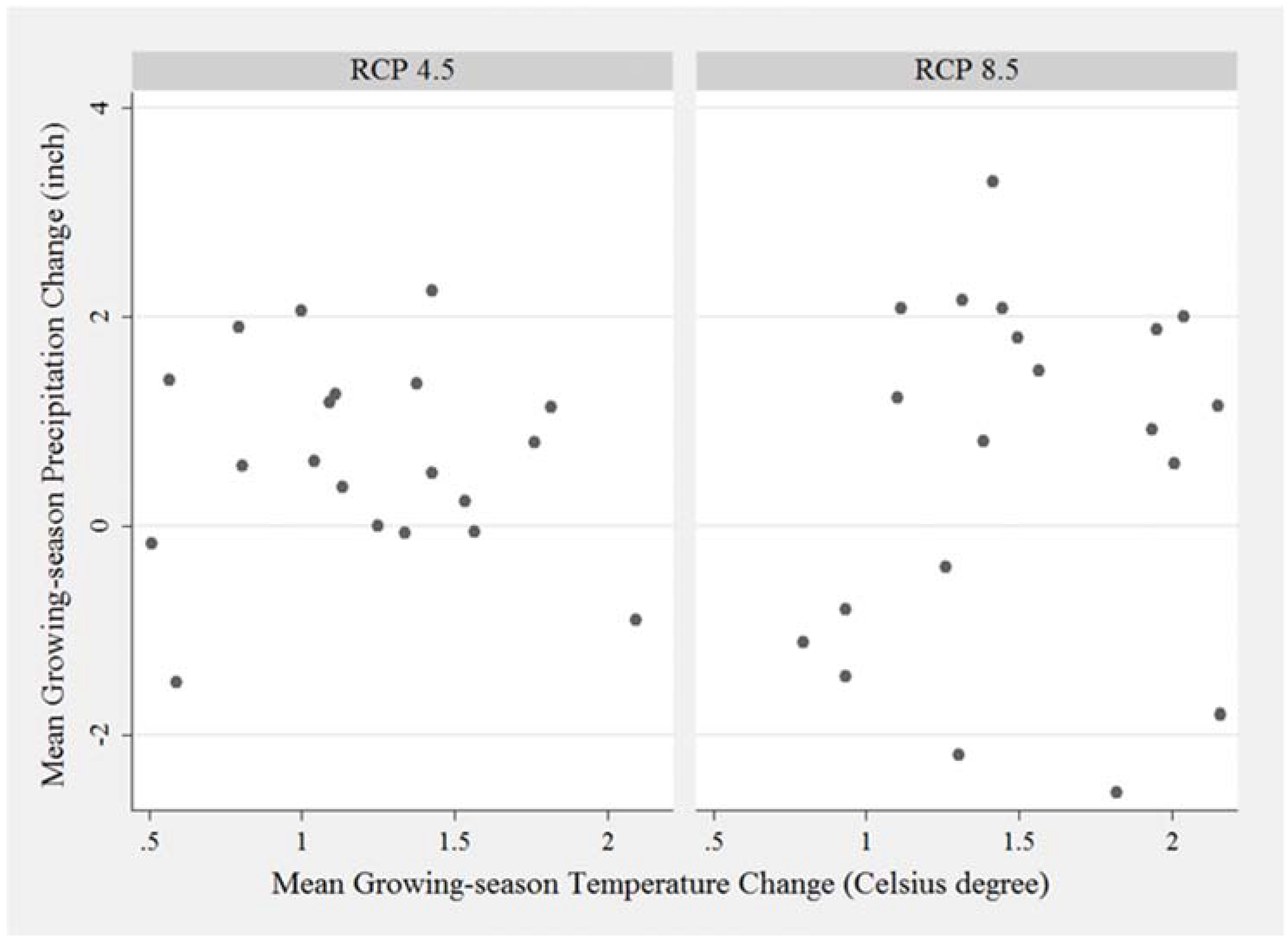
Our projections use two emission scenarios, Representative Concentration Pathways (RCP) 4.5 and 8.5, which represent medium and high greenhouse gas emission levels under moderate and no climate policy. Figure 1 summarizes the projected PNW climate changes arising across the CMIP5 models under RCPs 4.5 and 8.5. Growing season temperature increases across all climate models by 2050 with an average warming of +1.2 °C under RCP 4.5 (intermodel range +0.5 °C to +2.1 °C) and of +1.5 °C under RCP 8.5 (intermodel range +0.8 °C to +2.2 °C). Most climate models project increases in growing season precipitation by 2050, with a multi-model mean increase of +16 mm under RCP 4.5 (intermodel range −38 mm to 57 mm) and of +14 mm under RCP 8.5 (intermodel range –65 mm to 84 mm).
We simulate the share of fallow in total cropland under two climate change scenarios (RCPs 4.5 and 8.5), holding all non-climate variables constant in 2012. The results are summarized in Figure 2. The ensemble projection across all climate models indicates that in wheat farms more land will be fallowed due to a warmer and wetter climate, again showing fallow as an adaptation method. Specifically, on average by 2050, the share of fallowed cropland (1.5 million acres in 2012) will be increased by 1.3% (0.12 million acres) under a medium climate change scenario (RCP 4.5) and by 1.8% (0.16 million acres) under a high climate change scenario (RCP 8.5). Overall, future climate change projections by 2050 are shown to have a small positive effect on fallow acreage in the PNW region, with a large uncertainty arising from global climate models.
5. Conclusions
In this paper, we investigate the relationship between climate and the use of fallow for PNW wheat farms. We find that decreases in growing season precipitation increase the share of fallowed cropland, as do increases in growing season temperature. Using future 2050 climate projections, our simulation results indicate that the share of fallowed cropland will increase by 1.3% and 1.8% under medium and high emission scenarios, respectively, but with substantial uncertainty. These findings suggest that climate causes PNW farmers to put more cropland in fallow, indicating as the climate evolves fallowing is an adaptation strategy.
There are several shortcomings and extensions to this work. First, we only consider the use of fallow, not the changes in types of agricultural land use. With a changing climate, it is likely that some dryland farmers will convert their land to an irrigated use or shift cropland to rangeland or pastureland, while the reverse may also occur. Expanding the study to consider this would be valuable, particularly since land use change is also an observed adaptation strategy [25]. Second, our estimates are a reduced form in the sense that we capture the net effect of the climate on changing cropping systems. Estimating a structural model of a specific crop system is left for future research. Third, our predictions on the share of fallowed cropland are based on current socioeconomic conditions and non-climate biophysical conditions. Future research needs to design scenarios with consistent climate, biophysical and socioeconomic conditions, technologies and policies for projecting changes in fallow acreage [30]. Lastly, our model does not capture the CO2 fertilization effect which has been shown to strongly affect wheat [31] and incorporating this would be desirable.
Acknowledgments
This research was supported in part by USDA-NIFA award #2011-68002-30191.
Author Contributions
Hongliang Zhang and Jianhong E. Mu constructed the initial paper draft, and Bruce A. McCarl improved the organization and presentation to generate the final draft.
Conflicts of Interest
The authors declare no conflict of interest. The funding sponsor had no role in the design of the study; in the collection, analyses, or interpretation of data; in the writing of the manuscript, or in the decision to publish the results.
Appendix A

Table A1.
Estimated coefficients on fallow share for three model specifications.
| Variables | Simple Climate | Add Climate Squared | Add Climate Squared and Variability |
|---|---|---|---|
| Precipitation | −0.37*** | −1.40*** | −1.65*** |
| (0.07) | (0.20) | (0.23) | |
| Average temperature | 0.51** | −1.23 | −0.40 |
| (0.25) | (0.97) | (1.05) | |
| Precipitation square | 0.02*** | 0.01*** | |
| (0.00) | (0.00) | ||
| Average temperature square | 0.13 | 0.06 | |
| (0.08) | (0.09) | ||
| Std. dev. precipitation | 1.64*** | ||
| (0.63) | |||
| Std. dev. average temperature | 1.47 | ||
| (6.29) | |||
| Irrigation proportion | −0.19*** | −0.20*** | −0.20*** |
| (0.01) | (0.01) | (0.01) | |
| CRP and WRP programs | −2.82*** | −3.25*** | −3.43*** |
| (1.03) | (1.10) | (1.14) | |
| Classified as a large farm | −1.02*** | −1.21*** | −1.14*** |
| (0.34) | (0.33) | (0.32) | |
| Years of farming experience | 0.03** | 0.03*** | 0.03** |
| (0.01) | (0.01) | (0.01) | |
| Land tenure | −2.16*** | −2.19*** | −2.23*** |
| (0.38) | (0.37) | (0.37) | |
| Farming occupation | 0.93* | 0.94* | 0.92* |
| (0.49) | (0.49) | (0.49) | |
| Slope | −0.10 | −0.03 | 0.03 |
| (0.06) | (0.06) | (0.06) | |
| Soil organic content | −0.66*** | −0.43** | −0.37* |
| (0.21) | (0.21) | (0.21) | |
| Sand content | −0.44*** | −0.43*** | −0.37*** |
| (0.10) | (0.10) | (0.10) | |
| Silt content | −0.02 | 0.07 | 0.12 |
| (0.11) | (0.11) | (0.11) | |
| Clay content | −0.94*** | −0.91*** | −0.90*** |
| (0.17) | (0.16) | (0.16) | |
| Soil loss tolerance (T) factor | 2.10* | 1.75 | 1.23 |
| (1.17) | (1.14) | (1.16) | |
| Erodibility factor | −37.41*** | −43.18*** | −41.00*** |
| (11.70) | (11.26) | (11.18) | |
| Constant | 59.64*** | 72.79*** | 63.48*** |
| (7.70) | (8.17) | (9.95) | |
| State-year dummy variables | Yes | Yes | Yes |
| Observations | 17,773 | 17,773 | 17,773 |
| R-squared | 0.350 | 0.359 | 0.361 |
Notes: Standard errors are given in parentheses. Coefficient significance is marked with *** p < 0.01, ** p < 0.05, * p < 0.1.
References
- Food and Agriculture Organization of the United Nations. FAOSTAT Statistics Database. Available online: http://www.fao.org/faostat/en/#data (accessed on 27 July 2017).
- Shiferaw, B.; Smale, M.; Braun, H.; Duveiller, E.; Reynolds, M.; Muricho, G. Crops that feed the world 10. Past success and future challenges to the role played by wheat in global food security. Food Secur. 2012, 5, 291–317. [Google Scholar] [CrossRef]
- IPCC. Climate Change 2014: Impacts, Adaptation, and Vulnerability. Part A: Global and Sectoral Aspects. Contribution of Working Group II to the Fifth Assessment Report of the Intergovernmental Panel on Climate Change; Field, C.B., Barros, V.R., Dokken, D.J., Mach, K.J., Mastrandrea, M.D., Bilir, T.E., Chatterjee, M., Ebi, K.L., Estrada, Y.O., Genova, R.C., et al., Eds.; Cambridge University Press: Cambridge, UK; New York, NY, USA, 2014. [Google Scholar]
- Annan, F.; Schlenker, W. Federal crop insurance and the disincentive to adapt to extreme heat. Am. Econ. Rev. Pap. Proc. 2015, 105, 262–266. [Google Scholar] [CrossRef]
- Antle, J.M.; Zhang, H.; Mu, J.; Abatzoglou, J.; Stockle, C. Methods to assess cropping system adaptations to climate change: Dryland wheat systems in the Pacific Northwest United States. Agric. Ecosyst. Environ. 2017, in press. [Google Scholar] [CrossRef]
- Ge, J.; Xu, Y.; Zhong, X.; Li, S.; Tian, S.; Yuan, G.; Cao, C.; Zhan, M.; Zhao, M. Climatic conditions varied by planting date affects maize yield in central China. Agron. J. 2016, 108, 966–977. [Google Scholar] [CrossRef]
- Huang, L.; Sun, Y.; Peng, S.; Wang, F. Genotypic differences of japonica rice responding to high temperature in China. Agron. J. 2016, 108, 626–636. [Google Scholar] [CrossRef]
- McCarl, B.A.; Thayer, A.; Jones, J.P.H. The challenge of climate change adaptation: An economically oriented review. J. Agric. Appl. Econ. 2016, 48, 321–344. [Google Scholar] [CrossRef]
- Mu, J.E.; Antle, J.M.; Abatzoglou, J.T. Climate Change, Weather events, Future Socio-economic Scenarios and Agricultural Land Use; Oregon State University: Corvallis, OR, USA, 2016. [Google Scholar]
- Negri, D.H.; Gollehon, N.R.; Aillery, M.P. The effects of climatic variability on US irrigation adoption. Clim. Chang. 2005, 69, 299–323. [Google Scholar] [CrossRef]
- Ortiz-Bobea, A.; Just, R.E. Modeling the structure of adaptation in climate change impact assessment. Am. J. Agric. Econ. 2013, 95, 244–251. [Google Scholar] [CrossRef]
- Olen, B.; Wu, J.; Langpap, C. Irrigation decisions for major west coast crops: Water scarcity and climatic determinants. Am. J. Agric. Econ. 2016, 98, 254–275. [Google Scholar] [CrossRef]
- Bradshaw, B.; Dolan, H.; Smit, B. Farm–level adaptation to climate variability and change: Crop diversification in the Canadian Prairies. Clim. Chang. 2004, 67, 119–141. [Google Scholar] [CrossRef]
- Howden, S.M.; Soussana, J.; Tubiello, F.N.; Chhetri, N.; Dunlop, M.; Meinke, H. Adapting agricultural to climate change. Proc. Natl. Acad. Sci. USA 2007, 104, 19691–19696. [Google Scholar] [CrossRef] [PubMed]
- Verchot, L.V.; Van Noordwijk, M.; Kandji, S.; Tomich, T.; Ong, C.; Albrecht, A.; Mackensen, J.; Bantilan, C.; Anupama, K.V.; Palm, C. Climate change: Linking adaptation and mitigation through agroforestry. Mitig. Adapt. Strateg. Glob. Chang. 2007, 12. [Google Scholar] [CrossRef]
- Crop Production 2016 Summary; United States Department of Agriculture: Erie, KS, USA, 2017.
- National Agricultural Statistics Service (USDA). Census of Agriculture; National Agricultural Statistics Service (USDA): Helena, MT, USA, 2002.
- Natural Resources Conservation Service (USDA). Gridded Soil Survey Geographic (gSSURGO) Database for the Conterminous United States. Available online: https://gdg.sc.egov.usda.gov/ (accessed on 16 November 2015).
- Abatzoglou, J.T. Development of gridded surface meteorological data for ecological applications and modelling. Int. J. Climatol. 2011. [Google Scholar] [CrossRef]
- Abatzoglou, J.T.; Brown, T.J. A comparison of statistical downscaling methods suited for wildfire applications. Int. J. Climatol. 2012, 32, 772–780. [Google Scholar] [CrossRef]
- Adams, R.M. Global Climate Change and Agriculture: An Economic Perspective. Am. J. Agric. Econ. 1989, 71, 1272–1279. [Google Scholar] [CrossRef]
- Mendelsohn, R.; Nordhaus, W.D.; Shaw, D. The impact of global warming on agriculture: A Ricardian analysis. Am. Econ. Rev. 1994, 84, 753–771. [Google Scholar]
- McCarl, B.A.; Villavicencio, X.; Wu, X.M. Climate change and future analysis: Is stationarity dying? Am. J. Agric. Econ. 2008, 90, 1242–1247. [Google Scholar] [CrossRef]
- Schlenker, W.; Roberts, M.J. Nonlinear temperature effects indicate severe damage to U.S. crop yields under climate change. Proc. Natl. Acad. Sci. USA 2009, 106, 15594–15598. [Google Scholar] [CrossRef] [PubMed]
- Mu, J.E.; McCarl, B.A.; Wein, A.M. Adaptation to climate change: Changes in farmland use and stocking rate in the U.S. Mitig. Adapt. Strateg. Glob. Chang. 2013, 18, 713–730. [Google Scholar] [CrossRef]
- Jiang, P.; Thelen, K.D. Effect of soil and topographic properties on crop yield in a North–Central corn–soybean cropping system. Agron. J. 2004, 96, 252–258. [Google Scholar] [CrossRef]
- Stewart, C.M.; McBratney, A.B.; Skerritt, J.H. Site–specific durum wheat quality and its relationship to soil properties in a single field in Northern New South Wales. Precis. Agric. 2002, 3, 155–168. [Google Scholar] [CrossRef]
- Deschenes, O.; Greenstone, M. The economic impacts of climate change: evidence from agricultural output and random fluctuations in weather. Am. Econ. Rev. 2007, 97, 354–385. [Google Scholar] [CrossRef]
- Flato, G.; Marotzke, J.; Abiodun, B.; Braconnot, P.; Chou, S.C.; Collins, W.; Cox, P.; Driouech, F.; Emori, S.; Eyring, V.; et al. Evaluation of climate models. In Climate Change 2007: The Physical Science Basis. Contribution of Working Group I to the Fourth Assessment Report of the Intergovernmental Panel on Climate Change; Stocker, T.F., Qin, D., Plattner, G.-K., Tignor, M., Allen, S.K., Boschung, J., Nauels, A., Xia, Y., Bex, V., Midgley, P.M., Eds.; Cambridge University Press: Cambridge, UK; New York, NY, USA, 2013; pp. 741–866. [Google Scholar]
- Mu, J.E.; Sleeter, B.; Abatzoglou, J.; Antle, J. Climate impacts on agricultural land use in the United States: the role of socio–economic scenarios. Clim. Chang. 2007. Available online: http://link.springer.com/article/10.1007/s10584-017-2033-x (accessed on 11 August 2017).
- Attavanich, W.; McCarl, B.A. How is CO2 affecting yields and technological progress? A statistical analysis. Clim. Chang. 2014, 124, 747–762. [Google Scholar] [CrossRef]
Figure 1.
Projected changes in mean growing season total precipitation and average temperature by 2050 with a baseline period from 1982–2011. Each dot represents a projection from a particular CMIP5 climate model.
Figure 1.
Projected changes in mean growing season total precipitation and average temperature by 2050 with a baseline period from 1982–2011. Each dot represents a projection from a particular CMIP5 climate model.

Figure 2.
Projected change in fallow share for wheat farms in the PNW region by 2050 (Unit: %).
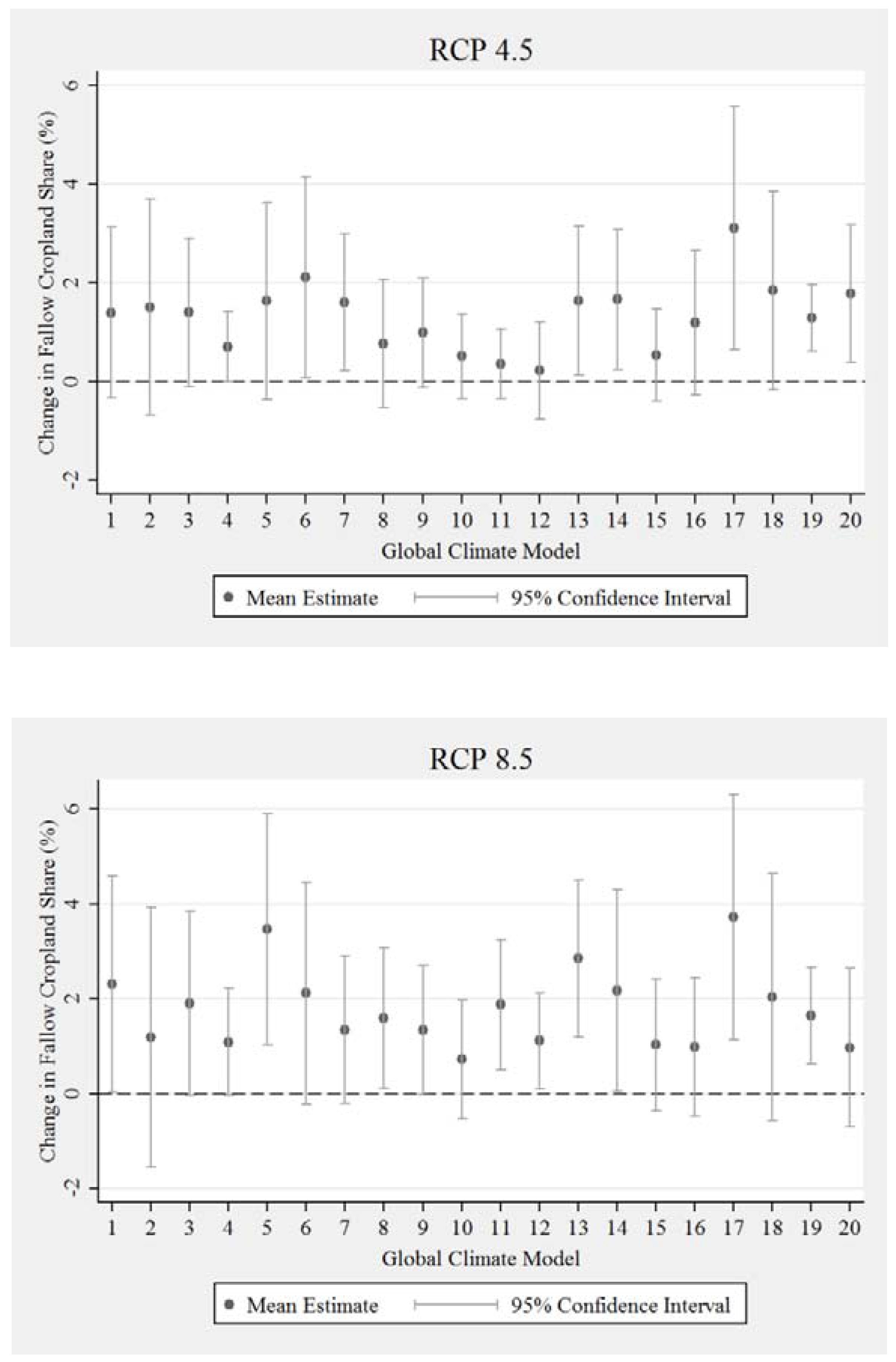
Table 1.
Summary of statistics of wheat farms in the Pacific Northwest region from the U.S. Census of Agriculture.
Table 1.
Summary of statistics of wheat farms in the Pacific Northwest region from the U.S. Census of Agriculture.
| All Farms | Farms That Did Not Fallow | Farms That Did Fallow | Variable Description | ||||
|---|---|---|---|---|---|---|---|
| Mean | Std. Dev. | Mean | Std. Dev. | Mean | Std. Dev. | ||
| Panel A | |||||||
| Fallow proportion | 11.20 | 17.87 | 0.00 | 0.00 | 29.53 | 17.34 | Share of fallowed cropland in percent |
| Irrigation proportion | 0.39 | 0.48 | 0.55 | 0.49 | 0.12 | 0.30 | Percent of irrigated wheat acreage |
| CRP and WRP programs | 0.06 | 0.21 | 0.04 | 0.22 | 0.09 | 0.18 | Share of cropland under CRP and WRP programs |
| Classified as a large farm | 0.61 | 0.49 | 0.61 | 0.49 | 0.60 | 0.49 | Annual farm revenue of over $250,000 (1 = yes, 0 = no) |
| Years of farming experience | 25.86 | 13.68 | 25.50 | 13.65 | 26.44 | 13.73 | Farming experience (years) |
| Land tenure | 0.82 | 0.38 | 0.85 | 0.36 | 0.78 | 0.41 | Farmland fully or partially owned by an operator (1 = yes, 0 = no) |
| Farming occupation | 0.90 | 0.30 | 0.89 | 0.31 | 0.91 | 0.29 | Operator occupation (1 = farming, 0 = employed off-farm) |
| Panel B | |||||||
| Slope | 14.00 | 8.62 | 12.63 | 8.79 | 16.23 | 7.84 | Average land slope in percent |
| Soil organic content | 7.88 | 4.41 | 7.90 | 4.79 | 7.85 | 3.69 | Soil organic matter in 1 meter depth (kg C/m2) |
| Sand content | 27.27 | 12.18 | 28.37 | 12.69 | 25.47 | 11.06 | Percent of particles with 0.05–2 mm in diameter |
| Silt content | 45.32 | 11.46 | 44.08 | 11.45 | 47.35 | 11.20 | Percent of particles with 0.002–0.05 mm in diameter |
| Clay content | 15.27 | 5.85 | 15.78 | 6.05 | 14.44 | 5.42 | Percent of particles with <0.002 mm in diameter |
| Soil loss tolerance (T) factor | 3.65 | 0.72 | 3.63 | 0.72 | 3.69 | 0.72 | Soil loss tolerance factor (tons/acre/year) |
| Erodibility factor | 0.37 | 0.09 | 0.36 | 0.09 | 0.37 | 0.09 | Soil erodibility factor (value range from 0.02–0.68) |
| Panel C | |||||||
| Precipitation | 16.22 | 9.75 | 16.75 | 11.05 | 15.35 | 7.05 | 22-year average of growing season total precipitation (inch) |
| Average temperature | 7.09 | 1.74 | 7.09 | 1.87 | 7.09 | 1.49 | 22-year average of growing season average temperature (°C) |
| Std. dev. precipitation | 3.61 | 2.11 | 3.83 | 2.38 | 3.24 | 1.49 | Standard deviation of growing season total precipitation (inch) |
| Std. dev. average temp. | 0.77 | 0.11 | 0.77 | 0.12 | 0.77 | 0.10 | Standard deviation of growing season average temperature (°C) |
| Maximum temperature | 13.16 | 1.54 | 13.27 | 1.64 | 12.99 | 1.36 | 22-year average of growing season maximum temperature (°C) |
| Std. dev. maximum temp. | 0.94 | 0.12 | 0.95 | 0.13 | 0.92 | 0.09 | Standard deviation of growing season maximum temperature (°C) |
| Growing degree-days | 23.82 | 3.79 | 23.92 | 4.04 | 23.65 | 3.34 | 22-year average of growing degree-days (100 degree-days) |
| Freezing degree-days | 2.38 | 1.67 | 2.50 | 1.84 | 2.20 | 1.34 | 22-year average of freezing degree-days (100 degree-days) |
| Std. dev. GDD | 1.52 | 0.15 | 1.52 | 0.17 | 1.52 | 0.13 | Standard deviation of growing degree-days (100 degree-days) |
| Std. dev. FDD | 1.12 | 0.47 | 1.13 | 0.52 | 1.10 | 0.37 | Standard deviation of freezing degree-days (100 degree-days) |
| Sample size | 17,773 | 11,033 | 6740 | ||||
Notes: All climate variables in Panel C are computed over the winter wheat growing season from September to June (inclusive).
Table 2.
Estimated marginal effects on fallow share for three model specifications (Unit: %).
| Variables | Simple Climate | Climate Squared | Climate Squared and Variability |
|---|---|---|---|
| Precipitation | −0.37*** | −0.88*** | −1.18*** |
| (0.07) | (0.11) | (0.17) | |
| Average temperature | 0.51** | 0.60** | 0.50 |
| (0.25) | (0.30) | (0.31) | |
| Std. dev. precipitation | 1.64*** | ||
| (0.63) | |||
| Std. dev. average temperature | 1.47 | ||
| (0.063) | |||
| Irrigation proportion | −0.19*** | −0.20*** | −0.20*** |
| (0.01) | (0.01) | (0.01) | |
| CRP and WRP programs | −2.82*** | −3.25*** | −3.43*** |
| (1.03) | (1.10) | (1.14) | |
| Classified as a large farm | −1.02*** | −1.21*** | −1.14*** |
| (0.34) | (0.33) | (0.32) | |
| Years of farming experience | 0.03** | 0.03*** | 0.03** |
| (0.01) | (0.01) | (0.01) | |
| Land tenure | −2.16*** | −2.19*** | −2.23*** |
| (0.38) | (0.37) | (0.37) | |
| Farming occupation | 0.93* | 0.94* | 0.92* |
| (0.49) | (0.49) | (0.49) | |
| Slope | −0.10 | −0.03 | 0.03 |
| (0.06) | (0.06) | (0.06) | |
| Soil organic content | −0.66*** | −0.43** | −0.37* |
| (0.21) | (0.21) | (0.21) | |
| Sand content | −0.44*** | −0.43*** | −0.37*** |
| (0.10) | (0.10) | (0.10) | |
| Silt content | -0.02 | 0.07 | 0.12 |
| (0.11) | (0.11) | (0.11) | |
| Clay content | −0.94*** | −0.91*** | −0.90*** |
| (0.17) | (0.16) | (0.16) | |
| Soil loss tolerance (T) factor | 2.10* | 1.75 | 1.23 |
| (1.17) | (1.14) | (1.16) | |
| Erodibility factor | −37.41*** | −43.18*** | −41.00*** |
| (11.70) | (11.26) | (11.18) | |
| Intercept | Yes | Yes | Yes |
| State-year dummy variables | Yes | Yes | Yes |
| R-squared | 0.350 | 0.359 | 0.361 |
| Observations | 17,773 | 17,773 | 17,773 |
Notes: We estimate three versions of the linear probability model using different combinations of climate variables. The three sets of climate variables are: (1) the simple climate model with the 22-year averaged growing season precipitation and average temperature; (2) the same variables in the simple climate model and squared terms of the climate variables and (3) the linear and squared climate variables and standard deviations of precipitation and temperature. Standard errors are given in parentheses. Coefficient significance is marked with *** p < 0.01, ** p < 0.05, * p < 0.1.
Table 3.
Estimated marginal effects of climate on fallow share for robustness checks (Unit: %).
| Variables | Using Maximum Temperature | Using Growing and Freezing Degree-days |
|---|---|---|
| Precipitation | −1.29*** | −1.08*** |
| (0.17) | (0.19) | |
| Std. dev. precipitation | 2.04*** | 1.38* |
| (0.61) | (0.71) | |
| Maximum temperature | 0.10 | |
| (0.33) | ||
| Std. dev. maximum temperature | −15.77*** | |
| (4.82) | ||
| Growing degree-days | 0.56* | |
| (0.31) | ||
| Freezing degree-days | 1.47 | |
| (1.60) | ||
| Std. dev. growing degree-days | −3.71 | |
| (3.66) | ||
| Std. dev. freezing degree-days | −2.14 | |
| (2.88) |
Notes: We re-estimate two versions of the climate squared and variability model in Table 2 by using different temperature variables for robustness check: (1) 22-year average and standard deviation of growing season maximum temperature –using maximum temperature; (2) 22-year averages and standard deviations of growing degree-days and freezing degree-days –using growing and freezing degree-days. Precipitation, soil and socioeconomic variables are the same as in the third model in Table 2. Standard errors are in parentheses with significance levels marked as *** p < 0.01, ** p < 0.05, * p < 0.1.
© 2017 by the authors. Licensee MDPI, Basel, Switzerland. This article is an open access article distributed under the terms and conditions of the Creative Commons Attribution (CC BY) license (http://creativecommons.org/licenses/by/4.0/).
Share and Cite
MDPI and ACS Style
Zhang, H.; Mu, J.E.; McCarl, B.A. Adaption to Climate Change through Fallow Rotation in the U.S. Pacific Northwest. Climate 2017, 5, 64. https://doi.org/10.3390/cli5030064
AMA Style
Zhang H, Mu JE, McCarl BA. Adaption to Climate Change through Fallow Rotation in the U.S. Pacific Northwest. Climate. 2017; 5(3):64. https://doi.org/10.3390/cli5030064
Chicago/Turabian StyleZhang, Hongliang, Jianhong E. Mu, and Bruce A. McCarl. 2017. "Adaption to Climate Change through Fallow Rotation in the U.S. Pacific Northwest" Climate 5, no. 3: 64. https://doi.org/10.3390/cli5030064
Note that from the first issue of 2016, this journal uses article numbers instead of page numbers. See further details here.