
Performance Assessment of Multi-Source Weighted-Ensemble Precipitation (MSWEP) Product over India

Abstract
:
1. Introduction
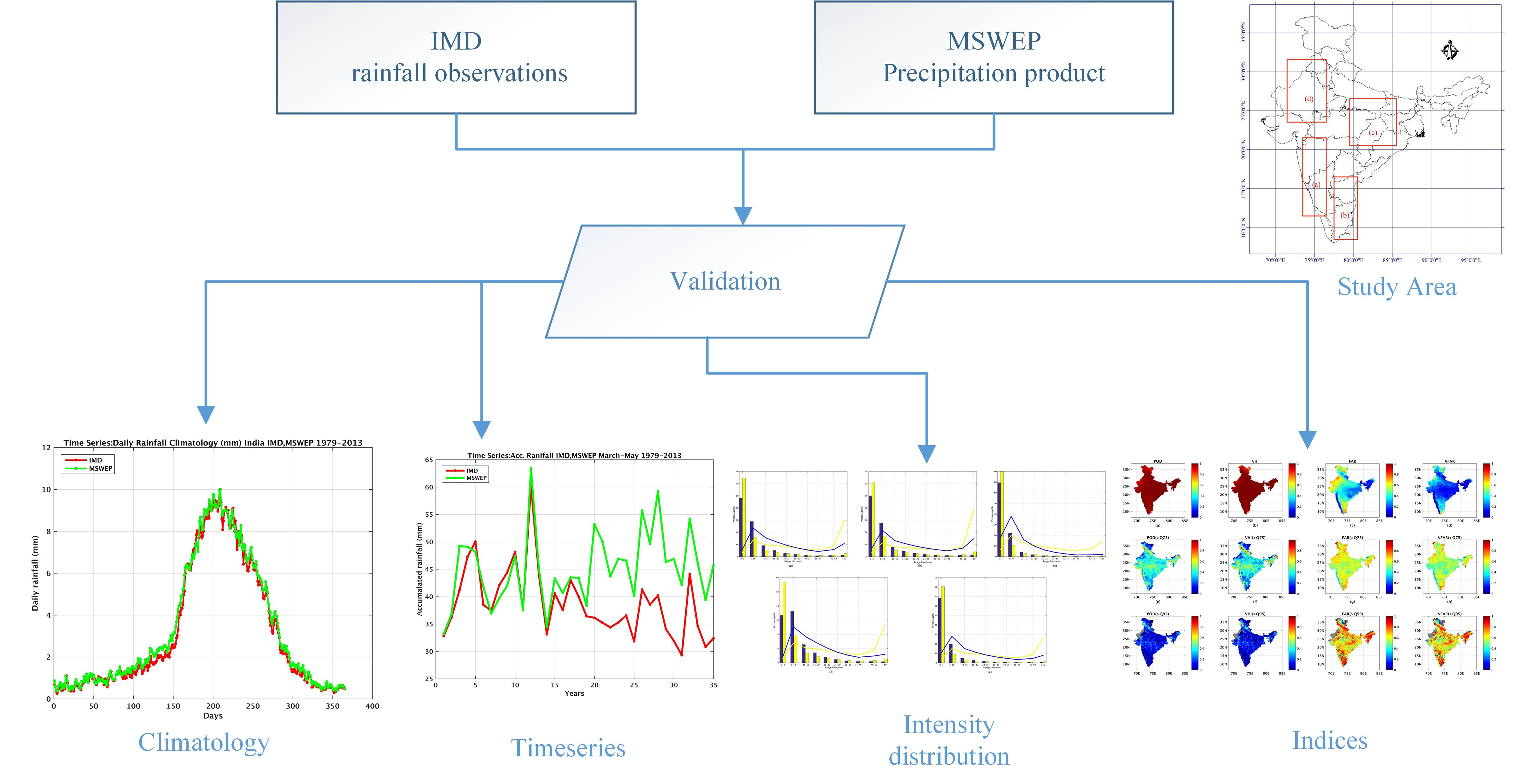
2. Data Used
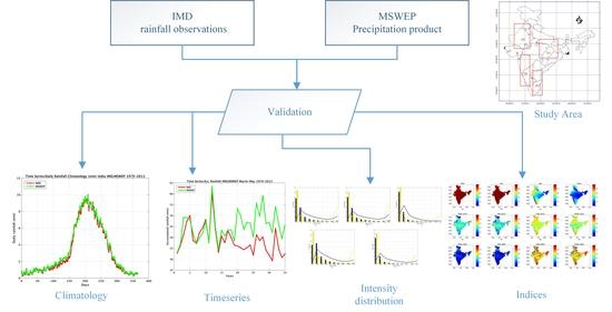
3. Methodology
4. Results
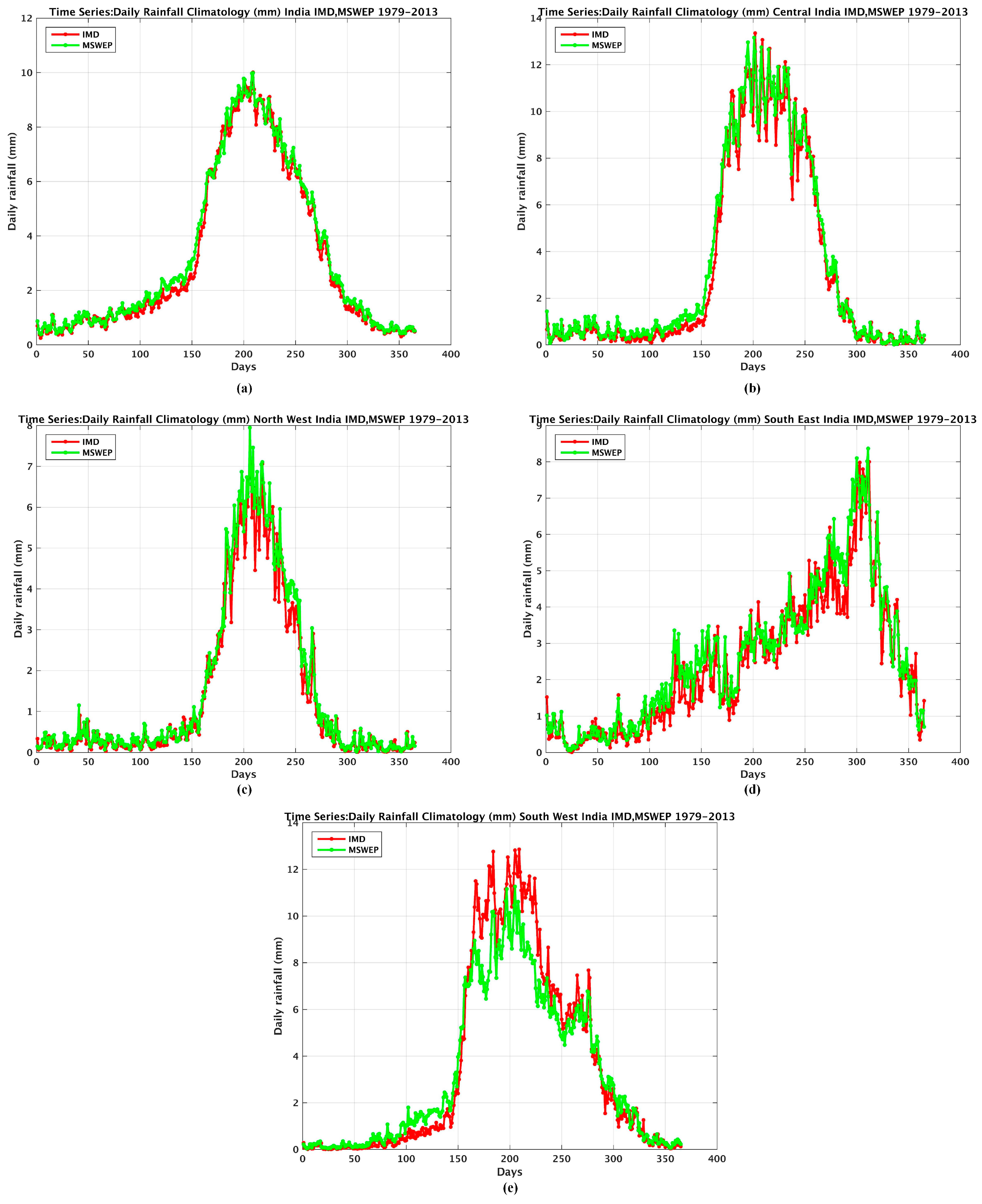
4.1. Rainfall Climatology
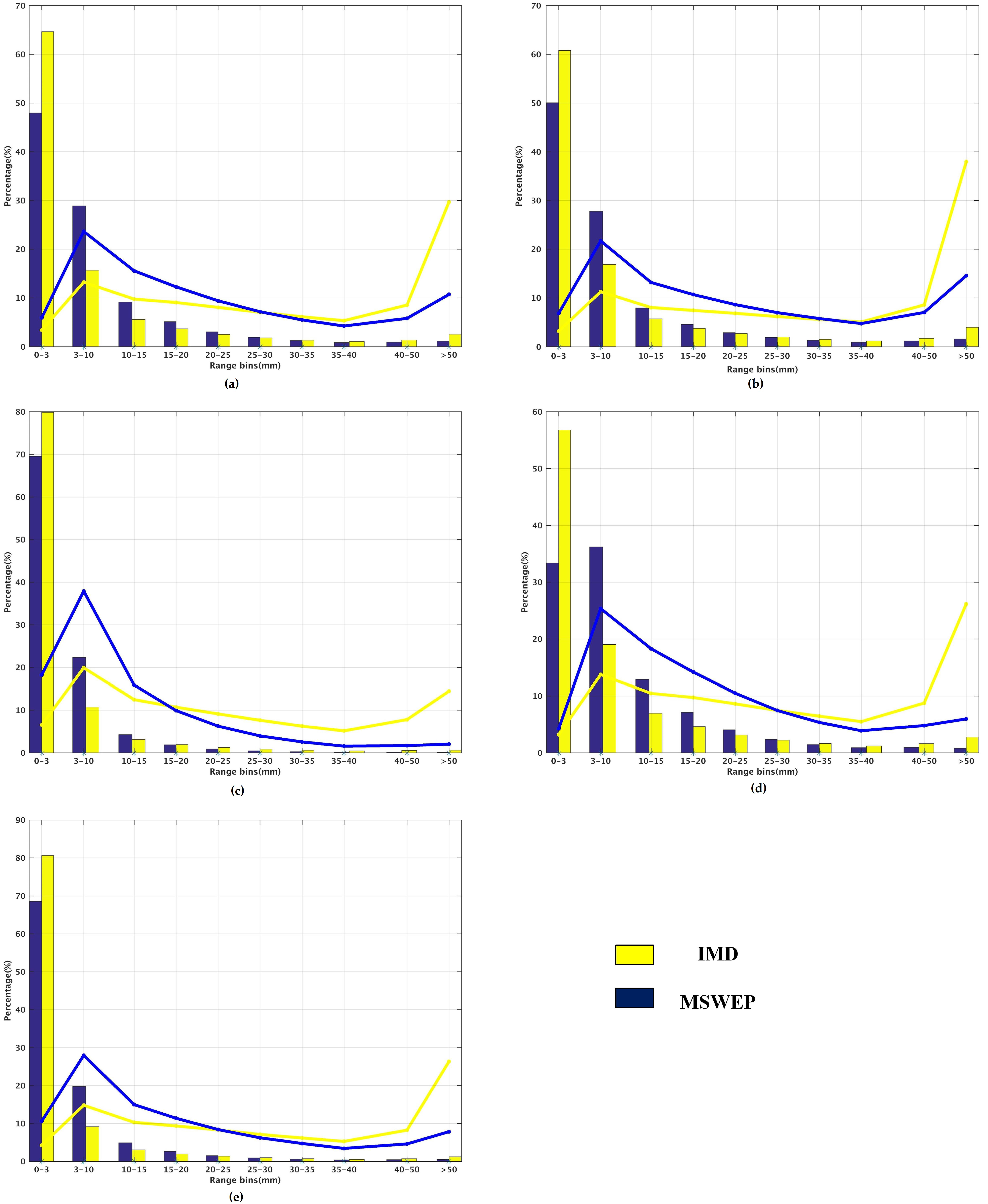
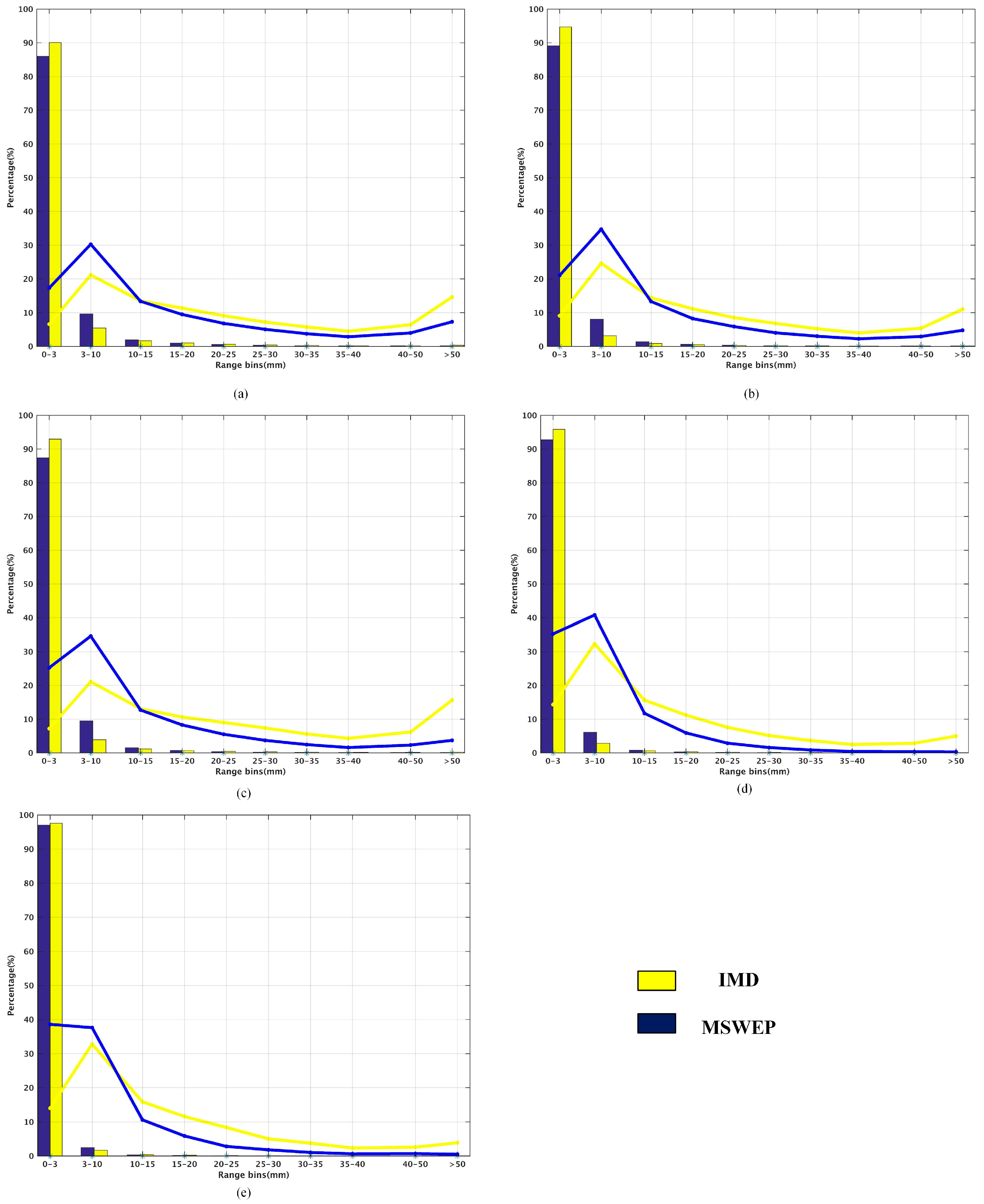
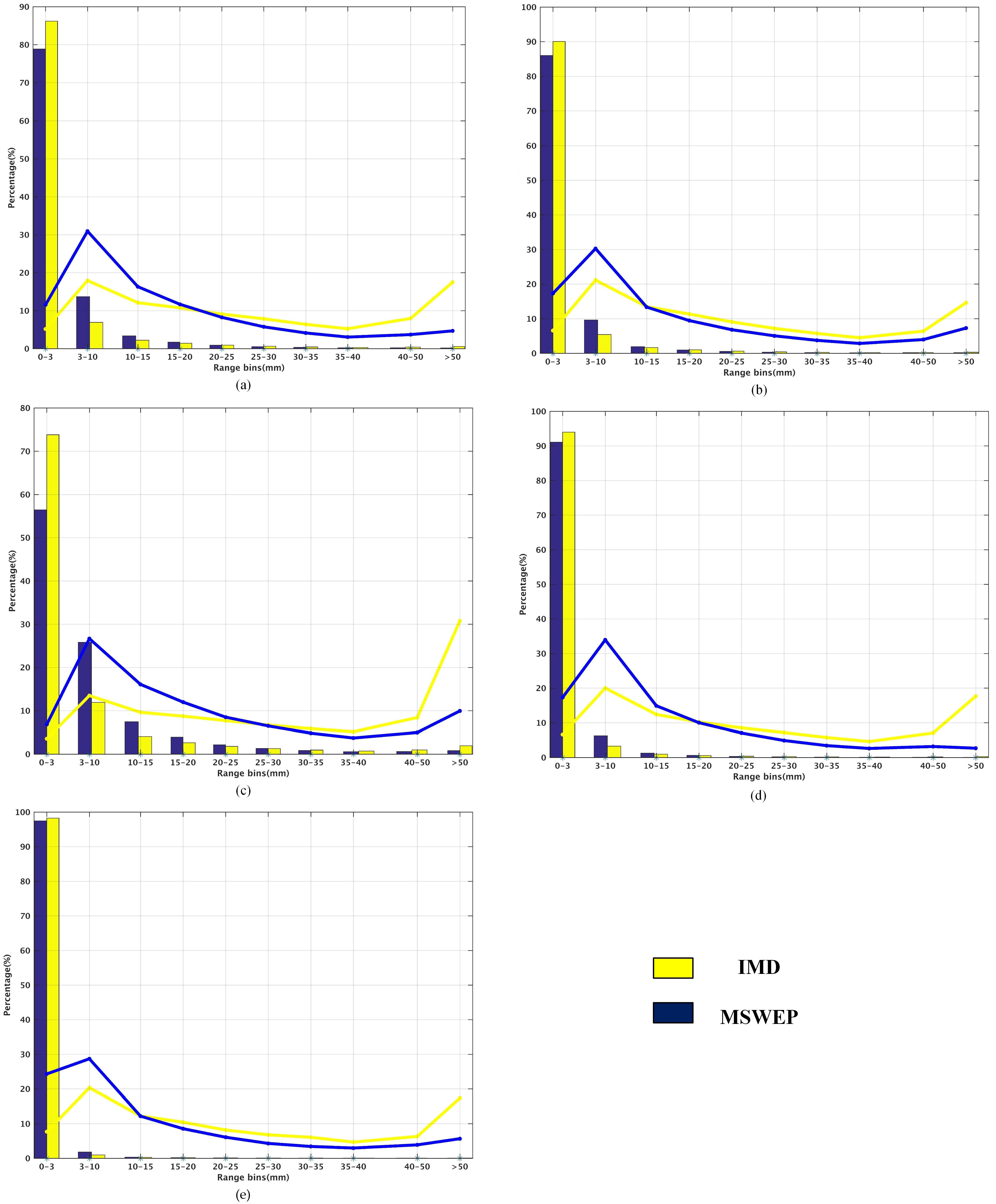
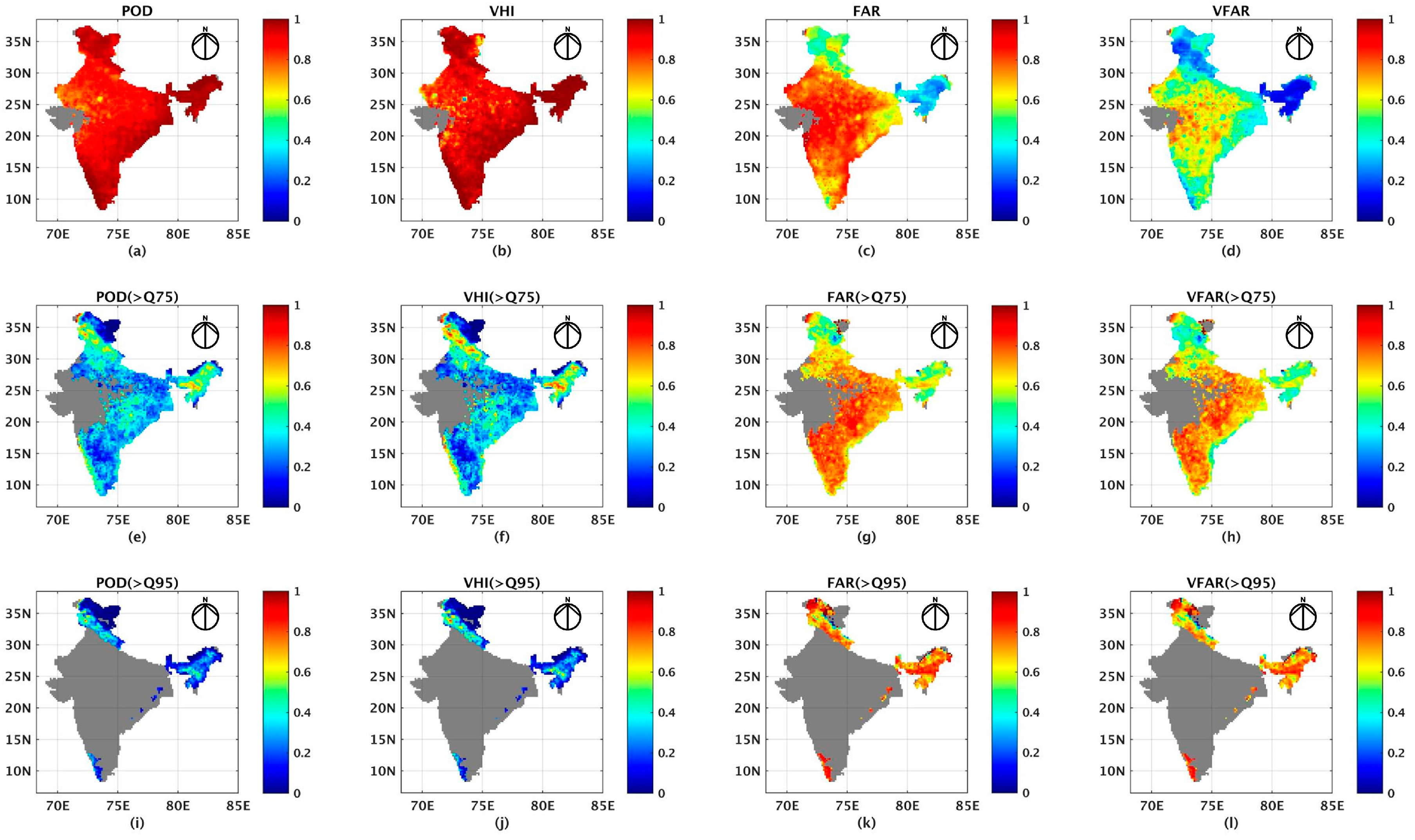
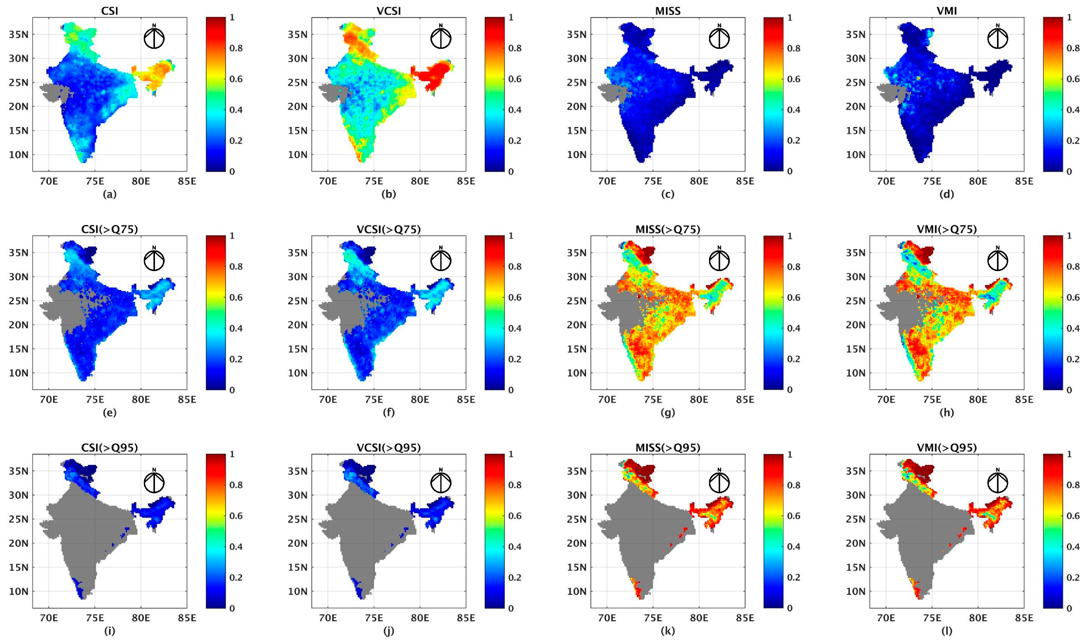
4.2. Evaluation of the Rainfall Data under Different Rainfall Intensity
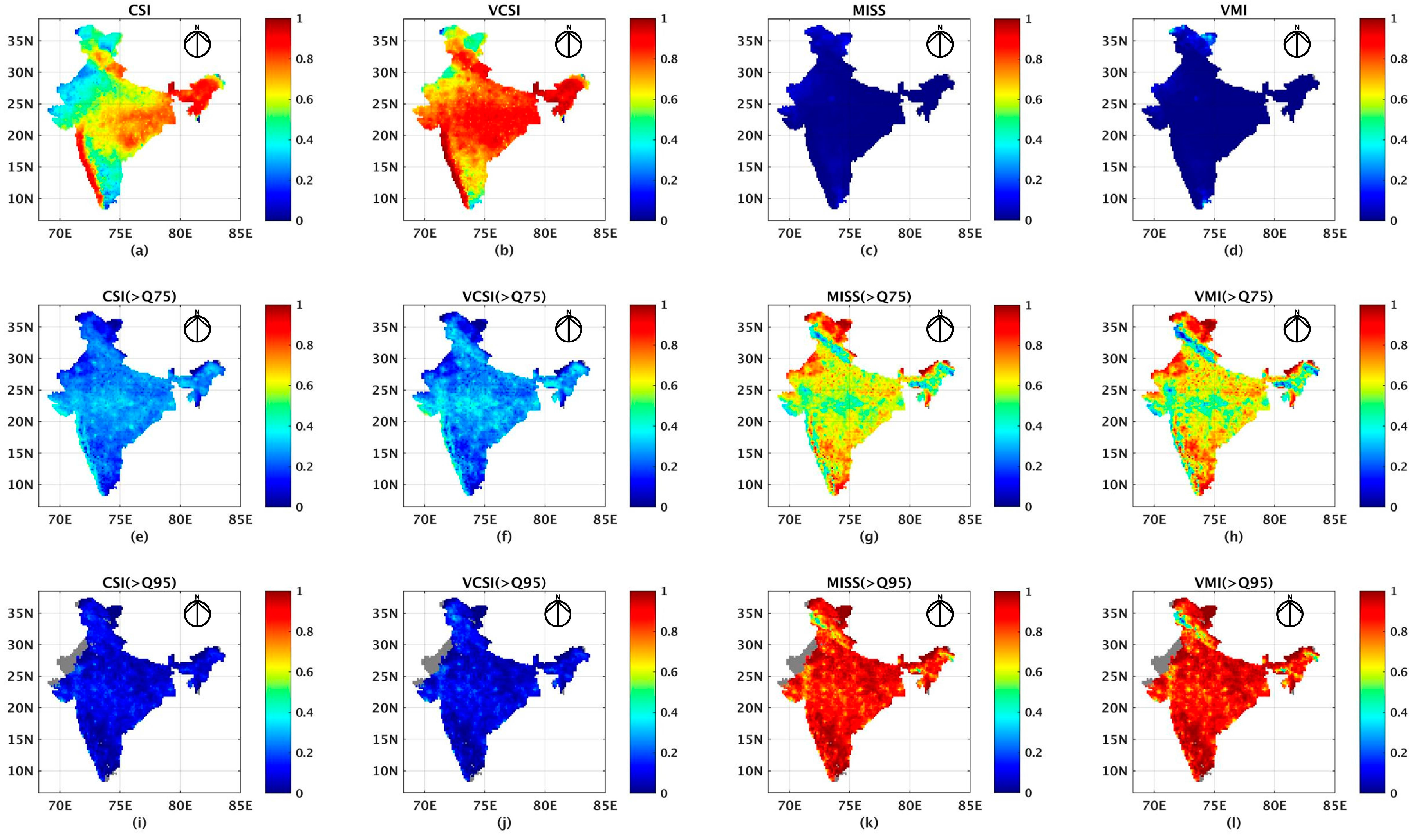
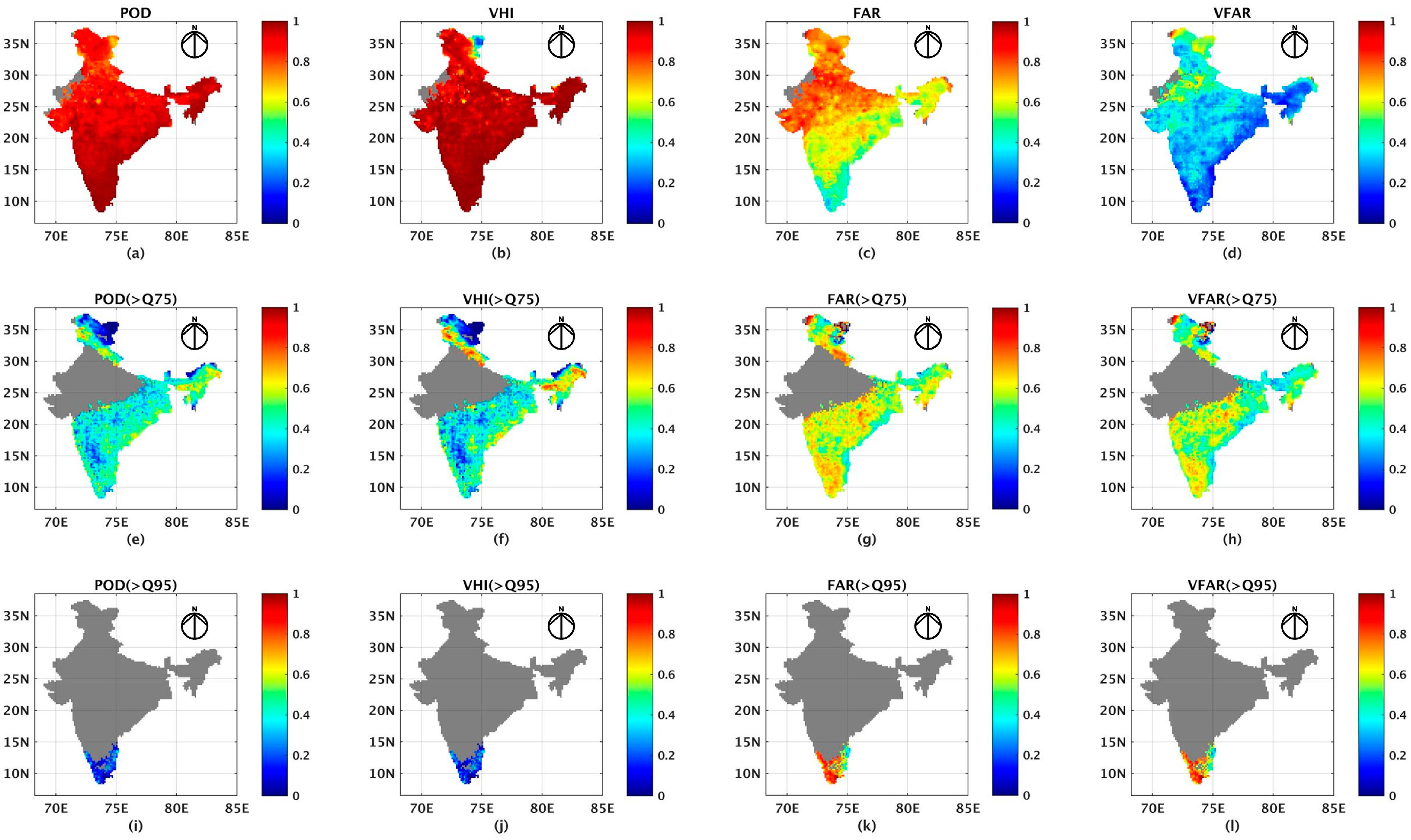
4.3. Results for the Monsoon Season
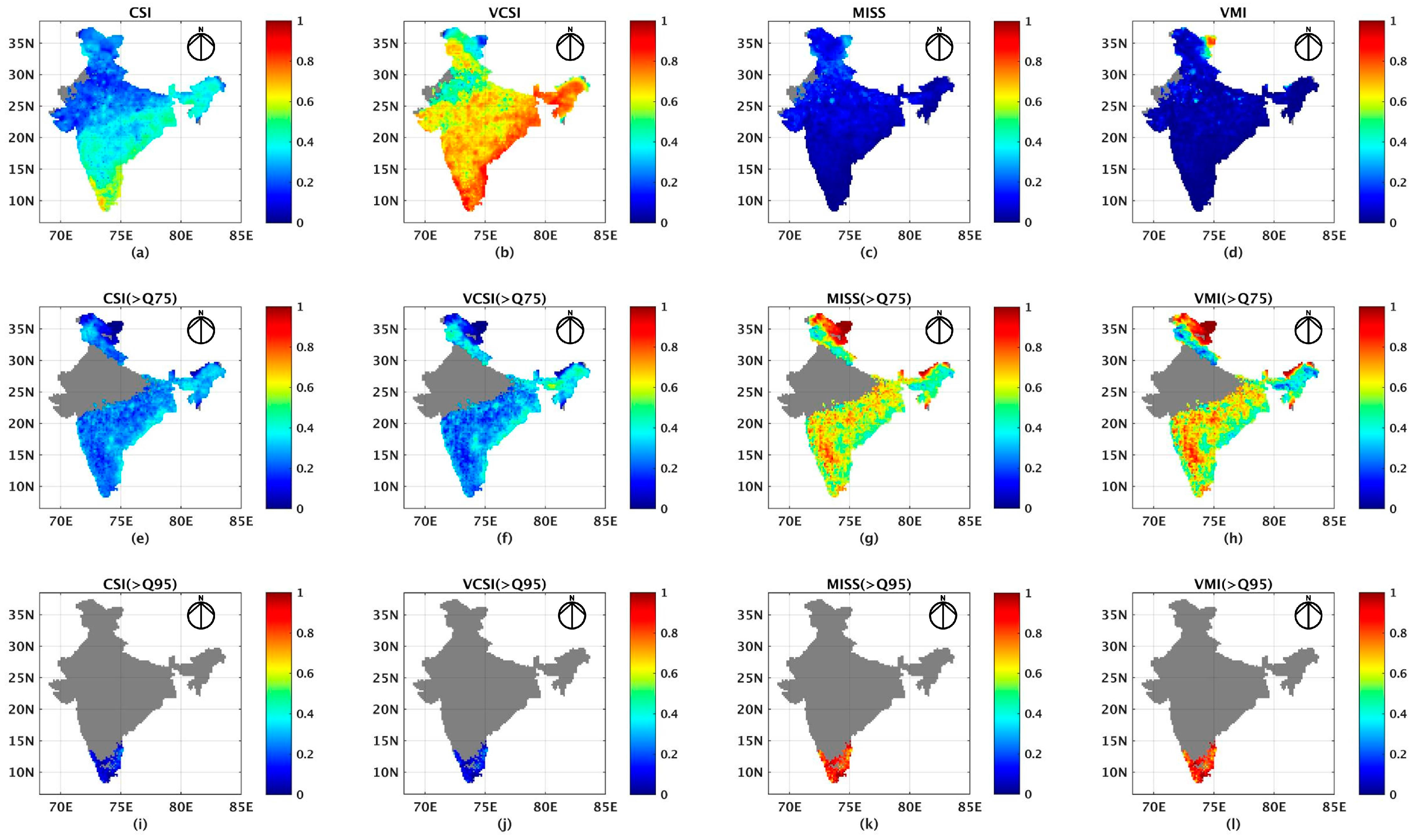
4.4. Comparison for the Post-Monsoon Season
4.5. Comparative Analysis for the Pre-Monsoon Season
5. Conclusions
Acknowledgments
Author Contributions
Conflicts of Interest
References
- Ebert, E.; Janowiak, J.; Kidd, C. Comparison of near-real-time precipitation estimates from satellite observations and numerical models. Bull. Am. Meteorol. Soc. 2007, 88, 47–64. [Google Scholar] [CrossRef]
- Huffman, G.J.; Adler, R.F.; Bolvin, D.T.; Gu, G.J.; Nelkin, E.J.; Bowman, K.P.; Hong, Y.; Stocker, E.F.; Wolff, D.B. The TRMM multisatellite precipitation analysis (TMPA): Quasi-global, multiyear, combined-sensor precipitation estimates at fine scales. J. Hydrometeorol. 2007, 8, 38–55. [Google Scholar] [CrossRef]
- Huffman, G.J.; Adler, R.F.; Bolvin, D.T.; Nelkin, E.J. The TRMM multi-satellite precipitation analysis (TMPA). In Satellite Rainfall Applications for Surface Hydrology; Springer: Dordrecht, The Netherlands, 2010; pp. 3–22. [Google Scholar]
- Huffman, G.J.; Bolvin, D.T.; Nelkin, E.J. Integrated Multi-Satellite Retrievals for GPM (IMERG) Technical Documentation; NASA/GSFC: Greenbelt, MD, USA, 2014.
- Joyce, R.J.; Janowiak, J.E.; Arkin, P.A.; Xie, P. CMORPH: A method that produces global precipitation estimates from passive microwave and infrared data at high spatial and temporal resolution. J. Hydrometeorol. 2004, 5, 487–503. [Google Scholar] [CrossRef]
- Xie, P.; Chen, M.; Shi, W. CPC unified gauge-based analysis of global daily precipitation. In Proceedings of the 24th Conference on Hydrology, Atlanta, GA, USA, 18 January 2010.
- Kubota, T.; Shige, S.; Hashizume, H.; Aonashi, K.; Takahashi, N.; Seto, S.; Hirose, M.; Takayabu, Y.N.; Ushio, T.; Nakagawa, K.; et al. Global precipitation map using satellite-borne microwave radiometers by the GSMaP project: Production and validation. IEEE Trans. Geosci. Remote Sens. 2007, 45, 2259–2275. [Google Scholar] [CrossRef]
- Ushio, T.; Tashima, T.; Kubota, T.; Kachi, M. Gauge adjusted global satellite mapping of precipitation (GSMaP_Gauge). In Proceedings of the 29th ISTS (International Symposium on Space Technology and Science), Nagoya-Aichi, Japan, 2–9 June 2013.
- Huffman, G.J.; Adler, R.F.; Arkin, P.; Chang, A.; Ferraro, R.; Gruber, A.; Janowiak, J.; McNab, A.; Rudolf, B.; Schneider, U. The global precipitation climatology project (GPCP) combined precipitation dataset. Bull. Am. Meteorol. Soc. 1997, 78, 5–20. [Google Scholar] [CrossRef]
- Morrissey, M.; Greene, J. Uncertainty analysis of satellite rainfall algorithms over the tropical Pacific. J. Geophys. Res. Atmos. 1998, 103, 19569–19576. [Google Scholar] [CrossRef]
- McPhee, J.; Margulis, S.A. Validation and error characterization of the GPCP-1DD precipitation product over the contiguous United States. J. Hydrometeorol. 2005, 6, 441–459. [Google Scholar] [CrossRef]
- Tian, Y.; Peters-Lidard, C.; Eylander, J.; Joyce, R.; Huffman, G.; Adler, R.; Hsu, K.; Turk, F.; Garcia, M.; Zeng, J. Component analysis of errors in satellite-based precipitation estimates. J. Geophys. Res. 2009, 114, D24101. [Google Scholar] [CrossRef]
- Habib, E.; Henschke, A.; Adler, R.F. Evaluation of TMPA satellite-based research and rea-time rainfall estimates during six tropical related heavy rainfall events over Louisiana, USA. Atmos. Res. 2009, 94, 373–388. [Google Scholar] [CrossRef]
- Sapiano, M.R.P.; Arkin, P.A. An intercomparison and validation of high-resolution satellite precipitation estimates with 3-hourly gauge data. J. Hydrometeorol. 2009, 10, 149–166. [Google Scholar] [CrossRef]
- Tian, Y.; Peters-Lidard, C.D. A global map of uncertainties in satellite-based precipitation measurements. Geophys. Res. Lett. 2010, 37. [Google Scholar] [CrossRef]
- Shen, Y.; Xiong, A.Y.; Wang, Y.; Xie, P.P. Performance of high-resolution satellite precipitation products over China. J. Geophys. Res. Atmos. 2010, 115. [Google Scholar] [CrossRef]
- Anagnostou, E.N.; Maggioni, V.; Nikolopoulos, E.I.; Meskele, T.; Hossain, F.; Papadopoulos, A. Benchmarking high-resolution global satellite rainfall products to radar and rain-gauge rainfall estimates. IEEE Trans. Geosci. Remote Sens. 2010, 48, 1667–1683. [Google Scholar] [CrossRef]
- Stampoulis, D.; Anagnostou, E.N. Evaluation of global satellite rainfall products over continental Europe. J. Hydrometeorol. 2012, 13, 588–603. [Google Scholar] [CrossRef]
- Habib, E.; Haile, A.T.; Tian, Y.; Joyce, R.J. Evaluation of the high-resolution CMORPH satellite rainfall product using dense rain gauge observations and radar-based estimates. J. Hydrometeorol. 2012, 13, 1784–1798. [Google Scholar] [CrossRef]
- Kisrtetter, P.E.; Viltard, N.; Gosset, M. An error model for instantaneous satellite rainfall estimates: Evaluation of BRAIN-TMI over West Africa. Q. J. R. Meteorol. Soc. 2012, 139, 894–911. [Google Scholar]
- Chen, S.; Hong, Y.; Gourley, J.J.; Huffman, G.J.; Tian, Y.; Cao, Q.; Yong, B.; Kirstetter, P.E.; Hu, J.; Hardy, J. Evaluation of the successive V6 and V7 TRMM multisatellite precipitation analysis over the Continental United States. Water Resour. Res. 2013, 49, 8174–8186. [Google Scholar] [CrossRef]
- Joshi, M.K.; Rai, A.; Pandey, A.C. Validation of TMPA and GPCP 1DD against the ground truth rain-gauge data for Indian region. Int. J. Climatol. 2013, 33, 2633–2648. [Google Scholar] [CrossRef]
- Nair, S.; Srinivasan, G.; Nemani, R. Evaluation of multi-satellite TRMM derived rainfall estimates over a western state of India. J. Meteorol. Soc. Jpn. 2009, 87, 927–939. [Google Scholar] [CrossRef]
- Prakash, S.; Sathiyamoorthy, V.; Mahesh, C.; Gairola, R.M. An evaluation of high-resolution multisatellite rainfall products over the Indian monsoon region. Int. J. Remote Sens. 2014, 35, 3018–3035. [Google Scholar] [CrossRef]
- Prakash, S.; Mitra, A.K.; Rajagopal, E.N.; Pai, D.S. Assessment of TRMM-based TMPA-3B42 and GSMaP precipitation products over India for the peak southwest monsoon season. Int. J. Climatol. 2015, 36, 1614–1631. [Google Scholar] [CrossRef]
- Indu, J.; Kumar, D.N. Evaluation of precipitation retrievals from orbital data products of TRMM over a subtropical basin in India. IEEE Trans. Geosci. Remote Sens. 2015, 53, 6429–6442. [Google Scholar] [CrossRef]
- Alemohammad, S.H.; McLaughlin, D.B.; Entekhabi, E. Quantifying precipitation uncertainty for land data assimilation applications. Mon. Weather Rev. 2015, 143, 3276–3299. [Google Scholar] [CrossRef]
- AghaKouchak, A.; Bardossy, A.; Habib, E. Copula-based uncertainty modelling: application to multisensory precipitation estimates. Hydrol. Process. 2010, 24, 2111–2124. [Google Scholar] [CrossRef]
- Tian, Y.; Huffman, G.J.; Adler, R.F.; Tang, L.; Sapiano, M.; Maggioni, V.; Wu, H. Modeling errors in daily precipitation measurements: Additive or multiplicative? Geophys. Res. Lett. 2013, 40, 2060–2065. [Google Scholar] [CrossRef]
- Seyyedi, H. Performance Assessment of Satellite Rainfall Products for Hydrologic Modeling. Ph.D. Thesis, University of Connecticut, Storrs, CT, USA, 2014. [Google Scholar]
- Maggioni, V.; Sapiano, M.R.P.; Adler, R.F.; Tian, Y.; Huffman, G.J. An error model for uncertainty quantification in high-time-resolution precipitation products. J. Hydrometeorol. 2014, 15, 1274–1292. [Google Scholar] [CrossRef]
- Petty, G.W.; Krajewski, W.F. Satellite estimation of precipitation over land. Hydrol. Sci. J. 1996, 41, 433–451. [Google Scholar] [CrossRef]
- Anagnostou, E.N. Assessment of satellite rain retrieval error propagation in the prediction of land surface hydrologic variables. In Measuring Precipitation from Space: EURAINSAT and the Future; Levizzani, V., Bauer, P., Turk, F.J., Eds.; Springer: New York, NY, USA, 2007; pp. 357–368. [Google Scholar]
- Tian, Y.; Peters-Lidard, C.D.; Choudhury, B.J.; Garcia, M. Multitemporal analysis of TRMM-based satellite precipitation products for land data assimilation applications. J. Hydrometeorol. 2007, 8, 1165–1183. [Google Scholar] [CrossRef]
- Beck, H.E.; van Dijk, A.I.J.M.; Levizzani, V.; Schellekens, J.; Miralles, D.G.; Martens, B.; de Roo, A. MSWEP: 3-hourly 0.25° global gridded precipitation (1979–2015) by merging gauge, satellite, and reanalysis data. Hydrol. Earth Syst. Sci. Discuss. 2016. [Google Scholar] [CrossRef]
- AghaKouchak, A.; Mehran, A. Extended contingency table: Performance metrics for satellite observations and climate model simulations. Water Resour. Res. 2013, 49, 7144–7149. [Google Scholar] [CrossRef]
- Krishnamurthy, V.; Shukla, J. Intraseasonal and interannual variability of rainfall over India. J. Clim. 2000, 13, 4366–4377. [Google Scholar] [CrossRef]
- Li, J.; Zheng, Y.; Li, F.; Guo, F.; Li, W. The structural characteristics of precipitation in Asian-Pacific’s three monsoon regions measured by tropical rainfall measurement mission. Acta Oceanol. Sin. 2014, 33, 111–117. [Google Scholar] [CrossRef]
- Prakash, S.; Mitra, A.K.; AghaKouchak, A.; Pai, D.S. Error characterization of TRMM Multisatellite Precipitation Analysis (TMPA-3B42) products over India for different seasons. J. Hydrol. 2015, 529, 1302–1312. [Google Scholar] [CrossRef]


| Rain Detected by IMD (Yes) | No Rain Detected by IMD (No) | |
|---|---|---|
| Rain detected by MSWEP data (Yes) | Hit (H) | False (F) |
| No rain detected by MSWEP data (No) | Miss(M) | Null event(T) |
| Serial No. | Performance Measure | Formula |
|---|---|---|
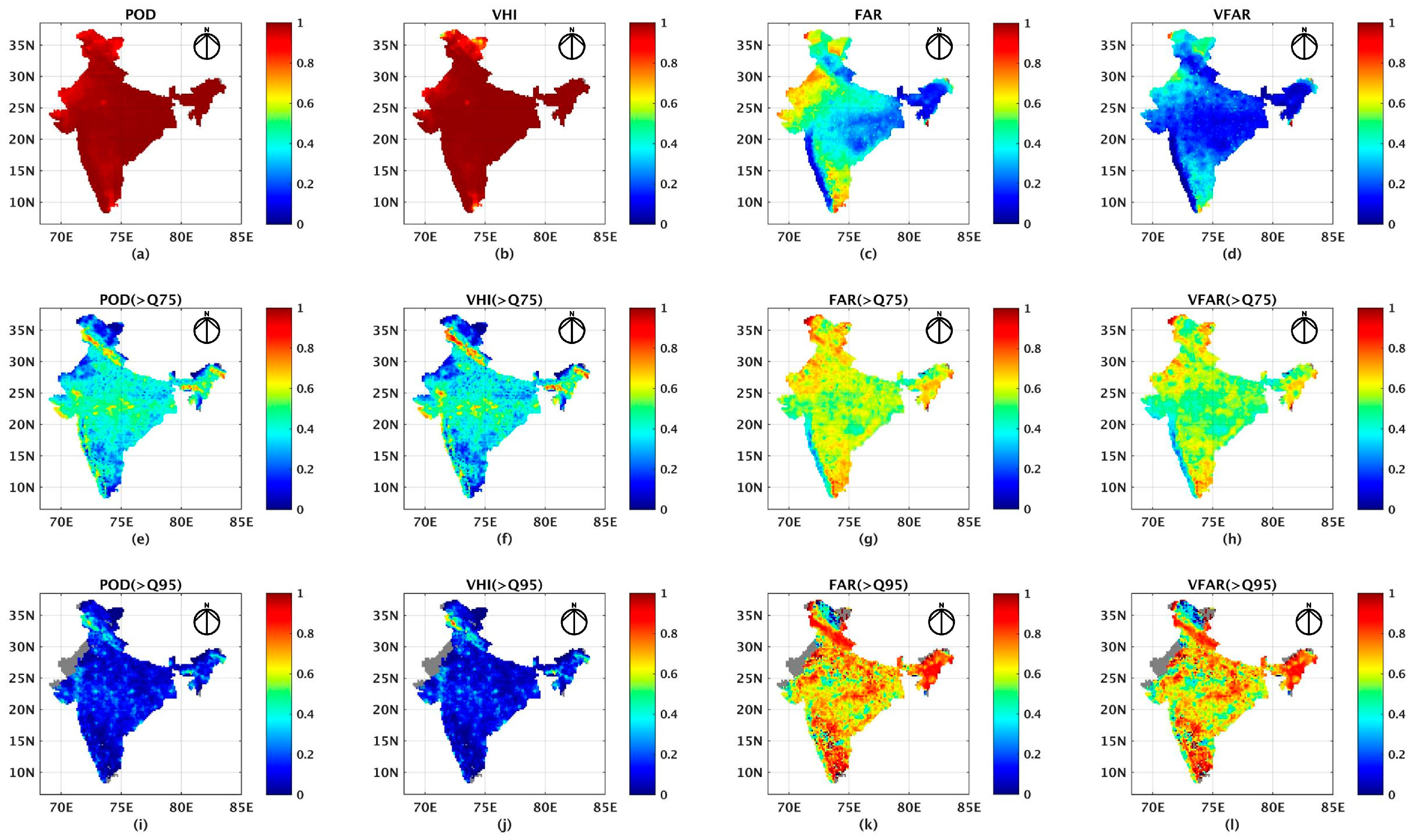
| 1. | Probability of Detection (POD) | |
| 2. | False Alarm Ratio (FAR) | |
| 3. | Critical Success index (CSI) | |
| 4. | Volumetric hit index (VHI) | |
| 5. | Volumetric False alarm ratio (VFAR) | |
| 6. | Volumetric miss index (VMI) | |
| 7. | Volumetric Critical Success index (VCSI) |
| Region | Climatological Mean Rainfall (mm/Day) | Daily Rainfall Mean for Monsoon Season (mm) | Root Mean Square Error (RMSE) (mm) | BIAS (mm) | Correlation Coefficient (CC) | ||
|---|---|---|---|---|---|---|---|
| IMD | MSWEP | IMD | MSWEP | ||||
| All India | 3.135 | 3.3096 | 7.1615 | 6.9751 | 0.1788 | −0.049 | 0.8605 |
| Southwest | 3.5006 | 3.2336 | 8.7101 | 7.3426 | 0.1953 | −0.043 | 0.8625 |
| Southeast | 2.4082 | 2.6388 | 3.0937 | 3.2343 | 0.1890 | −0.055 | 0.8589 |
| Central | 3.114 | 3.3577 | 8.1905 | 8.596 | 0.1947 | −0.060 | 0.8690 |
| Northwest | 1.3716 | 1.5297 | 3.595 | 3.9681 | 0.1901 | −0.056 | 0.8628 |
© 2017 by the authors. Licensee MDPI, Basel, Switzerland. This article is an open access article distributed under the terms and conditions of the Creative Commons Attribution (CC BY) license ( http://creativecommons.org/licenses/by/4.0/).
Share and Cite
Nair, A.S.; Indu, J. Performance Assessment of Multi-Source Weighted-Ensemble Precipitation (MSWEP) Product over India. Climate 2017, 5, 2. https://doi.org/10.3390/cli5010002
Nair AS, Indu J. Performance Assessment of Multi-Source Weighted-Ensemble Precipitation (MSWEP) Product over India. Climate. 2017; 5(1):2. https://doi.org/10.3390/cli5010002
Chicago/Turabian StyleNair, Akhilesh S., and J. Indu. 2017. "Performance Assessment of Multi-Source Weighted-Ensemble Precipitation (MSWEP) Product over India" Climate 5, no. 1: 2. https://doi.org/10.3390/cli5010002