Article

Trend and Homogeneity Analysis of Precipitation in Iran

College of Social Science, Payame Noor University, Tehran 19395-3697, Iran
Climate 2016, 4(3), 44; https://doi.org/10.3390/cli4030044
Submission received: 25 April 2016 / Revised: 21 August 2016 / Accepted: 1 September 2016 / Published: 8 September 2016

Abstract

:
The main objective of this study is to examine trend and homogeneity through the analysis of rainfall variability patterns in Iran. The study presents a review on the application of homogeneity and seasonal time series analysis methods for forecasting rainfall variations. Trend and homogeneity methods are applied in the time series analysis from collecting rainfall data to evaluating results in climate studies. For the homogeneity analysis of monthly, seasonal and annual rainfall, homogeneity tests were used in 140 stations in the 1975–2014 period. The homogeneity of the monthly and annual rainfall at each station was studied using the autocorrelation (ACF), and the von Neumann (VN) tests at a significance level of 0.05. In addition, the nature of the monthly and seasonal rainfall series in Iran was studied using the Kruskal-Wallis (KW) test, the Thumb test (TT), and the least squares regression (LSR) test at a significance level of 0.05. The present results indicate that the seasonal patterns of rainfall exhibit considerable diversity across Iran. Rainfall seasonality is generally less spatially coherent than temporal patterns in Iran. The seasonal variations of rainfall decreased significantly throughout eastern and central Iran, but they increased in the west and north of Iran during the studied interval. The present study comparisons among variations of patterns with the seasonal rainfall series reveal that the variability of rainfall can be predicted by the non-trended and trended patterns.

1. Introduction

Rainfall is an essential climatic element because it is the most important factor in the regionalization of climate and environmental conditions. In recent years, researchers reported temporal and spatial variability in rainfall across Asia including Iran. Furthermore, rainfall affects both the temporal and spatial patterns of climate variability. In the rainfall seasonality analysis in Iran, Talaee et al. (2014) noted that rainfall showed a decreasing trend in Iran in the previous years [1,2]. Some researchers [3,4,5,6,7] recognized indirect indications of trend and long-term variability of rainfall. Analysis of rainfall seasonality is important in investigating the influence of climate variability on the regional climate and environmental conditions [5]. Thus, the evaluation of trend or potential estimates on a regional scale is essential [8]. In this study, the trend and homogeneity of the rainfall series in Iran should be analyzed in order to discover any important variations in the rainfall pattern during 1975–2014. The seasonal rainfall patterns can be classified into two groups: trended seasonal patterns (TSP) and non-trended seasonal patterns (NSP). In trended seasonal data, the time series trended seasonal least squares methods (TSLSM) are used on the data from each station separately. In the non-trended seasonal patterns, the absolute seasonal least squares methods (ASLSM) are used on the data from each station individually. Likewise, the homogeneity tests could be divided into two groups: absolute tests and relative tests [1,9,10,11,12,13]. In this study, homogeneity tests were used: Pettit (1979), SNHT—Standard Normal Homogeneity Test (1986), Buishand (1982) and von Neumann (1941) tests [14,15]. The trend of rainfall is an essential aspect in the analysis of rainfall [4]. The variability of rainfall has an important effect on environmental processes. Another essential aspect of seasonal rainfall, namely the spatial pattern of seasonal rainfall, has been given little attention in Iran [2]. A climatic series is considered to have temporal patterns if there is a statistically significant relationship between the data and the season. Temporal changes in the rainfall data can be associated with the gradual change series for a short period and is often calculated by analyzing the monthly rainfall variability [5]. The trend in a time series can be described by a predictable long-term temporal model. However, temporal patterns are used in climatology rather than the cyclic and random ones. Various statistical methods have been used in the past to study trends in climatic data [16]. Trended and non-trended patterns are combined in this study to check the seasonal rainfall series. Various studies have applied homogeneity tests in recent years [9,12,13,15,17,18]. In climatic studies, trend and homogeneity were mainly checked contemporaneously in order to determine temporal patterns in rainfall [4,19]. Various statistical tests have been used to assess homogeneity in climatic series [9,12,13,17,18,20,21]. Actually, the applied parametric and nonparametric tests are based on several hypotheses, such as normality in the rainfall series [21,22,23,24]. Analysis and forecasting methods of time series show a seasonal pattern in different areas. There are various prediction methods in the analysis of time series [20,25,26]. In this study, the seasonal simple average (SSA), the seasonal least squares (SLS) and the seasonal Holt-winters (SHW) were used. Seasonal analysis is the forecast of a temporally distributed succession of seasonal data or the succession of a model for seasonal investigation wherein the period is an independent variable [27,28]. The seasonal simple average (SSA) is the most common approach to analyze the rainfall patterns. The seasonal least squares (SLS) method was used as a regression analysis tool in this study to fit trended and non-trended seasonal models and to analyze the rainfall series in Iran. Forecasts using least squares in additive and multiplicative models are important methods in modeling and forecasting rainfall data. The seasonal Holt-Winters as a seasonal smoothing and updating method is used in this study with an additive and multiplicative structure to analyze and forecast the rainfall series. The relationships between the spatial and temporal patterns of rainfall are investigated by extracting the seasonal layer from the time series using Trend Tools in the Spatial Analyst Tools of ArcGIS10.3 [29,30]. Precipitation variations in Iran can be quantified by the seasonal additive and multiplicative analysis of rainfall series. The main purpose of this paper is (1) to analyze precipitation homogeneity across Iran using the homogeneity tests; (2) to identify the spatial and temporal patterns of rainfall using seasonality methods and (3) to predict the possible rainfall variability patterns under climatic conditions. The results of this study could be used, for the management of climate and environmental conditions in Iran.

2. Study Area and Data

Iran is situated in the southwest of Asia, between 25°3′N to 39°47′N and 44°5′E to 63°18′E. The total area of Iran is approximately 1,348,195 km2. The climate of Iran is arid and semi-arid. The wet season usually starts from October and lasts for about six months up to the end of April. The study of the rainfall time series presented a seasonal pattern. In winter, the max of the rainfall (670 mm), spring (180 mm) and a min in summer (49 mm) and a second max in autumn (500 mm) show the decreasing pattern in summer whereas in winter and autumn, increasing pattern stations are found (Figure 1).
In this study, an analysis of the monthly, seasonal and annual rainfall in Iran was analyzed during the period 1975–2014, and recorded at 140 stations. Seasons were characterized as follows: winter (January, February, and March); spring (April, May and June); summer (July, August and September) and fall (October, November and December). We collected monthly and seasonal rainfall data from all of Iran 140 stations from the Islamic Republic of Iran Meteorological Office [31]: 38,968 rainfall points were extracted and processed to provide the rainfall layers of Iran using ArcGIS10.3 (Figure 2). For each station, a cell set of the input point’s raster dataset will be created in the output pattern class. The points will be positioned at the centers of stations where they are represented as an extracted layer. Any pattern class containing point (station) or multipoint class can be converted to a rainfall raster dataset. We used a statistic on the points in a neighborhood around each rainfall cell. The point statistics analysis performs a neighborhood procedure that calculates a rainfall raster layer where the value for each rainfall cell is a function of the values of any station point patterns that fall within a specified neighborhood around that location [32,33]. All the collected rainfall series were executed to testing normality and 140 detections were determined with trends and homogeneity. This paper analyzes the point statistical patterns of seasonal rainfalls in Iran observing for point patterns variability in the period’s (1975–2014) data series. Based on the point statistical analysis (Mean winter = 110.44 mm, standard deviation (SD) winter = 43.16 mm and mean spring = 50.2 mm, SD spring = 19.93 mm, mean summer = 2.88 mm, SD summer = 4.97 mm and mean autumn = 73.65 mm and SD autumn = 40.07 mm) rainfall variability showed the seasonal patterns.
The selected stations appears in Figure 2. Locally weighted scatterplot smoothing (LOWESS) was performed to remove general trends in the rainfall time series. Chambers et al. (1983) presented this method and provided some clear series. LOWESS is a smoothing method that uses an iterative locally weighted least squares method to fit a curve to a set of point rainfall series [34,35]. The monthly, seasonal and annual rainfall series for the 40-year period were applied to evaluate the temporal variation patterns in the rainfall series. In addition, to decrease the local oscillations, rainfall series were corresponded with the LOWESS curve (Figure 3) to detect temporal variation patterns in the rainfall series over time at annual and seasonal scales. In the present study, to evaluate rainfall distribution, we used the scatterplot corresponding with the LOWESS curve as shown in Figure 3. Moreover, all the rise and fall patterns taken from LOWESS curves (Figure 3A–E) as trend patterns appear in Figure 3.
In this analysis, various descriptive statistics of annual rainfall series were calculated for each station for the 1975–2014 period. In addition, the least squares method and the non-trended seasonal least squares and trended seasonal least squares methods were applied to the time series [2,13,28,36,37,38].

3. Methodology

In this study, the following methodological approach was implemented to investigate trend and homogeneity in the rainfall time series: (1) descriptive statistics of the annual rainfall series were used for each station over the period of 1975 to 2014; (2) series were checked for normality, homogeneity and trend by using parametric and nonparametric tests; (3) rainfall data were checked for selecting and describing the prediction models of the trend; and (4) forecasts of the temporal and spatial variations of the rainfall in Iran were provided.

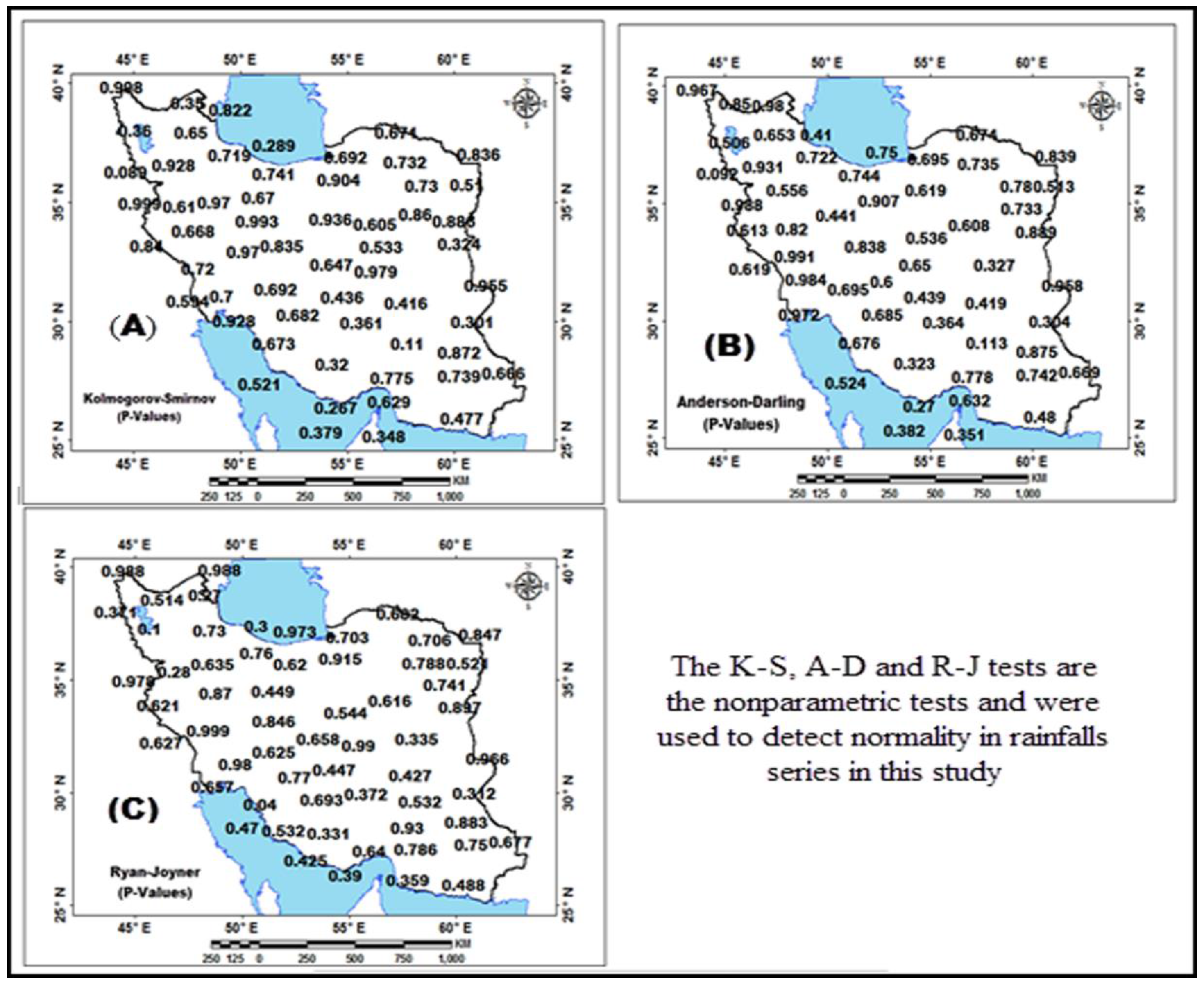
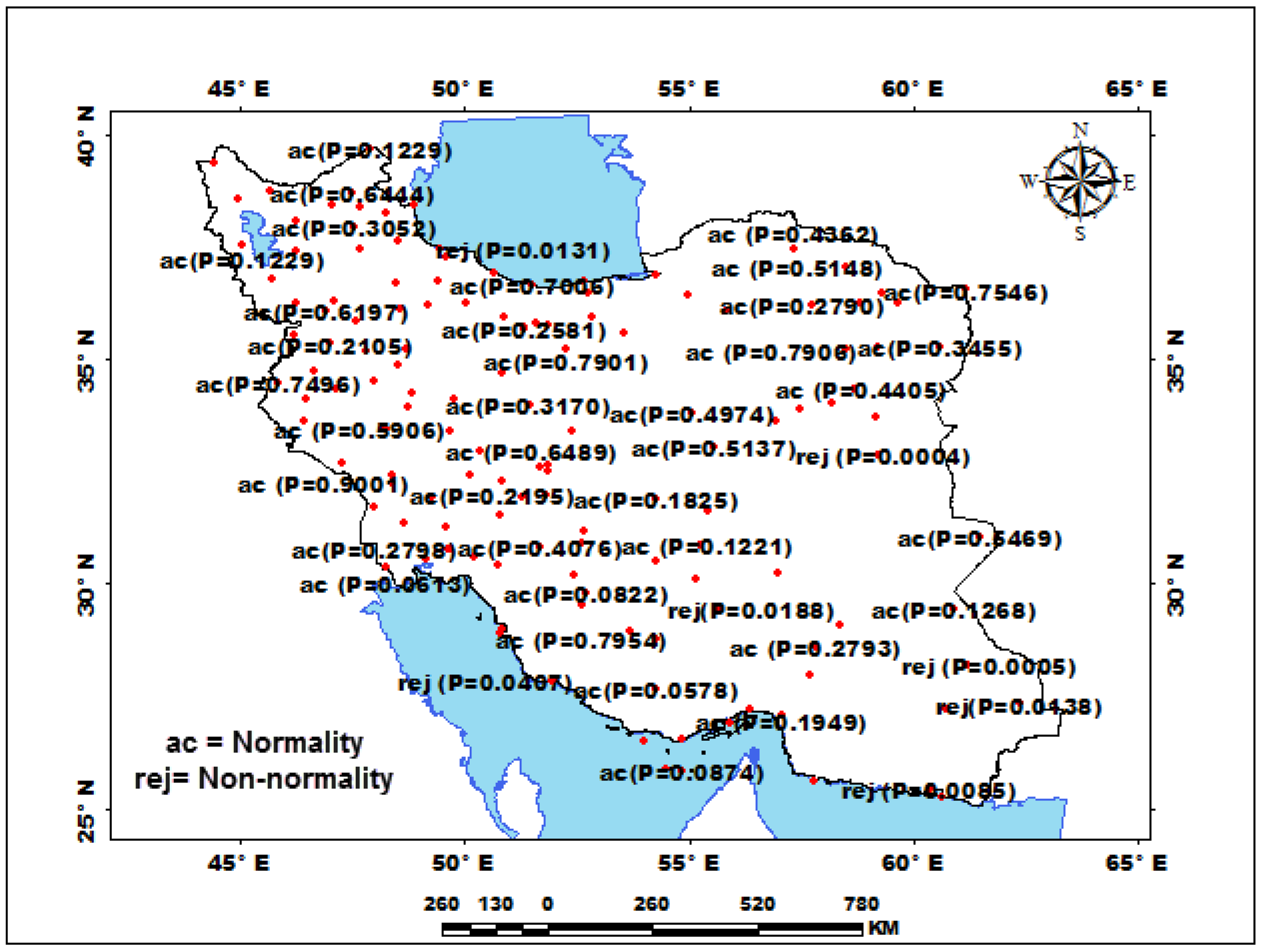
3.1. Checking the Normality and Homogeneity of Rainfalls Series

The statistical analyses of every climatic time series must always be carried out for studying important time series characters, i.e., normality, homogeneity, seasonality, presence of trends and changes, etc. Rainfall series of 140 stations across Iran were analyzed for the period of 1975–2014. We usually assume a sample is normally distributed in statistics. However, checking that this assumption is actually true is often ignored. There are both graphical and statistical methods for evaluating normality. In this study, the Anderson-Darling (A-D), Kolmogorov-Smirnov (K-S), Ryan-Joiner (R-J) and D’Agostino-Pearson (DA) tests were used to examine the normality of the rainfall series [21,37,39]. The Anderson-Darling test is used to test if a series comes from a population with a normal distribution. The value of A-D calculated is compared with the corresponding critical value of the theoretical distribution. The hypothesis that the distribution is normal is rejected if the value of A-D is greater than the critical value. [40]. The A-D test was applied to the data from each station. The K-S test is an empirical distribution function test in which the theoretical cumulative distribution function of the test distribution is compared with the empirical distribution function of the series. Large K-S values demonstrate the presence of non-normality in the time series. R-J test assesses normality by calculating the relationships between series and the normal scores of series. If the association coefficient is near 1, the data series is likely to be normal. The Ryan-Joiner statistic assesses the strength of this correlation; if it falls below the appropriate critical value, it will reject the null hypothesis of population normality. This test is similar to the Shapiro-Wilk normality test. The R-J test is similar to measuring a correlation between the quantity of the standard normal distribution and the ordered data points of a climatic series. For small values of the test-statistic, R-J demonstrates a departure from normality. The closer the obtained R-J is to 1, the closer the data distribution comes to a normal distribution; thus, if α > p , zero assumption is accepted based on the normality of the data. DA test first examines time series data to determine skewness (to calculate the normality of the data distribution) and kurtosis (to measure the shape of the data distribution). The DA test assumes approximately a chi-square distribution with two degrees of freedom under the hypothesis that the two series are independent and the population is normally distributed [21]. To measure the normality of the rainfall series, the Minitab and SPSS software were used. If normality exists in a rainfall series, a parametric test is selected. The results of the normality tests were interpreted by comparing the observed p-values, 0.05. If the p-value is more than 0.05—the null hypothesis—then normality is not rejected. It can be concluded from Table 1 that the observed p - values for the seasonal rainfalls are greater than 0.05 for the Kolmogorov-Smirnov test, the Anderson-Darling test, the Ryan-Joiner test and D’Agostino-Pearson test. Thus, based on the results of the normal probability test and the three normality tests, the rainfall series in this study can be considered normally distributed. Therefore, all the monthly rainfall series in this study are considered normally distributed. In climatic analysis, homogeneity is the most important characteristic of climatic time series. Homogeneity implies that the data in the series are similar and hence have no heterogeneous conditions. Homogeneity tests include a large number of tests for which the null hypothesis is that a time series is homogeneous between two given times. We used five homogeneity tests, the Pettitt-Whitney-Mann (PWM) [41], the Standard Normal Homogeneity Test or Alexandersson’s SNHT test [13], Buishand’s test [9], the autocorrelation test (ACF), and the von Neumann test (VN) to explore homogeneity in rainfall time series. The tests were applied at 5% significance level. The Pettitt's test is a nonparametric test that requires no hypothesis about the distribution of the data. The Pettitt’s test is an alteration of the tank-based Mann-Whitney test that allows detecting the time at which the change happens. The SNHT test (Standard Normal Homogeneity Test) was established by Alexandersson (1986) to identify a change in a series of rainfall data. Buishand’s test (1982) can be applied to a series with any kind of distribution. Nonetheless, its properties have been chiefly studied for normal distribution [1,12,13]. The von Neumann ratio (VN) is the most widely applied test for checking a time series for the existence of homogeneity [9,14]. However, it tends to be <2 for the non-homogeneous time series. We used the tests of normality for selection of parametric and nonparametric tests (normality assumption). The normality assumption is essential for the selection of tests, especially for parametric tests. Analyzing the results of the Pettitt-Whitney-Mann test shows the stations which are considered homogeneous for 40 years. In addition, rainfall amount at each of the 140 stations was tested for homogeneity by one absolute test method in, e.g., the von Neumann ratio of the precipitation series of each station by SYSTAT13 software. The von Neumann ratio of a discrete data was estimated as [23,26,28,42]:
M V = 2 n ( y t y t 1 ) 2 y 2 ( y ) 2 n
Test   rule :   Reject :   H 0 i f M V < M 1 α / 2 . The hypotheses of serial homogeneity were then tested by: Ho: ρk = 0 and Hα: ρk ≠ 0, using the test of significance of series autocorrelation. We conclude that there is a significant similarity variation across all the seasons. If lag-3 serial coefficients are not statistically significant, then the autocorrelation test can be applied to the original data. The autocorrelation coefficient r k of a discrete data was estimated as [22,23]:
r k = i = 1 n ( Y t k Y ¯ ) ( Y i Y ¯ ) ( Y i Y ¯ ) 2
where r k is the lag-k series autocorrelation coefficient. The hypotheses of series homogeneity were then tested by the lag-3 autocorrelation coefficient as: Ho: ρk = 0 and Hα: ρk ≠ 0, using the test of significance of serial correlation ( Reject :   H 0 i f | r k | > 2 / n ). The null hypothesis ( H 0 ) of serial homogeneity was rejected at the significance level α (0.05) [43,44]. The homogeneity of the annual and monthly precipitation series of Iran was studied using the autocorrelation and von Neumann tests. The results of each homogeneity test were analyzed for a significance level of 0.05. The analysis of the von Neumann test results shows that the stations with a test statistic lower than 1.49 (test rule: Reject: H 0 i f | 0.32 | < 1.49 ) are considered to be homogeneous for 40 years. (The critical values for tests can be obtained at degrees of freedom from the standard table available in textbooks on statistics.) The analysis of the autocorrelation test results indicates that the stations with a test statistic higher than 0.32 are considered to be homogeneous for 40 years.

3.2. The Decision to Use Seasonal Models

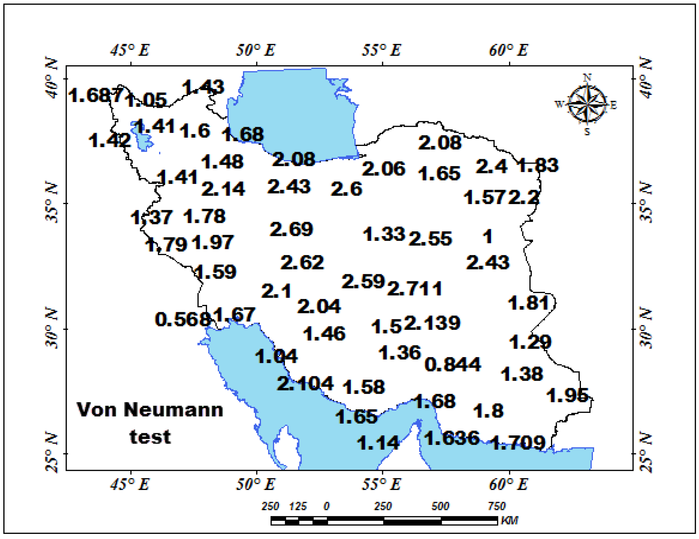
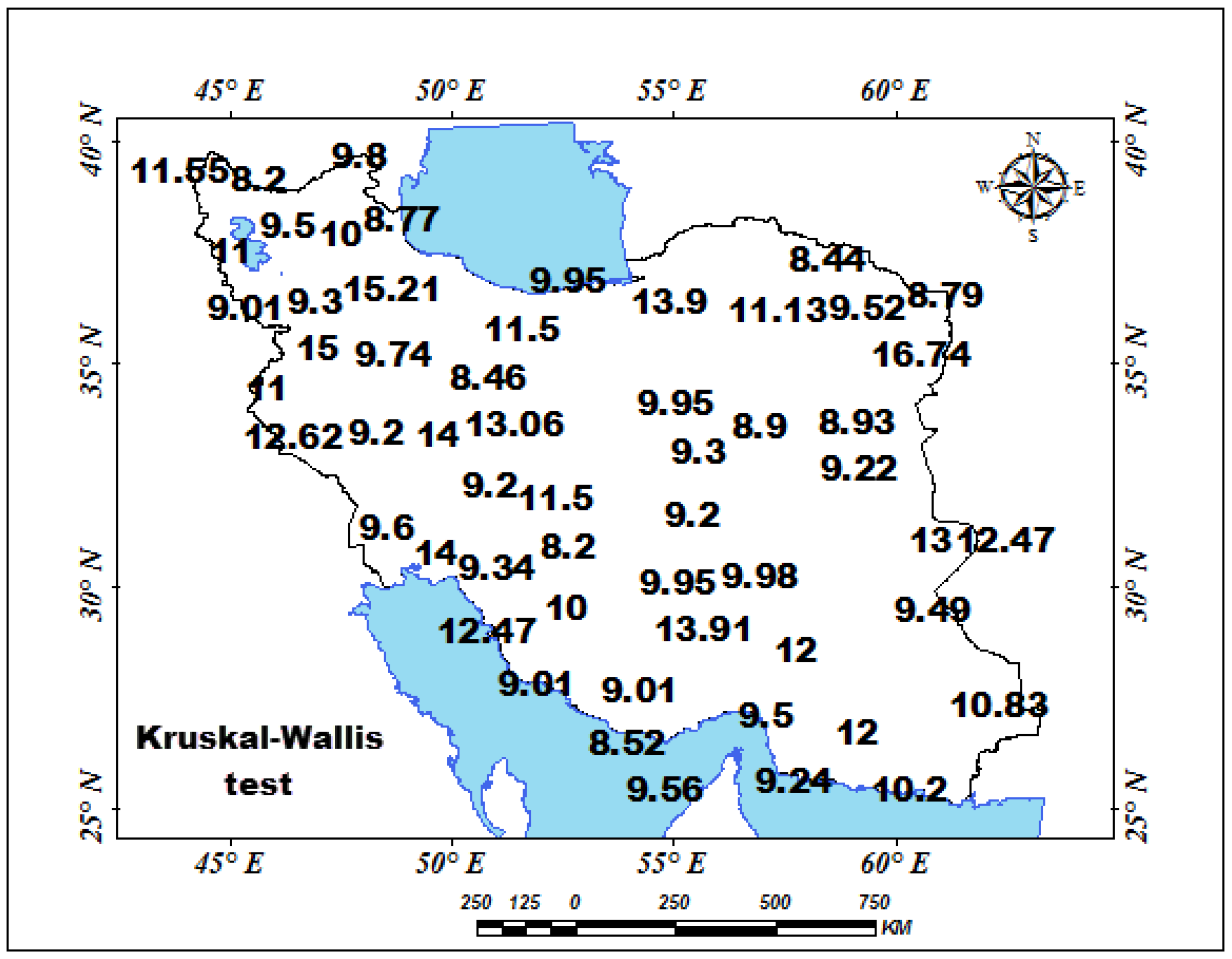
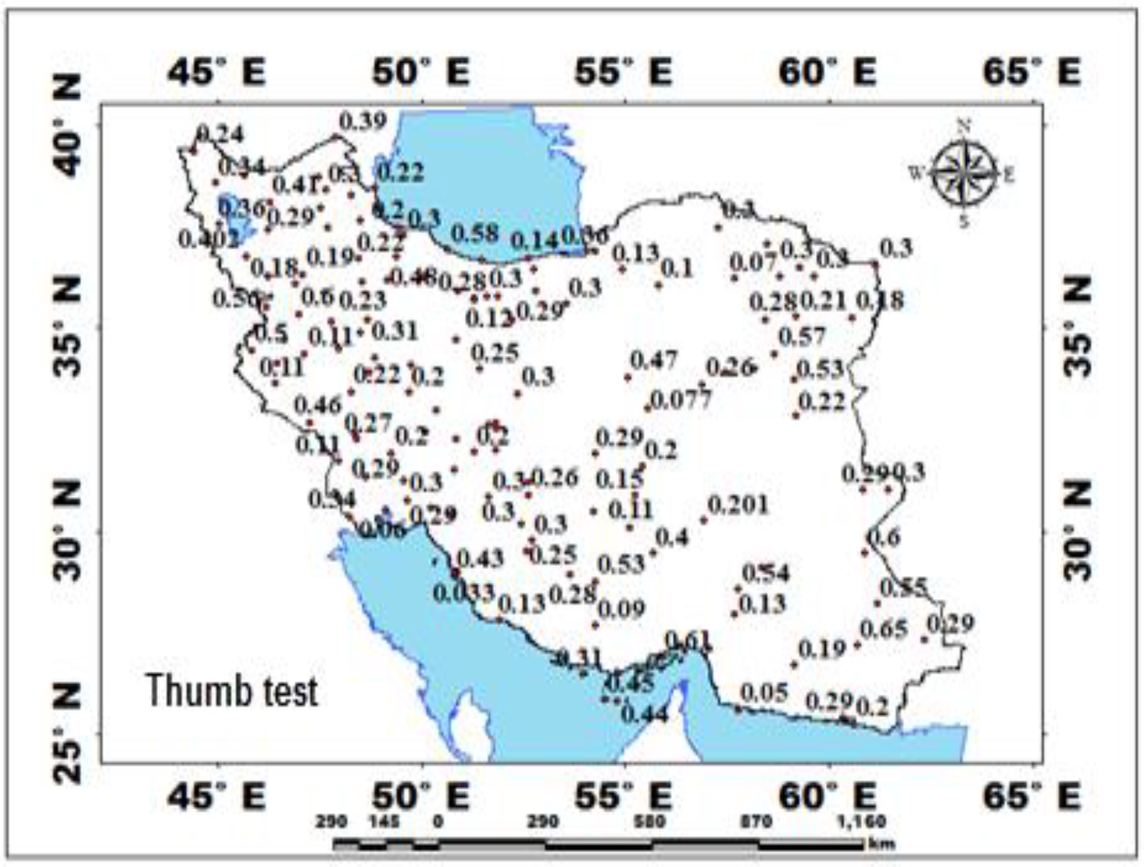
3.2.1. Application of Time Series Tests

In this study, time series are analyzed in order to determine the rainfall variability. Statistical tests are used to verify the presence/absence of trend and homogeneity in this study. In addition, ArcGIS is used to present spatial patterns of trend [45] and homogeneity in this study. Considering the nature of rainfall, two types of tests (parametric and nonparametric) are used for the time series analysis in order to facilitate decision-making. Statistical tests are applied in this study in order to ensure reliable measurements for time series forecasting. First, spatial and temporal variability in seasonal rainfalls of 140 stations are analyzed and forecasted using a 40-year (1975–2014) series. Then, seasonal rainfall time series of 140 stations for 40 years (1975–2014) are forecasted to detect seasonality by applying four statistical tests: Mann-Kendall test, for this test, we first calculate all Kendall's tau for each season, then calculate an average Kendall’s tau. The variance of the statistic can be calculated assuming that the series are independent or dependent, which requires the calculation of a covariance. The Mann-Kendall test (S) is given as follows [17,46,47]:
S = k = 1 n 1 j = k + 1 n sign ( x j x k )
where
sign ( x j x k ) = { + 1 if ( x j x k ) > 0 1 if ( x j x k ) < 0 0 if ( x j x k ) = 0
z = { s 1 v a r ( s ) . . if . . s > 0 0 .. if s = 0 s + 1 v a r ( s ) . . if . . s < 0
var ( s ) = n ( n 1 ) ( 2 n + 5 ) 18 . . if . n < 10
var ( s ) = n ( n 1 ) ( 2 n + 5 ) i 1 m t ( t 1 ) ( 2 t 5 ) 18
In this study, trend slope changes have been computed by percentage change. The change percentage is given as follows
P change ( % ) = β × t mean × 100
Thumb test is actually a process of self-comparison, expressing the seasonal correlation between an equally spaced series and the same series at a specified time lag or period. Thumb test statistic can be given by [23,26,48]:
r k = t = 0 n k ( x t . x t + k ) 1 / ( n k ) t = 0 n k x t . t = 0 n k x t + k [ t = 0 n k x t 2 1 / ( n k ) ( t = 0 n k x t ) ] 1 / 2 [ t = 0 n k x t + k 2 1 / ( n k ) ( t = 0 n k x t + k ) 2 ] 1 / 2
Decision rule of Thumb test is: Reject :   H 0 i f | r k | > Z α / n ) (the Kruskal-Wallis test was utilized on the seasonal rainfall), which is a serial version of the one-factor analysis rank statistic. The related test statistic can be given by [48,49]:
H = 12 n ( n + 1 ) [ R i 2 n i / n i ] 3 ( n + 1 )
Therefore, the hypothesis that the data are from all rainfall series with the null hypothesis is rejected, if Reject :   H 0 if | z τ | > Z α / 2 is the critical test-statistic value with d f = n 1 and a significance level of α) and least squares regression test. The least squares test statistic can be given by [23]:
Y t = β 0 + β 1 t + S 1 X 1 + S 2 X 2 + + S L X L + ε t   for   Additive
Y t = β 0 + β 1 t + ( S 1 ) X 1 + ( S 2 ) X 2 × × ( S L ) X L × ε t   for   Multiplicative
t = β ^ t ( S β 1 ^ )   for Trend
F = MSR ( S t ) MSE ( S t + T t )   for Seasonal
For the selected stations and rainfall data in the study area, the seasonal least squares test was used to distinguish the temporal trends of the seasonal rainfall series [21]. Spatial homogeneity of the annual rainfall time series is also examined by applying Levene’s analysis of variance test, von Neumann test and autocorrelation test [21,50]. These tests are performed using the SYSTAT13, SPSS and MINITAB software applications. Moreover, seasonal models (trended and non-trend) rainfall time series are controlled using the least squares regression test. Finally, the seasonality and homogeneity tests are used for all series with the 40-year data from 140 stations.

3.2.2. Application of Tests

The results confirm the existence of a seasonal pattern in Iran’s rainfall series. Checking the temporal variations pattern, Kruskal-Wallis (KW), Thumb (TT) and least squares regression (LSR) tests were applied to examine the trend of the rainfall series in this study [21,38]. For Kruskal-Wallis, if Ho is rejected, we conclude with ( 1 α ) × 100 % confidence that the series has seasonal variations. Thus, the Kruskal-Wallis test (nonparametric test) and the Thumb test (parametric test) determine the presence of a trend in all the rainfall series of Iran. The hypothesis test takes the form of Ho: the seasonal series is a non-trend series and Hα: the seasonal series has a trend. Rejection of Ho means there is sufficient evidence at the ( α 1 ) × 100 % confidence level that the seasonal series is trended. In addition, if the Thumb test result is positive, we conclude that the trend is increasing (upward); if the Thumb test result is negative, the trend is decreasing (downward). In addition, the least squares regression test (parametric test) determines the presence of series patterns (trended and non-trended) in all the rainfall series of Iran. Results of the least squares regression test are adjusted to the forecast series. Therefore, the results of the tests (i.e., Kruskal-Wallis (KW), Thumb (KT) and least squares regression (LSR) tests) are similar. In addition, to analyze the trend in the rainfall seasonal series, t-statistic is used as a parametric test. This is a parametric test, which assumes that the seasonal rainfall series is uncorrelated and normally distributed with mean and standard deviation. Critical amounts of this test-statistic can be taken from the Student’s t-distribution standard tables for n 2 degrees of freedom and 5% level of significance. If the calculated value of the test statistic is greater than its critical value, the null hypothesis is rejected and we conclude with ( 1 α ) × 100 % confidence that the rainfall seasonal series has a trend.

3.2.3. Forecast Models for Rainfalls Series

Seasonal forecasting of precipitation is a core competition for applied climatology. We present a method to develop forecasts for a time series that has a seasonal pattern. Forecasting involves basic definitions and assumptions. In this study, we have used least squares method or regression method [49] to predict rainfall patterns. However, we used the following steps: (1) Estimating the seasonal index. Seasonal index is an average that can be applied to evaluate an actual rainfall series relative to what it would be if there were no seasonal variations. An index amount is added to each period of the rainfall series within a year; (2) Seasonal adjustment of rainfall series; (3) Predicting the prevailing patterns into the future for the forecast of the trends using least squares; (4) Error assessment using the observed series and the predicted series. However, the method for seasonal forecasting has four stages: the application of measurement tests, the selection of analysis models, the selection of predictive model, the development of a control model for each station and season using seasonal models and the evaluation of forecast series. Forecasts using least squares in additive and multiplicative models are an important method for modeling and forecasting rainfall data. The least squares method can be used to fit trended or non-trended seasonal models to Iran series. The forecasts using least squares for Iran precipitation with additive and multiplicative models could be written in the following form for the additive model [23,28,38,51]:
Y ^ t = β ^ 0 + β ^ 1 t + S ^ 1 X 1 + S ^ 2 X 2 + + S ^ L X L
Model of least squares for multiplicative model:
Y ^ t = β ^ 0 + β ^ 1 t + ( S ^ 1 ) X 1 + ( S ^ 2 ) X 2 × × ( S ^ L ) X L
where S t is additive; multiplicative seasonal indexes, β 0 , β 1 t , are the constant coefficients for trend; and L is the length of the season. Problems with temporal patterns are common when the updating schemes are used for seasonal data. There are different methods of updated schemes. Here, we use the Holt-Winters model. Seasonal smoothing combined with a Holt-Winters linear-trend updating is usually called the Holt-Winters model or Holt-Winters smoothing (HWS). With an additive seasonal structure, the model is [40,42,52]:
Y t = ( β 0 + β 1 t ) + S t + ε t
Forecast for additive model:
Y ^ t + p ( t ) = T ^ t + p ( t ) + S ^ t + p ( t )
where S t is additive; multiplicative seasonal indexes, T t , are the trend component; ε t is the error; and β 0 , β 1 t are the constant coefficients for trend. The only change from the additive updating method for a multiplicative Holt-Winters model is in the way the seasonal adjustment and de-trending is performed, by division rather than subtraction. [26,53]. The Holt-Winters model is the most commonly used technique to predict the rainfall series. It is used when the data exhibit both trend and seasonal variations. In this study, the Holt-Winters technique is applied on the Iran rainfall series. The cross-validation used all the rainfall series to assess the non-trended and trended seasonal patterns. Cross-validation for each rainfall series location occurs one at a time and predicts the associated rainfall data value. Values of smoothing constants and (0.1) are optimized by minimizing mean absolute deviation (MAD), mean squared error (MSE), root mean squared error (RMSE) and mean absolute percent error (MAPE) indices using the solver tool of Microsoft Minitab. According to the accuracy indices analysis results, the MSE and RMSE (MSE(Multiplicative) = 5236.4, RMSE(Multiplicative) = 72.36 and MSE(Additive) = 4865.8, RMSE(Additive) = 69.76) indices for most of the stations in multiplicative updating of seasonality, is statistically more significant.

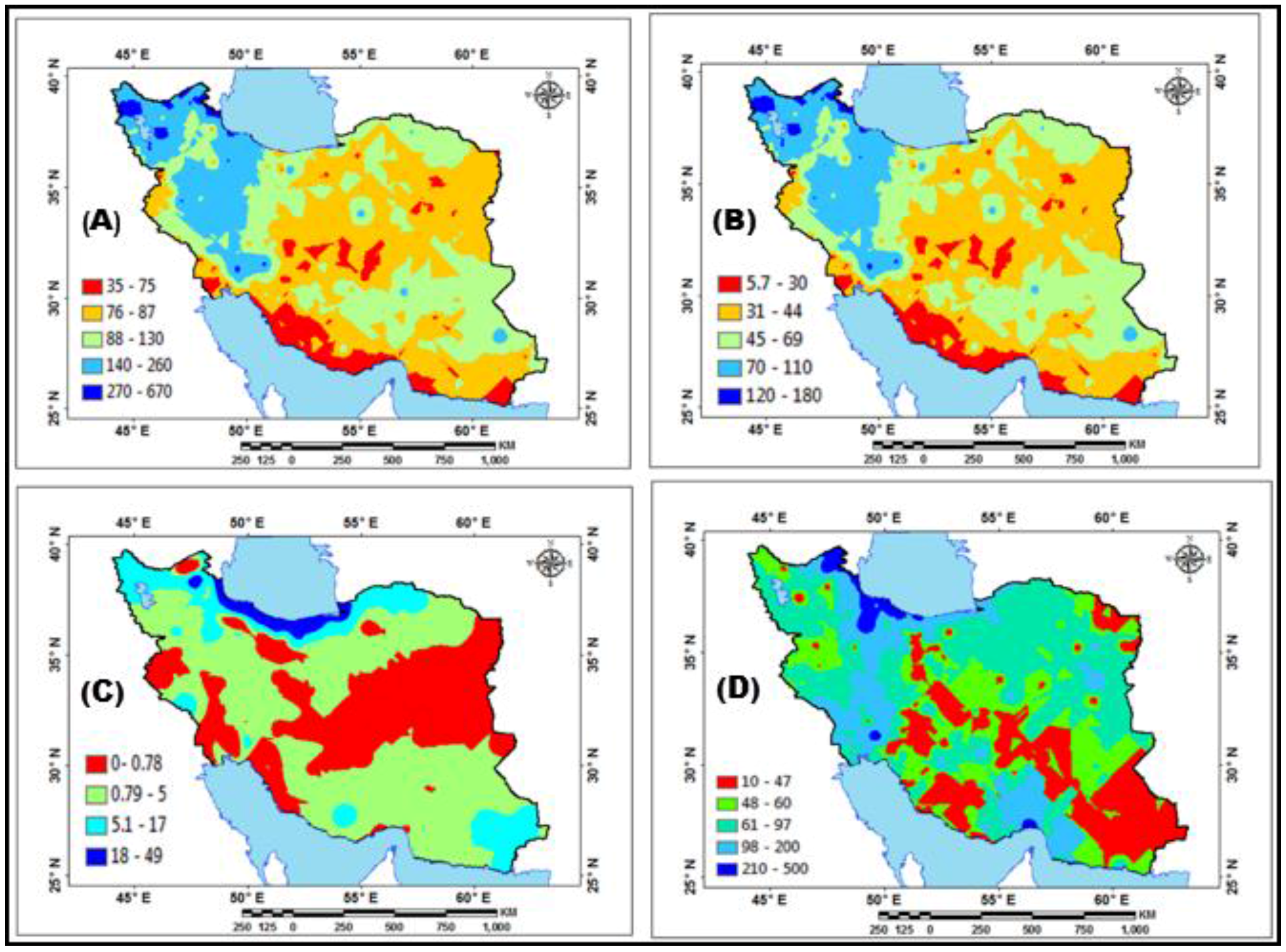
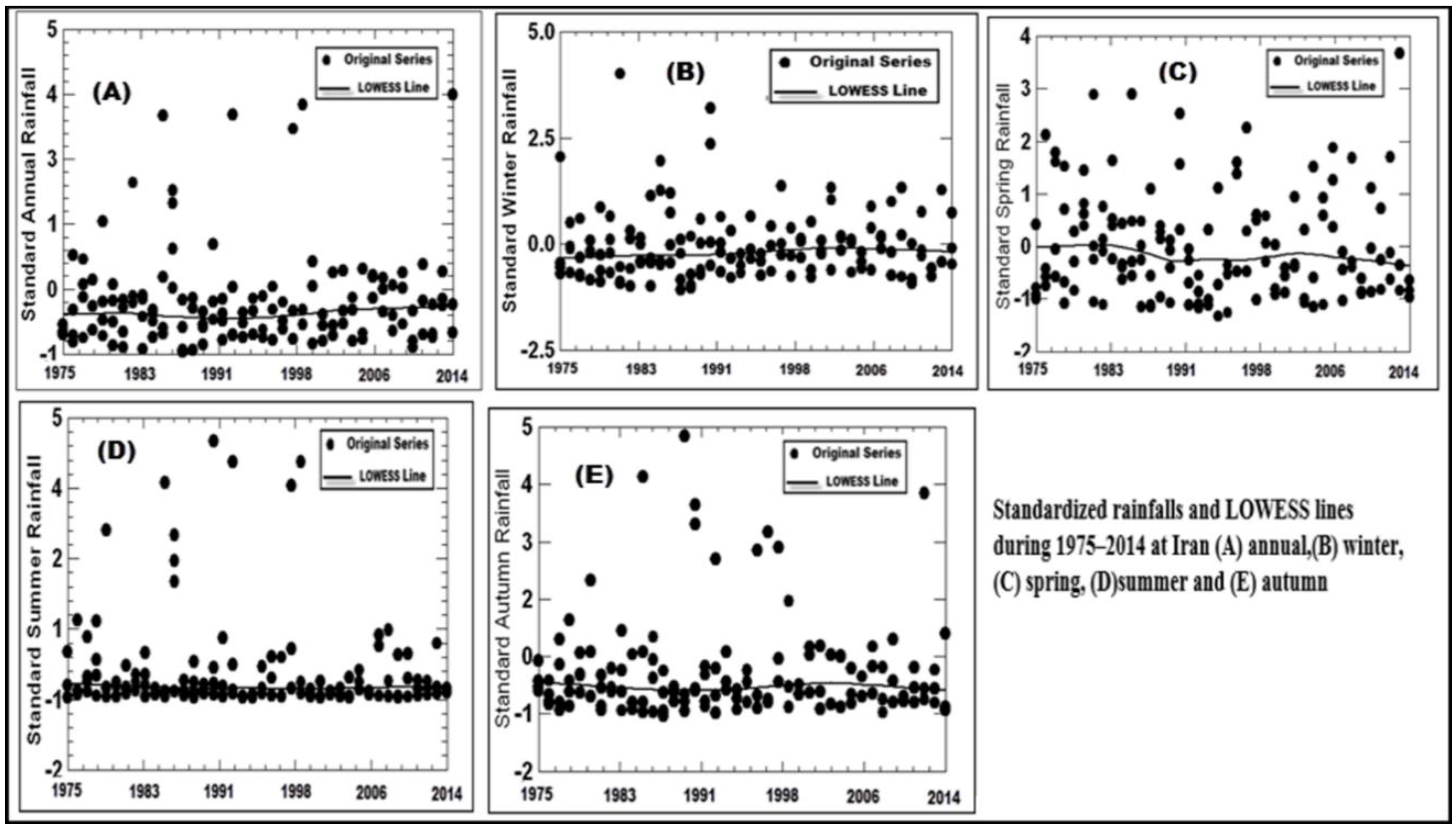
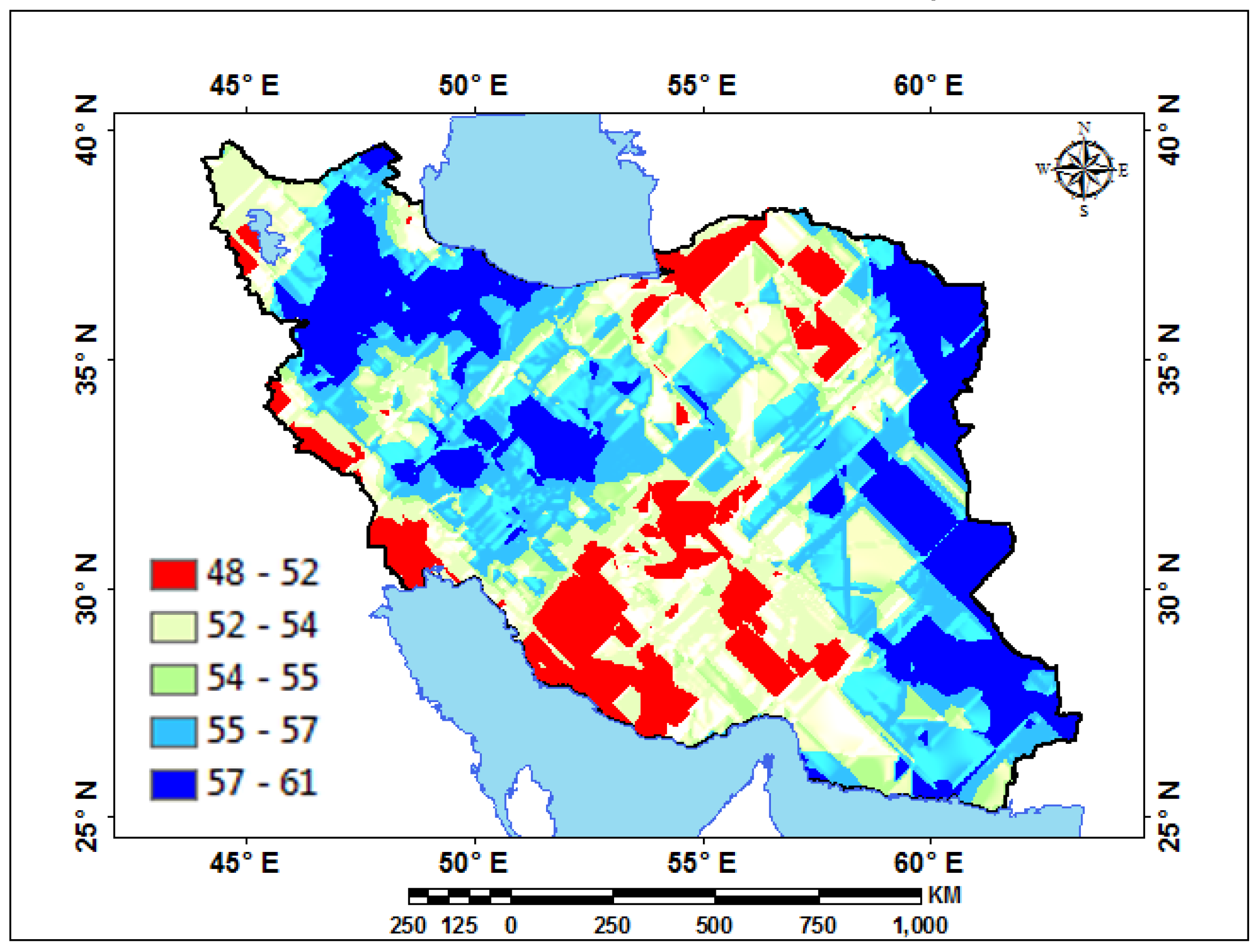
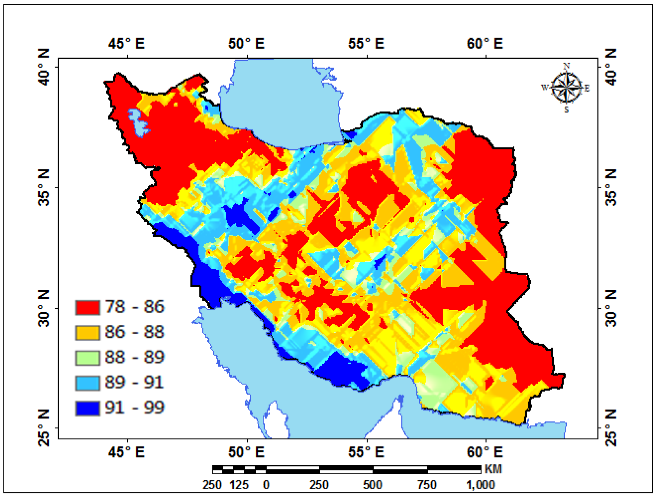
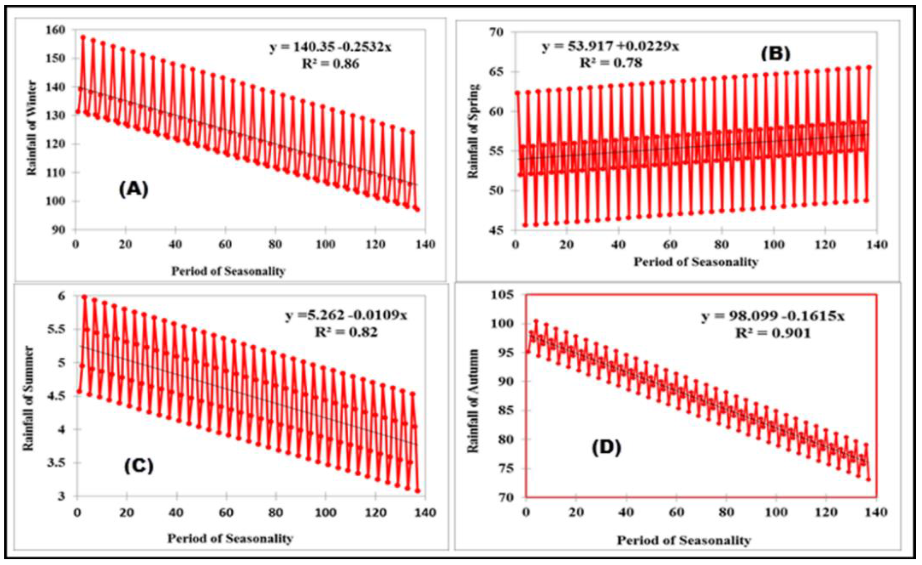
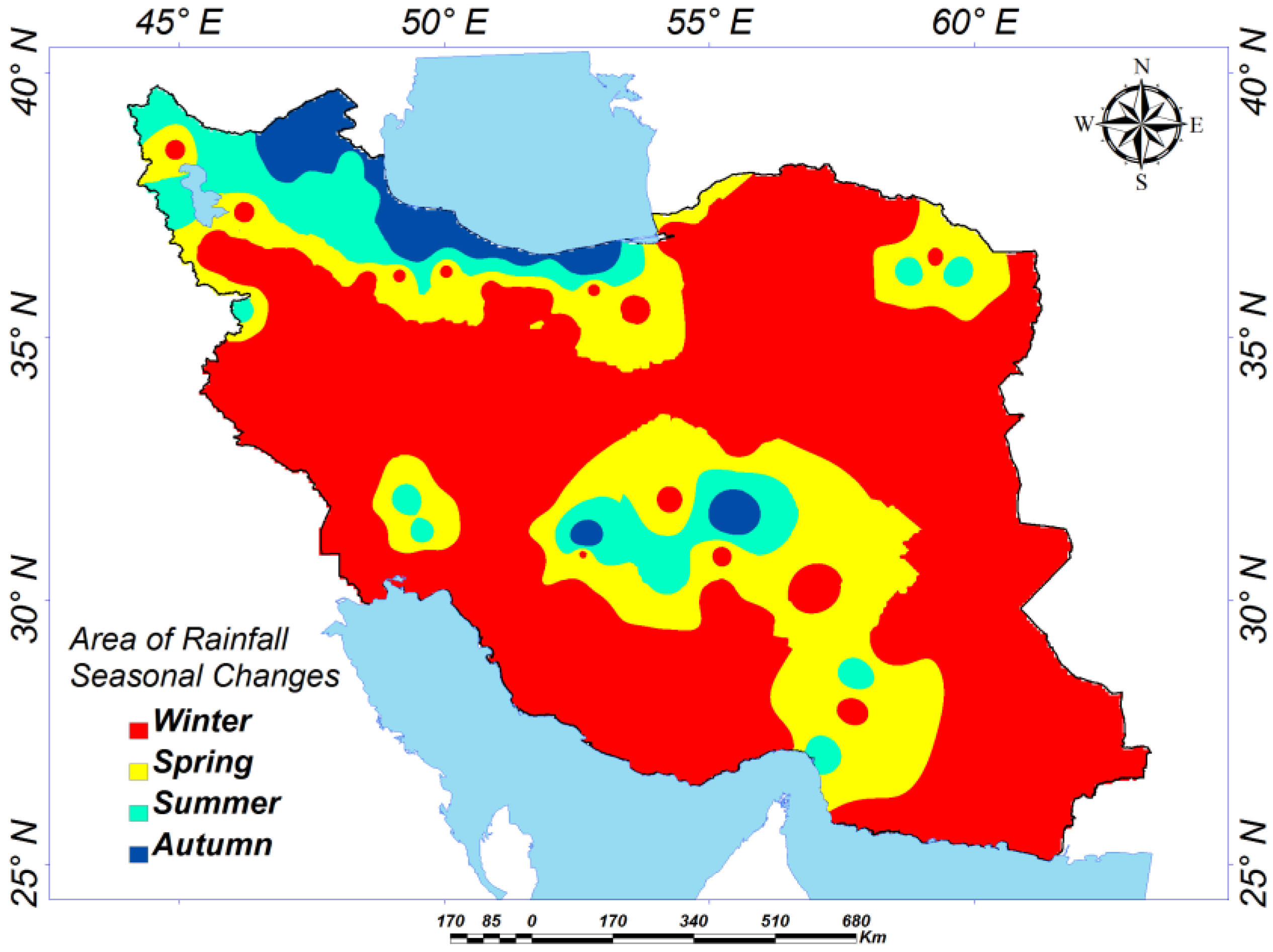
4. Results and Discussion

The LOWESS curve of annual rainfall presented a steady rise up to 1983 and reached the lowest value in 1991(Figure 3A). From 1991 onwards, it showed an upward trend up to 2014 and attained the highest value in 2014. The LOWESS curve of winter rainfall displayed a steady rise up to 2002 (Figure 3B) and reached the highest value in 2002. From 2002 onwards, it showed a downward trend up to 2014 and attained the lowest value in 2014.The LOWESS curve of spring rainfall displayed a steady fall up to 1990 (Figure 3C), reaching the lowest value in 1990. From 1990 onwards, it showed an upward trend up to 2004 and attained the lowest value in 2014. The LOWESS curve of summer rainfall displayed a steady fall up to 1990 (Figure 3D) and reached the lowest value in 1990. From 1990 onwards, it showed a steady and weak upward trend up to 2008 and attained the highest value in 2014. The LOWESS curve of autumn rainfall displayed a steady fall up to 1992 (Figure 3E), reaching the lowest value in 1992. From 1992 onwards, it showed a steady upward trend up to 2004 and attained the highest value in 2004 and reached the lowest value in 2014. However, curves show that Iran’s rainfall in the second half of the period tended to be smaller than that in the first half of the period. In this study, normality tests were used to analyze the nature of rainfall series. The various time series tests are performed to reveal the performance of these tests for analyzing and forecasting climatic time series through studying the monthly, seasonal and annual rainfall series of Iran. The normality testing and normal probability analysis of the rainfall series reveal no normality for some stations. The normal probability tests indicate normality in the monthly and annual rainfall series. However, the monthly and annual rainfall series are regarded as normally distributed. The results of these normality tests for all stations are also shown in Figure 4.
The normal distribution conditions indicate the conditions for selection of tests in the analysis of the monthly and annual rainfall series. The results of the D’Agostino-Pearson test are shown in Figure 5.
The homogeneity of the annual and monthly precipitation series of Iran is studied using the autocorrelation and von Neumann tests. The results of each homogeneity test are analyzed at a significance level of 0.05 and the results of the Pettitt-Whitney-Mann (PWM) test are shown in Table 1. The results of the Pettitt-Whitney-Mann test are indicated in the annual series of 112 stations and all the monthly precipitation stations are homogeneous. The results of the Alexandersson’s SNHT test of homogeneity are indicated in the annual series of 113 stations and all the monthly precipitation stations are homogeneous. The results of the SNHT test are shown in Table 2. The results of the Buishand’s test indicate homogeneity in the annual series of 114 stations and all the monthly precipitation stations are homogeneous. The results of Buishand’s test are shown in Table 3. The results of the von Neumann test indicate homogeneity in the annual series of 33 stations and all the monthly precipitation stations are homogeneous. The results of the von Neumann test are shown in Figure 6. The results of the autocorrelation test indicate homogeneity in the annual series of 28 stations and all the monthly precipitation stations are homogeneous.
The results of the autocorrelation test are shown in Figure 7. Furthermore, non-homogeneity created due to changes in the method of data collection over short periods are recorded for some stations.
Hence, it is thought that the annual rainfall series could be homogeneous. Based on the precision indicators, such as RMSE of the results of two homogeneity tests for the rainfall series, it can be suggested that the von Neumann test is better than the autocorrelation test. According to the analysis of von Neumann test results, the stations with a test statistic lower than 1.49 are considered homogeneous for the 40 years investigated. According to the analysis of the autocorrelation test results, the stations with a test statistic higher than 0.32 (the critical values for tests can be obtained at degrees of freedom from the standard table available in textbooks on statistics— ( Reject :   H 0 i f | 0.32 | < 1.49 ) are considered homogeneous for the studied interval [21]. The results of the von Neumann test in homogeneity are indicated in the annual series of 33 stations and all the monthly precipitation stations are homogeneous (Figure 6). The results of the autocorrelation test indicate homogeneity in the annual series of 28 stations and all the monthly precipitation stations are homogeneous (Figure 7). The seasonal variations of the monthly and seasonal precipitation series of Iran are studied using the Kruskal-Wallis (seasonal rainfall), Thumb (seasonal rainfall), and least squares regression tests (monthly rainfall). The results of each seasonality test are analyzed at a significance level of 0.05. The analysis of the Kruskal-Wallis test results shows that the stations with a test statistic higher than 7.81 (the critical values for tests can be obtained at degrees of freedom from the standard table available in textbooks on statistics— ( Reject :   H 0 if | H i n Figure . 8 | > X ( L 1 ) = 7.81 ) comprise a seasonal series for 40 years [21,54]. The results of the Kruskal-Wallis test are presented in Figure 8.
The analysis of the Thumb test results show that the stations with test values lower than 1.96 ( t = β ^ t ( S β 1 ^ )   for Trend , for seasonal series: { R e j e c t :   H 0 i f   | t | > t α / 2 t α / 2 = 1.96 ) exhibit seasonality for the 40 years of the study [21]. The results of the Thumb test are presented in Figure 9.
In this study, the nonparametric Mann-Kendall (MK) test was applied to distinguish trends. In addition, trend amounts (Z-values) have been computed by SYSTAT software. The number of stations in the MK test (Z-value), the results of the trend (positive and negative), and the 95% confidence level station are shown in Figure 10, independently of seasonal time scale rainfall series during 1975–2014.
Analysis of the seasonal rainfall series using MK test revealed 16 stations had a positive trend (16 of 140 stations or 11.43%) in winter and the rest had a negative trend (Figure 10); 27 stations had a positive trend (27 of 140 stations or 19.29%) in spring and the rest had a negative trend (Figure 10); 60 stations had a positive trend (60 of 140 stations or 42.86%) in summer and the rest had a negative trend (Figure 10); 26 stations had a positive trend (26 of 140 stations or 18.57%) in autumn and the rest had a negative trend (Figure 10); and 129 stations had a positive trend (129 of 140 stations or 92.1%) across all of Iran and the rest had a negative trend (Figure 10). In this study, t statistic   test ( t = β ^ t ( S β 1 ^ )   for Trend ) , for seasonal series: ( Reject :   H 0 if   | t | > t α / 2 t α / 2 = 1.96 ) and F test ( F = MSR ( S t ) MSE ( S t + T t )   for Seasonal ) —were used to generate the system of two similar parametric methods. The t test results indicate that the stations with test values higher than the p-value comprise a trended series and a seasonality series ( F test ) for 40 years. Otherwise, if the calculated value of the t statistic is less than its critical value at 5% level of significance with n–2 degrees of freedom, the null hypothesis of trend-free series cannot be rejected. Analysis of the seasonal precipitation series using t test found about 26.43% of the stations with a trended pattern (37 out of 140 stations) and 24 out of 137 or 65% stations have a downward trend (decreasing). The significant upward trend is found mostly in western and northern zones of Iran (Figure 10), whereas a significant downward trend is found in eastern and northeastern zones of Iran (Figure 11). The results of the seasonal tests are summarized in Figure 8, Figure 9 and Figure 10. It can be seen from these figures that the calculated test statistic values of all seasonal (for trended and no-trend patterns) tests are more than their critical values at the 5% level of significance (α = 0.05) in the rainfall series, which indicates the presence of a trend in some seasonal rainfall series of Iran. Negative test-statistic value of the seasonal data tests suggests a decreasing trend in the seasonal rainfall series of Iran. The results of the homogeneity tests indicating the presence/absence of homogeneity in the rainfall series of Iran are shown in Table 1, Table 2 and Table 3. According to von Neumann test, the monthly and annual rainfall at about 97% of the series are homogeneous, whereas the autocorrelation test indicates that only 93% of the series of monthly and annual rainfall have homogeneity in Iran. The temporal variability of the seasonal rainfall was studied to analyze the seasonal additive model of rainfall (Figure 11, Figure 12, Figure 13 and Figure 14). A statistically significant pattern of seasonality was observed in winter (Figure 11), spring (Figure 12), summer (Figure 13) and autumn (Figure 14) rainfall of the 40-year period. The seasonal changes slope of Iran precipitation (with additive model) varied between 0.921 and 1.165 mm in season per period. In general, in winter, there were wide declining precipitation trends over the past 40 years (Figure 11).
The seasonal changes of Iran precipitation (with additive model) varied between 108 and 139 mm in season per period during winter. The range of seasonal variations in spring precipitation varied between 0.340 and 0.625 mm in season per period (Figure 12).
The seasonal changes of Iran precipitation (with additive model) varied between 48 and 61 mm in season per period during spring. The range of seasonal eminency in summer precipitation varied between 0.134 and 0.167 mm in season per period (Figure 13).
Moreover, precipitation seasonal changes are observed with a 95% confidence level as 0.002 mm in season per period. The seasonal changes of Iran precipitation (with additive model) varied between 3.9 and 5 (dry season) mm in season per period during summer. The range of seasonal eminency in autumn precipitation varied between 0. 678 and 0.921 mm in season per period (Figure 14).
Thus, precipitation seasonal change with 95% confidence level is 0.016 mm/season per period. The seasonal changes of Iran’s precipitation (with additive model) varied between 3.9 mm during summer and 139 mm in season per period during winter. In addition, a statistically significant (R2 = 0.86) decrease was observed in winter (Figure 15a), summer (R2 = 0.82) (Figure 15c), and autumn (R2 = 0.901) (Figure 15d) and a statistically significant (R2 = 0.78) increase was observed in spring (Figure 15b) seasonal rainfall at the 5% level.
The results are in conformity with the trend pattern (decreasing) of the seasonal rainfall for the period 1975–2014 in winter, summer and autumn seasons. We observed that negative rainfall trends were 0.072 mm per decade in winter, 0.003 mm per decade in summer and 0.046 mm per decade in autumn. We also found that positive rainfall trends were 0.006 mm per decade in spring. A robust negative trend, up to 0.07 mm per decade, was detected in winter. Figure 16 shows the result of change percent of trend and forecasted seasonal rainfall using the seasonal prediction models.
The maximum decrease in trend changes percent in predicted seasonal rainfall was in summer (57.7%) followed by winter (53.5%), autumn (49.6%) and spring (32.4%) rainfall (9.87%) series. A robust negative trend, up to 0.031 mm per decade, was detected in the central, eastern and southern Iran and a robust positive trend, up to 0.006 mm per decade, was observed in northern and eastern Iran. The results in the area of forecasting the seasonal additive model are presented in Figure 17.
In general, seasonal variations are identified underneath the widely increasing precipitation patterns over the past 40 years.

5. Conclusions

This study demonstrates the application of statistical tests to determine trend and homogeneity in climatic series in Iran. In this study, both ArcGIS10.3 and statistical methods are used to determine spatial and temporal patterns in rainfall in Iran. In total, the spatial and temporal variations of monthly, seasonal and annual rainfall in this study are not statistically significant. It is also found that the monthly and annual rainfall time series are relatively more homogeneous compared to the seasonal time series. The results of the seasonal tests are almost similar. Homogeneity tests suggest that the monthly and annual series are homogeneous (more than 89% of series) in Iran. The results of the seasonal variations are shown for three distinct regions (north and northwestern, central, and coastal regions) and precipitation seasonal trends are also analyzed with the above methods. Smoothing techniques used in this approach are very effective, efficient and helpful to study load forecasting. In addition, the Holt-Winters model used in this approach exhibits better accuracy.

Acknowledgments

This research was supported by a grant from Payame Noor University. We also thank Payame Noor management and research committee of Payame Noor University.

Author Contributions

Seasonality and homogeneity analysis of precipitation in Iran was done by Majid Javari. All figures and tables were done by Majid Javari. Manuscript writing was made by Majid Javari.

Conflicts of Interest

The authors declare no conflict of interest.

References

  1. Talaee, P.H.; Kouchakzadeh, M.; Shifteh Some’e, B.S. Homogeneity analysis of precipitation series in Iran. Theor. Appl. Climatol. 2014, 118, 297–305. [Google Scholar] [CrossRef]
  2. Talaee, P.H. Iranian rainfall series analysis by means of nonparametric tests. Theor. Appl. Climatol. 2014, 116, 597–607. [Google Scholar] [CrossRef]
  3. Maussion, F.; Scherer, D.; Mölg, T.; Collier, E.; Curio, J.; Finkelnburg, R. Precipitation seasonality and variability over the Tibetan Plateau as resolved by the high Asia reanalysis. J. Clim. 2013, 27, 1910–1927. [Google Scholar] [CrossRef]
  4. Dhakal, N.; Jain, S.; Gray, A.; Dandy, M.; Stancioff, E. Nonstationarity in seasonality of extreme precipitation: A nonparametric circular statistical approach and its application. Water Resour. Res. 2015, 51, 4499–4515. [Google Scholar] [CrossRef]
  5. Pascale, S.; Lucarini, V.; Feng, X.; Porporato, A.; Hasson, S. Analysis of rainfall seasonality from observations and climate models. Clim. Dyn. 2015, 44, 3281–3301. [Google Scholar] [CrossRef]
  6. Keggenhoff, I.; Elizbarashvili, M.; Amiri-Farahani, A.; King, L. Trends in daily temperature and precipitation extremes over Georgia, 1971–2010. Weather Clim. Extremes 2014, 4, 75–85. [Google Scholar] [CrossRef]
  7. Powell, E.J.; Keim, B.D. Trends in daily temperature and precipitation extremes for the Southeastern United States: 1948–2012. J. Clim. 2014, 28, 1592–1612. [Google Scholar] [CrossRef]
  8. Hirsch, R.M.; Slack, J.R. A Nonparametric trend test for seasonal data With serial dependence. Water Resour. Res. 1984, 20, 727–732. [Google Scholar] [CrossRef]
  9. Buishand, T.A. Some methods for testing the homogeneity of rainfall records. J. Hydrol. 1982, 58, 11–27. [Google Scholar] [CrossRef]
  10. Sen, P.K. Estimates of the regression coefficient based on Kendall’s tau. J. Am. Stat. Assoc. 1968, 63, 1379–1389. [Google Scholar] [CrossRef]
  11. Santos, E.B.; Lucio, P.S.; Silva, C.M.S.E. Precipitation regionalization of the Brazilian Amazon. Atmos. Sci. Lett. 2015, 16, 185–192. [Google Scholar] [CrossRef]
  12. Wijngaard, J.; Klein Tank, A.; Können, G. Homogeneity of 20th century European daily temperature and precipitation series. Int. J. Climatol. 2003, 23, 679–692. [Google Scholar] [CrossRef]
  13. Alexandersson, H. A homogeneity test applied to precipitation data. J. Climatol. 1986, 6, 661–675. [Google Scholar] [CrossRef]
  14. Noureldin, D.; Shephard, N.; Sheppard, K. Multivariate rotated ARCH models. J. Econ. 2014, 179, 16–30. [Google Scholar] [CrossRef]
  15. Santos, M.; Fragoso, M. Precipitation variability in Northern Portugal: Data homogeneity assessment and trends in extreme precipitation indices. Atmos. Res. 2013, 131, 34–45. [Google Scholar] [CrossRef]
  16. Some’e, B.S.; Ezani, A.; Tabari, H. Spatiotemporal trends and change point of precipitation in Iran. Atmos. Res. 2012, 113, 1–12. [Google Scholar]
  17. Taxak, A.K.; Murumkar, A.R.; Arya, D.S. Long term spatial and temporal rainfall trends and homogeneity analysis in Wainganga basin, Central India. Weather Clim. Extremes 2014, 4, 50–61. [Google Scholar] [CrossRef]
  18. Singh, P.; Gupta, A.; Singh, M. Hydrological inferences from watershed analysis for water resource management using remote sensing and GIS techniques. Egypt. J. Remote Sens. Space Sci. 2014, 17, 111–121. [Google Scholar] [CrossRef]
  19. De Luis, M.; Čufar, K.; Saz, M.; Longares, L.; Ceglar, A.; Kajfež-Bogataj, L. Trends in seasonal precipitation and temperature in Slovenia during 1951–2007. Reg. Environ. Chang. 2014, 14, 1801–1810. [Google Scholar] [CrossRef]
  20. Montgomery, D.C.; Jennings, C.L.; Kulahci, M. Introduction to Time Series Analysis and Forecasting, 2nd ed.; John Wiley & Sons: Hoboken, NJ, USA, 2015. [Google Scholar]
  21. Kanji, G.K. 100 Statistical Tests, 3rd ed.; SAGE Publications Ltd.: Londan, UK, 2006. [Google Scholar]
  22. Machiwal, D.; Jha, M.K. Hydrologic Time Series Analysis: Theory and Practice; Springer: New York, NY, USA, 2012. [Google Scholar]
  23. Javari, M. Quantitative Methods in Climatology (Trend Models); Payam Resan Press: Tehran, Iran, 2010. [Google Scholar]
  24. Shapiro, S.S.; Wilk, M.B.; Chen, H.J. A comparative study of various tests for normality. J. Am. Stat. Assoc. 1968, 63, 1343–1372. [Google Scholar] [CrossRef]
  25. Kourentzes, N.; Petropoulos, F.; Trapero, J.R. Improving forecasting by estimating time series structural components across multiple frequencies. Int. J. Forecast. 2014, 30, 291–302. [Google Scholar] [CrossRef]
  26. Deepesh, M.; Jha, M.K. Hydrologic Time Series Analysis:Theory and Practice; Springer: New York, NY, USA, 2012. [Google Scholar]
  27. Zahradníček, P.; Rasol, D.; Cindrić, K.; Štěpánek, P. Homogenization of monthly precipitation time series in Croatia. Int. J. Climatol. 2014, 34, 3671–3682. [Google Scholar] [CrossRef]
  28. Brockwell, P.J.; Davis, R.A. Time Series: Theory and Methods; Springer Science & Business Media: Berlin, Germany, 2013. [Google Scholar]
  29. Moran, P.A.P. Notes on continuous stochastic phenomena. Biometrika 1950, 37, 17–23. [Google Scholar] [CrossRef]
  30. Johnston, K.; Ver Hoef, J.M.; Krivoruchko, K.; Lucas, N. Using ArcGIS Geostatistical Analyst; Esri Redlands, 2001. [Google Scholar]
  31. IRIMO. Islamic Republic of Iran Meteorological Office. Available online: http://www.irimo.ir (accessed on 6 September 2016).
  32. Xu, G.; Jiao, L.; Zhao, S.; Cheng, J. Spatial and temporal variability of PM2.5 concentration in China. Wuhan Univ. J. Nat. Sci. 2016, 21, 358–368. [Google Scholar] [CrossRef]
  33. Javari, M. Spatial neighborhood analysis of the monthly rainfall in Iran. Geoinfor. Geostat. Overv. 2015, 18, 1975–2014. [Google Scholar]
  34. Chambers, J.M.; Cleveland, W.S.; Kleiner, B.; Tukey, P.A. Graphical Methods for Data Analysis, 1st ed.; Wadsworth International Group: Belmont, CA, USA, 1983. [Google Scholar]
  35. Neteler, M.; Bowman, M.H.; Landa, M.; Metz, M. GRASS GIS: A multi-purpose open source GIS. Environ Model Softw. 2012, 31, 124–130. [Google Scholar] [CrossRef]
  36. Shumway, R.H.; Stoffer, D.S. Time Series Analysis and its Applications, 3rd ed.; Springer Science & Business Media: Berlin, Germany, 2013. [Google Scholar]
  37. Yue, S.; Pilon, P.; Cavadias, G. Power of the Mann-Kendall and Spearman’s rho tests for detecting monotonic trends in hydrological series. J. Hydrol. 2002, 259, 254–271. [Google Scholar] [CrossRef]
  38. Farnum, R.N.; Staton, L.W. Quantitative Forecasting Methods; Pws Pub Co.: Boston, MA, USA, 1989. [Google Scholar]
  39. Mann, H.B. Nonparametric tests against trend. Econ. J. Econ. Soc. 1945, 13, 245–259. [Google Scholar] [CrossRef]
  40. Goswami, B.; Venugopal, V.; Sengupta, D.; Madhusoodanan, M.; Xavier, P.K. Increasing trend of extreme rain events over India in a warming environment. Science 2006, 314, 1442–1445. [Google Scholar] [CrossRef] [PubMed]
  41. Pettitt, A.N. A Non-Parametric Approach to the Change-Point Problem. J. R. Stat. Soc. Ser. C (Appl. Stat.) 1979, 28, 126–135. [Google Scholar] [CrossRef]
  42. McCuen, R.H. Modeling Hydrologic Change: Statistical Methods; CRC Press Company: Boca Raton, London, UK, 2003. [Google Scholar]
  43. Pohlmann, H. Geostatistical modelling of environmental data. CATENA 1993, 20, 191–198. [Google Scholar] [CrossRef]
  44. Lillesand, T.; Kiefer, R.W.; Chipman, J. Remote Sensing and Image Interpretation; John Wiley & Sons: Hoboken, NJ, USA, 2014. [Google Scholar]
  45. Javari, M. Geostatistical and spatial statistical modelling of precipitation variations in Iran. J. Civ. Environ. Eng. 2016, 6, 1–30. [Google Scholar] [CrossRef]
  46. Kumar, V.; Jain, S.K.; Singh, Y. Analysis of long-term rainfall trends in India. Hydrol. Sci. J. 2010, 55, 484–496. [Google Scholar] [CrossRef]
  47. Stoffer, D.S.; Shumway, R.H. Time Series Analysis and Its Application: With R Examples; Springer Science & Business Media: Berlin, Germany, 2000. [Google Scholar]
  48. North, G.R. Statistical methods|data analysis: Time series analysis. In Encyclopedia of Atmospheric Sciences, 2nd ed.; Zhang, G.R.N.P., Ed.; Academic Press: Deditor Oxford, UK, 2015; pp. 205–210. [Google Scholar]
  49. Woody, J. Time series regression with persistent level shifts. Stat. Probab. Lett. 2015, 102, 22–29. [Google Scholar] [CrossRef]
  50. Zeng, X.; Wang, D.; Wu, J. Comparisons of Methods of Goodness of Fit Tests in Hydrologic Analysis; CRC Press: Boca Raton, FL, USA, 2015. [Google Scholar]
  51. Ifeka, A.; Akinbobola, A. Trend analysis of precipitation in some selected stations in Anambra State. Atmos. Clim. Sci. 2015, 5, 1–12. [Google Scholar] [CrossRef]
  52. Khashei, M.; Rafiei, F.M.; Mirahmadi, A. Seasonal interval time series models in comparative study of industrial forecasting. Int. J. Curr. Trends Eng. Technol. 2015, I, 51–58. [Google Scholar]
  53. Becketti, S. Introduction to Time Series Using Stata; Stata Press Books: College Station, TX, USA, 2013. [Google Scholar]
  54. Grimaldi, S.; Kao, S.C.; Castellarin, A.; Papalexiou, S.M.; Viglione, A.; Laio, F.; Aksoy, H.; Gedikli, A. 2.18-statistical hydrology. In Treatise on Water Science; Wilderer, P., Ed.; Elsevier: Oxford, UK, 2011; pp. 479–517. [Google Scholar]
Figure 1. Rainfall seasonal distribution in Iran: (A): Winter; (B): Spring; (C): Summer and (D): Autumn.
Climate 04 00044 g001
Figure 2. Selected stations.
Climate 04 00044 g002
Figure 3. Standardized rainfall series and LOWESS lines during 1975–2014 in Iran (A) annual; (B) winter; (C) spring; (D) summer and (E) autumn.
Climate 04 00044 g003
Figure 4. Results of K-S (A); A-D (B) and R-J (C) tests for rainfall in Iran.
Climate 04 00044 g004
Figure 5. Results of D’Agostino-Pearson test for rainfall in Iran.
Climate 04 00044 g005
Figure 6. Values of the von Neumann test.
Climate 04 00044 g006
Figure 7. Values of the autocorrelation test.
Climate 04 00044 g007
Figure 8. Values of Kruskal-Wallis test.
Climate 04 00044 g008
Figure 9. Values of the Thumb test.
Climate 04 00044 g009
Figure 10. Seasonal trend analysis of rainfall in Iran.
Climate 04 00044 g010
Figure 11. Forecast of winter rainfall variations (seasonal additive model).
Climate 04 00044 g011
Figure 12. Forecast of spring rainfall variations (seasonal additive model).
Climate 04 00044 g012
Figure 13. Forecast of summer rainfall variations (seasonal additive model).
Climate 04 00044 g013
Figure 14. Forecast of autumn rainfall variations (seasonal additive model).
Climate 04 00044 g014
Figure 15. Temporal distribution of rainfall seasonal trends in Iran. (a) Winter; (b) spring; (c) summer; (d) autumn.
Climate 04 00044 g015
Figure 16. Trend changes percent of forecasted seasonal rainfall.
Climate 04 00044 g016
Figure 17. Area of rainfall seasonal variations (additive).
Climate 04 00044 g017
Table 1. Results of PWM test for rainfall in Iran.
StationPettitt Test-p-ValueStationPettitt Test-p-ValueStationPettitt Test-p-ValueStationPettitt Test-p-ValueStationPettitt Test-p-ValueStationPettitt Test-p-Value
ABADAN0.062BOROOJEN0.821GHORVEH0.215KHALKHAL0.698NEYSHABOOR0.023SHAHROUD0.061
ABADEH0.082BOSHROOY0.101GOLMAKAN CHENARAN0.745KHASH0.434NOUSHAHR0.760SHARGH ESFAHAN0.523
ABALI0.939BOSTAN0.321GONABAD0.089KHODABANDEH0.472OMIDIYEH (PAYGAH)0.442SHIRAZ0.277
AHAR0.115BROUJERD0.156GORGAN0.004KHOOR BIABANAK0.002OMIDIYEH (AGHAJARI0.598SHOMALE TEHRAN0.872
AHWAZ0.327BUSHEHR (COASTAL)0.210HAMEDAN FOROUDGAH0.529KHORRAMABAD0.203OROOMIEH0.030SIRJAN0.149
ALIGOODARZ0.930BUSHEHR0.501HAMEDAN NOZHEH0.311KHORRAMDAREH0.559PARSABADE-MOGHAN0.679TABASS0.828
ANAR0.179CHAHBAHAR0.493HASANABADE DARAB0.121KHOY0.004RAMHORMOZ0.120TABRIZ0.001
ARAK0.056DARAN0.736ILAM0.055KOOHRANG0.324RAMSAR0.566TAKAB0.025
ARDEBIL0.001DEHLORAN0.081IRANSHAHR0.277LAR0.279RASHT0.474TEHRAN MEHRABAD0.214
ARDESTAN0.318DEZFUL0.696JASK0.035LORDEGAN0.702RAVANSAR0.159TORBATE HEYDARIEH0.370
ASTARA0.082DOGONBADAN0.460JAZIREH ABOMOOSA0.483MAHABAD0.256ROBAT POSHTBADAM0.913TORBATE JAM0.109
BABOLSAR0.053DOUSHAN TAPPEH0.903JAZIREH GHESHM0.091MAKOO0.182SABZEVAR0.035YASOUJ0.534
BAFGH0.366EGHLIDE FARS0.469JAZIREH KISH0.027MALAYER0.886SAD DOROUDZAN0.379YAZD0.412
BAM0.057ESFAHAN0.327JAZIREH SIRI0.795MANJIL0.487SAFIABAD0.345ZABOL0.093
B. ABASS0.257ESLAMABAD GHARB0.022JOLFA0.401MARAGHEH0.003SAGHEZ0.025ZAHEDAN0.010
B. ANZALI0.061FASSA0.518KABOOTARABAD0.716MARIVAN0.046SANANDAJ0.004ZANJAN0.290
B. DAIER0.611FERDOUS0.021KAHNOUJ0.113MARVAST0.279SAR POL ZOHAB0.002ZARGHAN0.008
B.LENGEH0.118FIROUZKOOH0.190KANGAVAR0.497MASHHAD0.489SARAB0.363ZARINEHO0.250
B.MAHSHAHR0.139GARMSAR0.514KARAJ0.583MASJED SOLEYMAN0.045SARAKHS0.348ZAHAK0.061
BEHBAHAN0.616GHAEN0.013KASHAN0.725MESHKINSHAHR0.231SARAVAN0.123ZARINEH OBATO0.523
BIARJAMAND0.385GHARAKHIL GHAEMSHR0.961KASHMAR0.281MIANDEH JIROFT0.001SEMNAN0.627Pettitt test-p-value
BIJAR0.001GHAZVIN0.545KENARAK0.466MIANEH0.327SHAHR BABAK0.060
BIRJAND0.298GHOM0.342KERMAN0.020MINAB0.602SHAHREKORD0.667
BOJNURD0.604GHOOCHAN0.658KERMANSHAH0.217MOSHIRAN0.240SHAHREZA0.289
Table 2. Results of SHHT test for rainfall in Iran.
StationSHHT Test-p-ValueStationSHHT Test-p-ValueStationSHHT Test-p-ValueStationSHHT Test-p-ValueStationSHHT Test-p-ValueStationSHHT Test-p-Value
ABADAN0.328BOROOJEN0.251GHORVEH0.416KHALKHAL0.920NEYSHABOOR0.008SHAHROUD0.226
ABADEH0.742BOSHROOY0.310GOLMAKAN CHENARAN0.966KHASH0.581NOUSHAHR0.528SHARGH ESFAHAN0.672
ABALI0.739BOSTAN0.270GONABAD0.197KHODABANDEH0.924OMIDIYEH (PAYGAH)0.557SHIRAZ0.006
AHAR0.302BROUJERD0.100GORGAN0.109KHOOR BIABANAK0.001OMIDIYEH (AGHAJARI0.338SHOMALE TEHRAN0.824
AHWAZ0.366BUSHEHR (COASTAL)0.337HAMEDAN FOROUDGAH0.514KHORRAMABAD0.268OROOMIEH0.033SIRJAN0.274
ALIGOODARZ0.768BUSHEHR0.100HAMEDAN NOZHEH0.410KHORRAMDAREH0.540PARSABADE-MOGHAN0.136TABASS0.618
ANAR0.056CHAHBAHAR0.703HASANABADE DARAB0.080KHOY0.027RAMHORMOZ0.046TABRIZ0.008
ARAK0.175DARAN0.825ILAM0.074KOOHRANG0.182RAMSAR0.761TAKAB0.020
ARDEBIL0.009DEHLORAN0.249IRANSHAHR0.480LAR0.319RASHT0.215TEHRAN MEHRABAD0.332
ARDESTAN0.309DEZFUL0.302JASK0.163LORDEGAN0.325RAVANSAR0.456TORBATE HEYDARIEH0.266
ASTARA0.203DOGONBADAN0.342JAZIREH ABOMOOSA0.550MAHABAD0.444ROBAT POSHTBADAM0.563TORBATE JAM0.370
BABOLSAR0.201DOUSHAN TAPPEH0.724JAZIREH GHESHM0.002MAKOO0.132SABZEVAR0.080YASOUJ0.105
BAFGH0.278EGHLIDE FARS0.496JAZIREH KISH0.071MALAYER0.892SAD DOROUDZAN0.173YAZD0.492
BAM0.056ESFAHAN0.195JAZIREH SIRI0.600MANJIL0.056SAFIABAD0.535ZABOL0.189
B. ABASS0.282ESLAMABAD GHARB0.087JOLFA0.104MARAGHEH0.003SAGHEZ0.055ZAHEDAN0.005
B. ANZALI0.009FASSA0.296KABOOTARABAD0.843MARIVAN0.040SANANDAJ0.013ZANJAN0.006
B. DAIER0.678FERDOUS0.040KAHNOUJ0.225MARVAST0.469SAR POL ZOHAB0.002ZARGHAN0.135
B.LENGEH0.237FIROUZKOOH0.278KANGAVAR0.573MASHHAD0.614SARAB0.355ZARINEHO0.416
B.MAHSHAHR0.172GARMSAR0.188KARAJ0.317MASJED SOLEYMAN0.071SARAKHS0.569ZAHAK0.226
BEHBAHAN0.052GHAEN0.051KASHAN0.922MESHKINSHAHR0.468SARAVAN0.420ZARINEH OBATO0.672
BIARJAMAND0.938GHARAKHIL GHAEMSHR0.291KASHMAR0.488MIANDEH JIROFT0.005SEMNAN0.332SNHT test-p-value
BIJAR0.001GHAZVIN0.469KENARAK0.858MIANEH0.385SHAHR BABAK0.057
BIRJAND0.301GHOM0.117KERMAN0.040MINAB0.775SHAHREKORD0.596
BOJNURD0.439GHOOCHAN0.525KERMANSHAH0.292MOSHIRAN0.712SHAHREZA0.376
Table 3. Results of Buishand’s test for rainfall in Iran.
StationBuishand’s Test-p-ValueStationBuishand’s Test-p-ValueStationBuishand’s Test-p-ValueStationBuishand’s Test-p-ValueStationBuishand’s Test-p-ValueStationBuishand’s Test-p-Value
ABADAN0.153BOROOJEN0.460GHORVEH0.279KERMANSHAH0.183NEYSHABOOR0.013SHAHROUD0.133
ABADEH0.748BOSHROOY0.118GOLMAKAN CHENARAN0.814KHALKHAL0.345NOUSHAHR0.798SHARGH ESFAHAN0.778
ABALI0.919BOSTAN0.401GONABAD0.105KHASH0.426OMIDIYEH (PAYGAH)0.488SHIRAZ0.067
AHAR0.154BROUJERD0.131GORGAN0.023KHODABANDEH0.788OMIDIYEH (AGHAJARI0.501SHOMALE TEHRAN0.914
AHWAZ0.365BUSHEHR (COASTAL)0.346HAMEDAN FOROUDGAH0.730KHOOR BIABANAK0.004OROOMIEH0.034SIRJAN0.150
ALIGOODARZ0.892BUSHEHR0.157HAMEDAN NOZHEH0.371KHORRAMABAD0.222PARSABADE-MOGHAN0.376TABASS0.436
ANAR0.094CHAHBAHAR0.804HASANABADE DARAB0.166KHORRAMDAREH0.276RAMHORMOZ0.137TABRIZ0.001
ARAK0.053DARAN0.812ILAM0.043KHOY0.008RAMSAR0.717TAKAB0.009
ARDEBIL0.001DEHLORAN0.066IRANSHAHR0.344KOOHRANG0.368RASHT0.342TEHRAN MEHRABAD0.201
ARDESTAN0.303DEZFUL0.731JASK0.058LAR0.185RAVANSAR0.232TORBATE HEYDARIEH0.251
ASTARA0.080DOGONBADAN0.547JAZIREH ABOMOOSA0.524LORDEGAN0.364ROBAT POSHTBADAM0.920TORBATE JAM0.185
BABOLSAR0.093DOUSHAN TAPPEH0.783JAZIREH GHESHM0.023MAHABAD0.175SABZEVAR0.055YASOUJ0.328
BAFGH0.233EGHLIDE FARS0.562JAZIREH KISH0.031MAKOO0.304SAD DOROUDZAN0.262YAZD0.283
BAM0.100ESFAHAN0.437JAZIREH SIRI0.337MALAYER0.861SAFIABAD0.521ZABOL0.195
B. ABASS0.272ESLAMABAD GHARB0.059JOLFA0.284MANJIL0.379SAGHEZ0.026ZAHEDAN0.011
B. ANZALI0.027FASSA0.657KABOOTARABAD0.695MARAGHEH0.002SANANDAJ0.009ZANJAN0.230
B. DAIER0.645FERDOUS0.019KAHNOUJ0.080MARIVAN0.041SAR POL ZOHAB0.003ZARGHAN0.020
B.LENGEH0.141FIROUZKOOH321.000KANGAVAR0.370MARVAST0.259SARAB0.395ZARINEHO0.215
B.MAHSHAHR0.087GARMSAR0.479KARAJ0.489MASHHAD0.396SARAKHS0.318ZAHAK0.133
BEHBAHAN0.277GHAEN0.013KASHAN0.926MASJED SOLEYMAN0.042SARAVAN0.156ZARINEH OBATO0.778
BIARJAMAND0.870GHARAKHIL GHAEMSHR0.962KASHMAR0.304MESHKINSHAHR0.360SEMNAN0.717Buishand’s test-p-value
BIJAR0.001GHAZVIN0.504KENARAK0.711MIANDEH JIROFT0.002SHAHR BABAK0.068
BIRJAND0.382GHOM0.046KERMAN0.071MIANEH0.176
BOJNURD0.682GHOOCHAN0.780KERMANSHAH0.183MINAB0.670

