Probabilistic Precipitation Estimation with a Satellite Product

Abstract

Satellite-based precipitation products have been shown to represent precipitation well over Nepal at monthly resolution, compared to ground-based stations. Here, we extend our analysis to the daily and subdaily timescales, which are relevant for mapping the hazards caused by storms as well as drought. We compared the Tropical Rainfall Measuring Mission (TRMM) Multi-satellite Precipitation Analysis (TMPA) 3B42RT product with individual stations and with the gridded APHRODITE product to evaluate its ability to retrieve different precipitation intensities. We find that 3B42RT, which is freely available in near real time, has reasonable correspondence with ground-based precipitation products on a daily timescale; rank correlation coefficients approach 0.6, almost as high as the retrospectively calibrated TMPA 3B42 product. We also find that higher-quality ground and satellite precipitation observations improve the correspondence between the two on the daily timescale, suggesting opportunities for improvement in satellite-based monitoring technology. Correlation of 3B42RT and 3B42 with station observations is lower on subdaily timescales, although the mean diurnal cycle of precipitation is roughly correct. We develop a probabilistic precipitation monitoring methodology that uses previous observations (climatology) as well as 3B42RT as input to generate daily precipitation accumulation probability distributions at each 0.25° × 0.25° grid cell in Nepal and surrounding areas. We quantify the information gain associated with using 3B42RT in the probabilistic model instead of relying only on climatology and show that the quantitative precipitation estimates produced by this model are well calibrated compared to APHRODITE.

1. Introduction

Precipitation products based on remote sensing offer the potential for improving hazard response and water resource management in mountainous areas with inadequate near-real-time ground-based data [1]. We focus on Nepal and its surroundings (26°–31°N, 79°–89°E), a region that encompasses the Himalaya range and its foothills in the north of the Indian subcontinent, has wide geographic and seasonal ranges of precipitation frequency and intensity [2,3] and whose population is largely agrarian and highly vulnerable to climate-related hazards, including flooding and drought [4,5]. We have previously compared the performance of several remote sensing based precipitation products over Nepal relative to station observations on the monthly timescale, finding that the Tropical Rainfall Measuring Mission (TRMM) Multi-satellite Precipitation Analysis (TMPA) 3B43 precipitation product, which combines data from TRMM and other satellites with calibration to surface measurements, performed best and showed little bias [6]. Here, we extend this work by (a) considering the reliability of satellite precipitation at daily and subdaily temporal resolutions, which are better suited than monthly resolution for most hydrological hazard assessment work; (b) comparing the performance of the near-real-time TMPA 3B42RT product to the research TMPA 3B42 product (the 3B43 product previously assessed is the monthly-resolution version of 3B42); (c) estimating rainfall rate probabilities conditional on the satellite data [7], which enables, for example, the mapping of areas that experienced heavy rainfall with high probability. We validate and calibrate the TMPA products against the Asian Precipitation—Highly Resolved Observational Data Integration Towards Evaluation of Water Resources (APHRODITE) gridded daily precipitation product, which is based on station precipitation observations, and against automatic weather stations that provide precipitation time series at high (sub-hourly) time resolutions.

2. Data

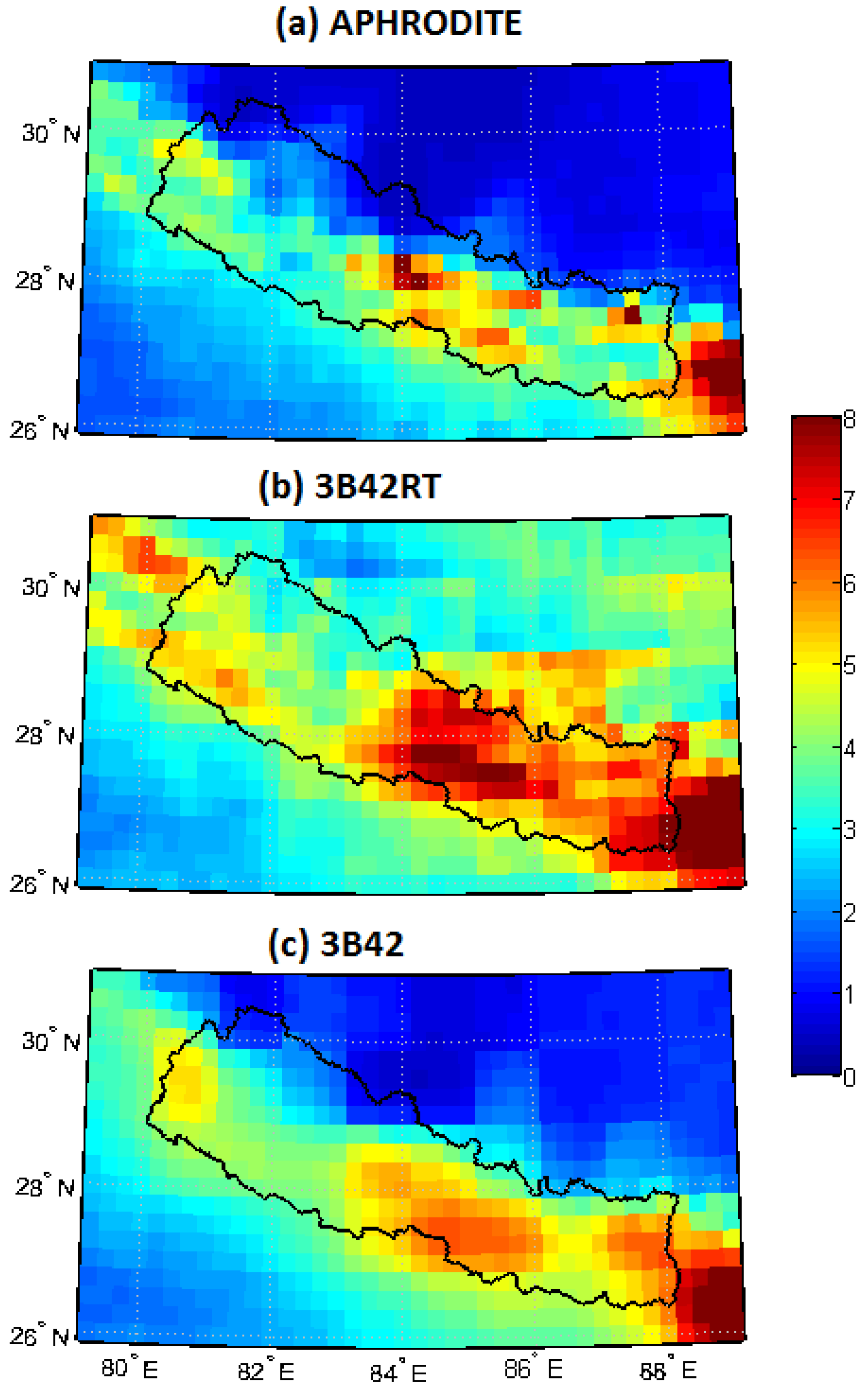
2.1. Satellite-Based Precipitation

TMPA Product 3B42 is released by the Goddard Space Flight Center of the National Aeronautics and Space Administration (NASA) [8]. Product 3B42 is a 3-hour precipitation product with a spatial resolution of 0.25°, available for the period since 1998, which incorporates microwave and infrared observations from multiple satellites including TRMM [9]. 3B42 is a retrospective research product that is generally updated with a lag of several months because it uses monthly rain gauge accumulations in order to correct the estimated precipitation field. Product 3B42RT [10] has the same spatial and temporal resolution as 3B42 but is processed in near real time, available since March 2000, with updated fields typically posted about 3 hours after the end of each 3-hour window. Both products are available globally over 50°S–50°N. While 3B42RT currently does not come with quantitative error estimates, it does include source information that distinguishes between pixels where the precipitation estimate is based on microwave sounders (more accurate) or only on infrared imagery (less accurate). Here, we consider the 3B42RT product because its near real time availability makes it more suitable than 3B42 for most hydrological applications, but also compare the two products to assess the extent to which after-the-fact calibration improves the correspondence with gauge-based precipitation. The product versions used were the most recent available as of early 2015, i.e., 3B42 Version 7, which has generally been found to improve on the older Version 6 [11,12,13]. Several studies have previously evaluated 3B42RT against ground measurements and other satellite-based products in different regions [14,15,16,17,18,19,20,21].

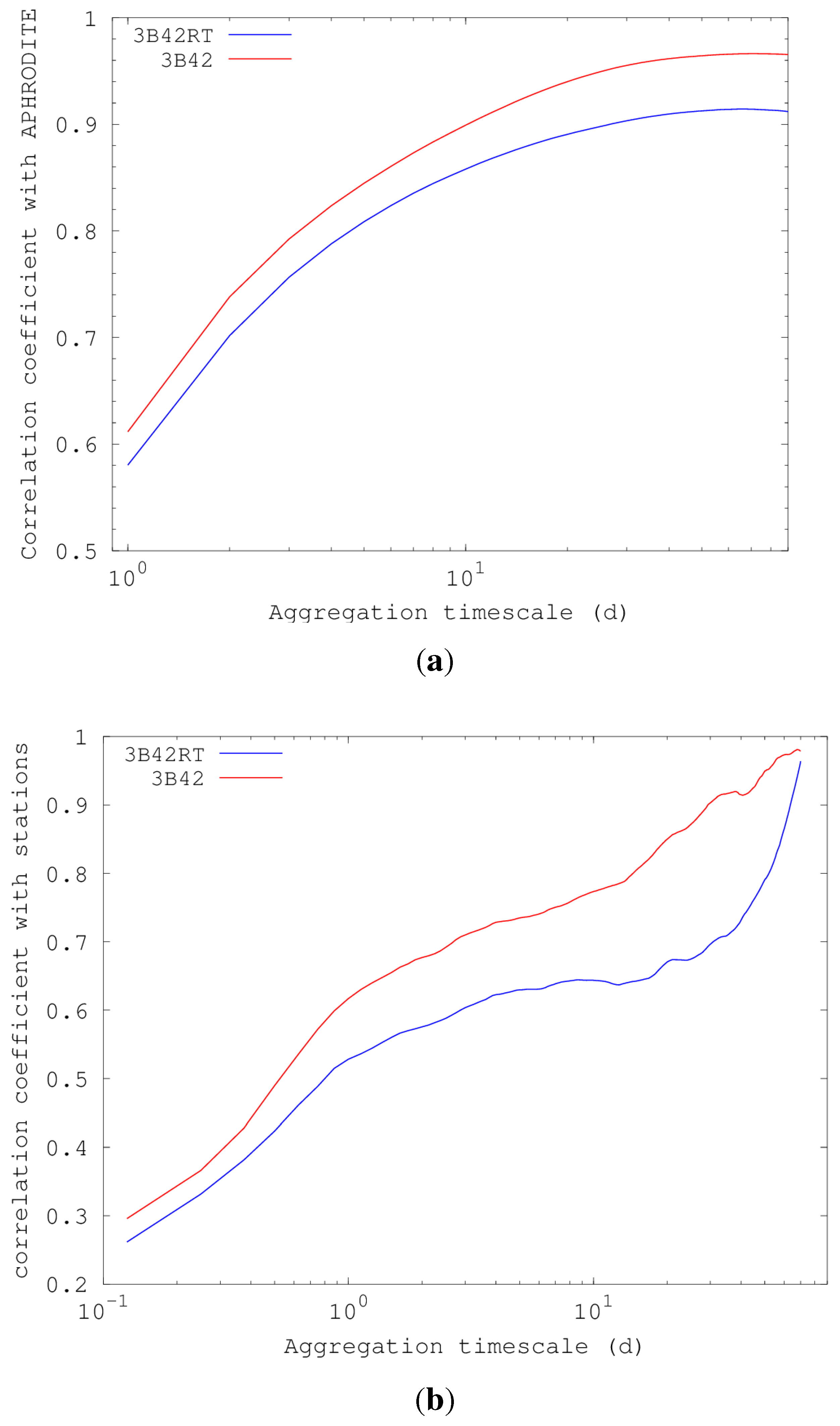
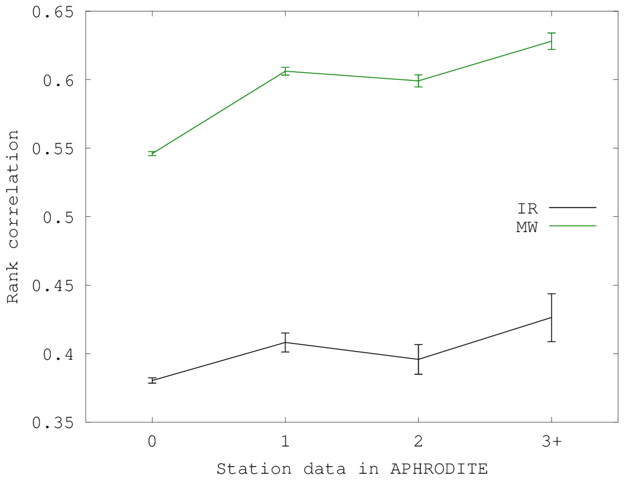
2.2. Gauge-Based Precipitation

Our primary “ground-truth” dataset in this study is from the Asian Precipitation—Highly Resolved Observational Data Integration Towards Evaluation of Water Resources (APHRODITE) project, which has produced a daily precipitation dataset over Asia based on an extensive compilation of rain gauge measurements [22], primarily station data obtained from national meteorological agencies, including Nepal's Department of Hydrology and Meteorology (DHM). Station data were interpolated using an algorithm that takes topography into account and uses climatology to estimate missing values. We used the APHRODITE V1101 monsoon Asia product at the best available resolution of 0.25°, which is available for 1951–2007. APHRODITE includes information on the percent of 0.05° cells in each pixel containing gauge data. Unless otherwise specified, we employed only 0.25° pixels for which this quantity was positive, i.e., which are directly based on at least some gauge measurements, in calibrating and comparing with the satellite products. The satellite products were aggregated to daily resolution for comparison with APHRODITE.

Note that one possible contributor for inconsistency between these data sets is that the days in the aggregated satellite products follow Universal Time (Greenwich Mean Time) while the reading times for the daily values recorded from gauges and used as the basis for the APHRODITE interpolation may vary [22]. However, in preliminary testing we found that shifting the satellite product aggregation window to allow for time zone and gauge reading time differences did not greatly change the correlations with APHRODITE daily values.

To characterize the performance of the TMPA satellite products in reproducing the precipitation diurnal cycle, we also compared them with precipitation measured at high temporal resolution at 3 automatic weather stations (AWSs) in Nepal installed by our team. These stations are located in farm fields representing different agro-ecological zones at (a) Baireni, Valtar in Dhading district, 27°47’0.45”N, 85°0’42.68”E (elevation of 550 m above sea level); (b) Tindobate, Jholpe in Syangja district, 27°58’17.48”N, 83°45’0.86”E (745 m); (c) Jayanagar, Gorusinge in Kapilvastu district, 27°40’41.38”N, 83°1’54.83”E (115 m). These stations record accumulated precipitation at 5 minute intervals and temperature and relative humidity at 15 minute intervals. The rain gauges use tipping buckets to measure precipitation at 0.2 mm resolution; the gauge models are TR-525S (manufactured by Texas Electronics, Inc., Dallas, Texas, USA) at the Dhading site and TB3 (Hydrological Services, Ltd., Sydney, NSW, Australia) at the other two sites. The gauges are not heated, since the site elevations are low enough that they do not experience snow. Data were available beginning June 2013 and ending September 2014 (Syangja and Kapilvastu) or December 2014 (Dhading).

3. Analysis Methods

3.1. General Approach

Probabilistic precipitation forecasts are common in the short-term synoptic context [23,24] and also for long-term seasonal prediction [25,26,27,28]. An ensemble of precipitation fields consistent with observations has been used to represent the uncertainty of radar-based precipitation estimates [29,30]. The uncertainty represented by such probability distributions or ensembles can be propagated to streamflow and water supply quantities using hydrological models [31]. Bellerby and Sun [32] is one study that adopted a probabilistic approach to precipitation retrieval from remote sensing, fitting gamma distributions to represent precipitation intensity probabilities at different measured cloud-top infrared brightness temperatures. Authors in [33] used a nonparametric (kernel density) approach to estimate 3-hourly precipitation occurrence and intensity probabilities over part of the United States conditional on retrievals from the satellite precipitation product CMORPH, but noted that sampling the resulting nonparametric probability distributions is not straightforward. Here, we model the probability distribution $p\left(x\right)$ of APHRODITE precipitation amount x by bringing together separate models for precipitation occurrence ($p(x>0)$) and precipitation intensity conditional on occurrence ($p\left(x\right|x>0)$). (An alternative approach would be to subsume both in one distribution that has a point mass at zero precipitation amount [34,35].) We use flexible parametric functional forms to facilitate fitting the conditional probability distributions to the observed precipitation amount data.

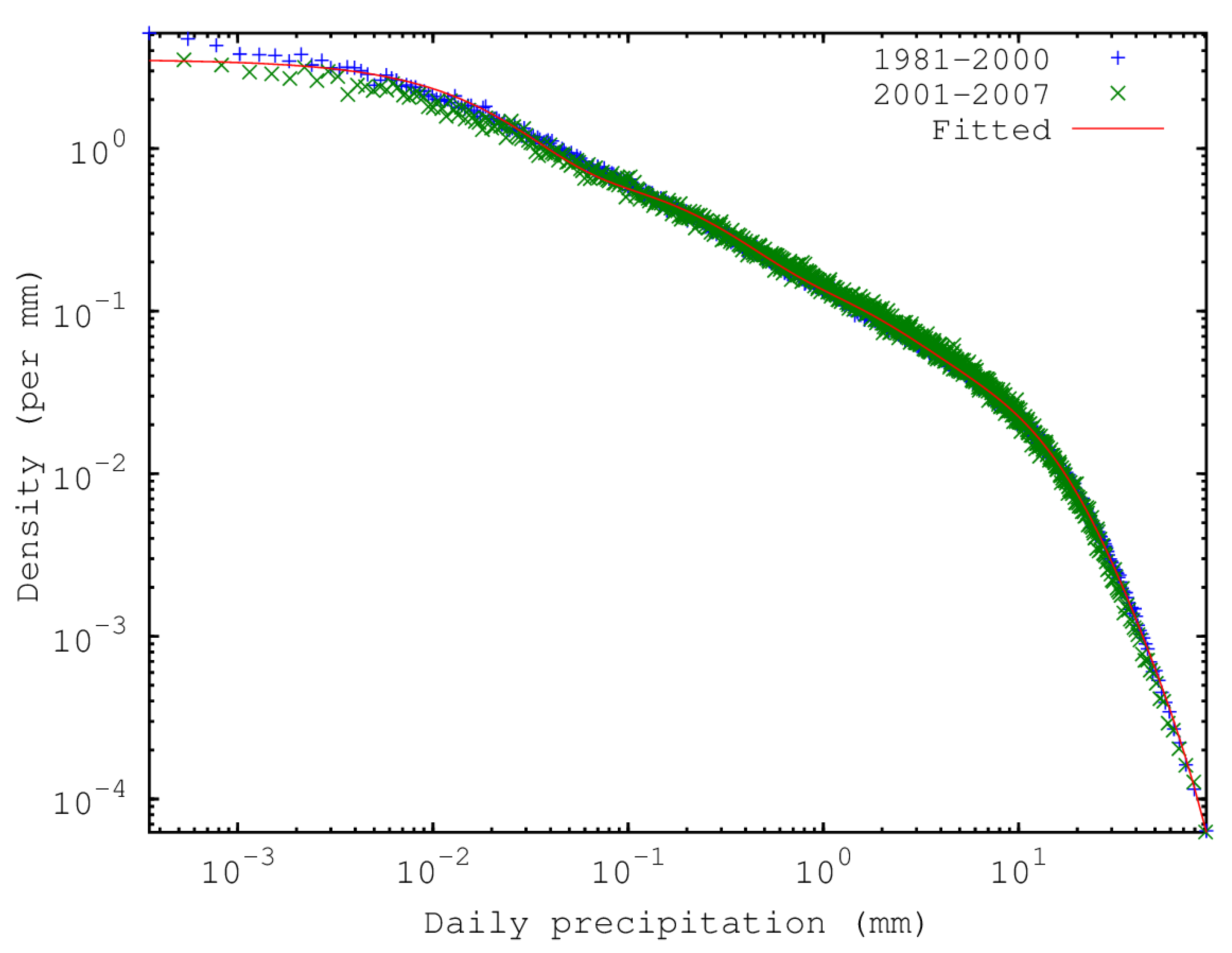
3.2. Precipitation Amount Modeling

For precipitation intensity, we assume a generalized linear model [36]

$$g\left(p\left(x\right|x>0)\right)\sim 𝒩(Z\beta ,{\sigma }^2)$$

(1)

where $𝒩$ denotes the normal distribution, Z is an $1\times l$ vector of predictor values, which can include climatological (observed spatial and seasonal variability), and 3B42RT terms, and β is a $k\times 1$ vector of coefficients. Values for β and the model standard deviation σ are determined by linear regression using the data from 2001–2007. Given this training data, standard statistical results show that $g\left(p\right(x|x>0))$ for unobserved data with a known set of predictor values is given by a t distribution [37]. Note that, for simplicity and to make use of all the available valid data, $\beta ,\sigma$ were fitted over the entire study domain and not for each grid point separately.

We compared 4 models, which differ in the predictor values considered: (a) no predictors (baseline probability distribution, which is the same for all times and places); (b) predictors based on the 3B42RT precipitation amount; (c) predictors based on spatial location and Fourier components of the seasonal cycle (climatology); (d) both 3B42RT and climatology predictors. For each of models (b)–(d), which predictors to retain out of a candidate set was decided using stepwise linear regression [38] as implemented in the stepwisefit function of the Statistics package in GNU Octave [39].

The transformation $g\left(p\right),$ which serves as the link function in the generalized linear model, is based on approximating the APHRODITE precipitation intensity probability density as a sum of exponential distributions, also known as a hyperexponential distribution:

$$p_H\left(x\right|x>0;\mathrm{a},\mathrm{b})=\sum _{i=1}^N{a}_i{e}^{-x/b_i}$$

(2)

with the component distributions arranged in order of scale, so that $0<b_1<b_2<...<b_N,$ and additional constraints $a_i>0,{\sum }_{i=1}^N{a}_i{b}_i=1.$ The coefficient values are chosen to maximize the likelihood of observed APHRODITE precipitation over 1981–2000, and the number of components N is chosen by applying the corrected Akaike information criterion [40,41] with the same data. (See Appendix for more details.)

A variety of probability distributions have been used to model daily precipitation intensity series, including the gamma distribution [42,43,44], a stretched exponential distribution based on the idea that precipitation intensity can be thought of as the product of three independent Gaussian variables representing mass flux, specific humidity, and precipitation efficiency [45], or a hybrid exponential and generalized Pareto distribution [46]. However, these distributions have few (2–3) adjustable parameters and cannot be made to fit daily precipitation series well over the entire range of precipitation intensity. By contrast, the hyperexponential distribution provides an analytically tractable approximation to the observed precipitation intensity distribution that can approximate well even long-tailed positive-valued distributions with monotone decreasing densities, such as those for queuing times [47]. wilks [48] previously considered a hyperexponential distribution with $N=2$ for precipitation intensity, and [49,50] use an exponential distribution (i.e., $N=1$) to model hourly precipitation intensity.

Given the fitted hyperexponential distribution, the link function is a normal quantile transform [51]:

$$g\left(x\right)=P_N^{\text{inv}}\left(P_H\left(x\right)\right)$$

(3)

where $P_H\left(x\right)={\int }_0^x{p}_H\left(u\right)du$ denotes the cumulative distribution function obtained by integrating the hyperexponential density function $p_H$ above, and $P_N^{\text{inv}}$ is the inverse of the standard normal cumulative distribution function.

The skill of the fitted probability distribution was evaluated using leave-one-month-out cross-validation with root mean square error (RMSE) and mean negative log likelihood (NLL) metrics. NLL is a particularly useful metric for probabilistic models because it evaluates not only the quality of the model's central estimate, as RMSE does, but also whether the model standard deviation is consistent with the model-observation spread [27]. The difference in NLL between an augmented model and a baseline can be interpreted as the information gain in bits (assuming base-2 logarithms are taken) from the data (such as 3B42RT) included in the augmented model. RMSE and NLL averages were computed over all APHRODITE rainy pixels ($x>0$) for the 2001–2007 period.

3.3. Precipitation Occurrence Modeling

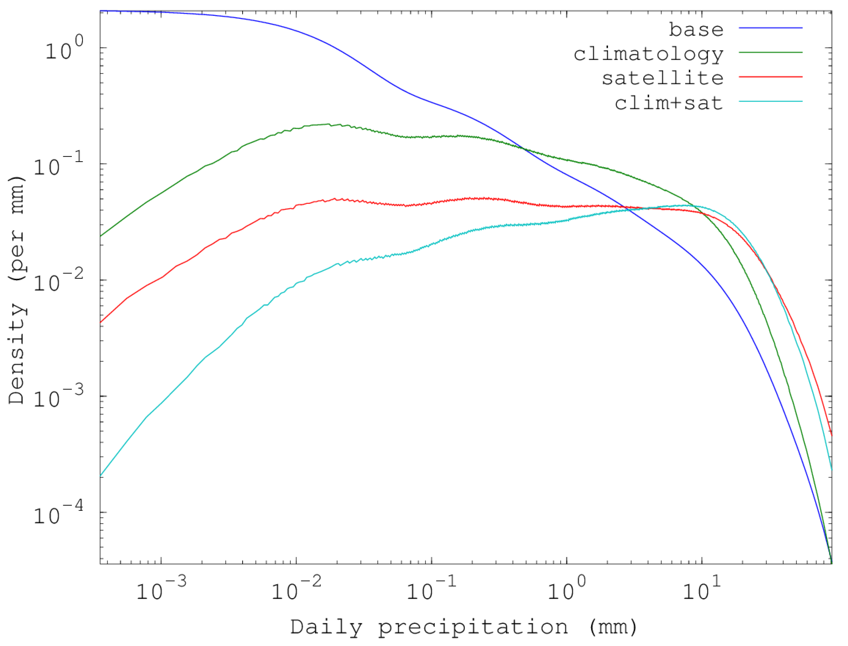
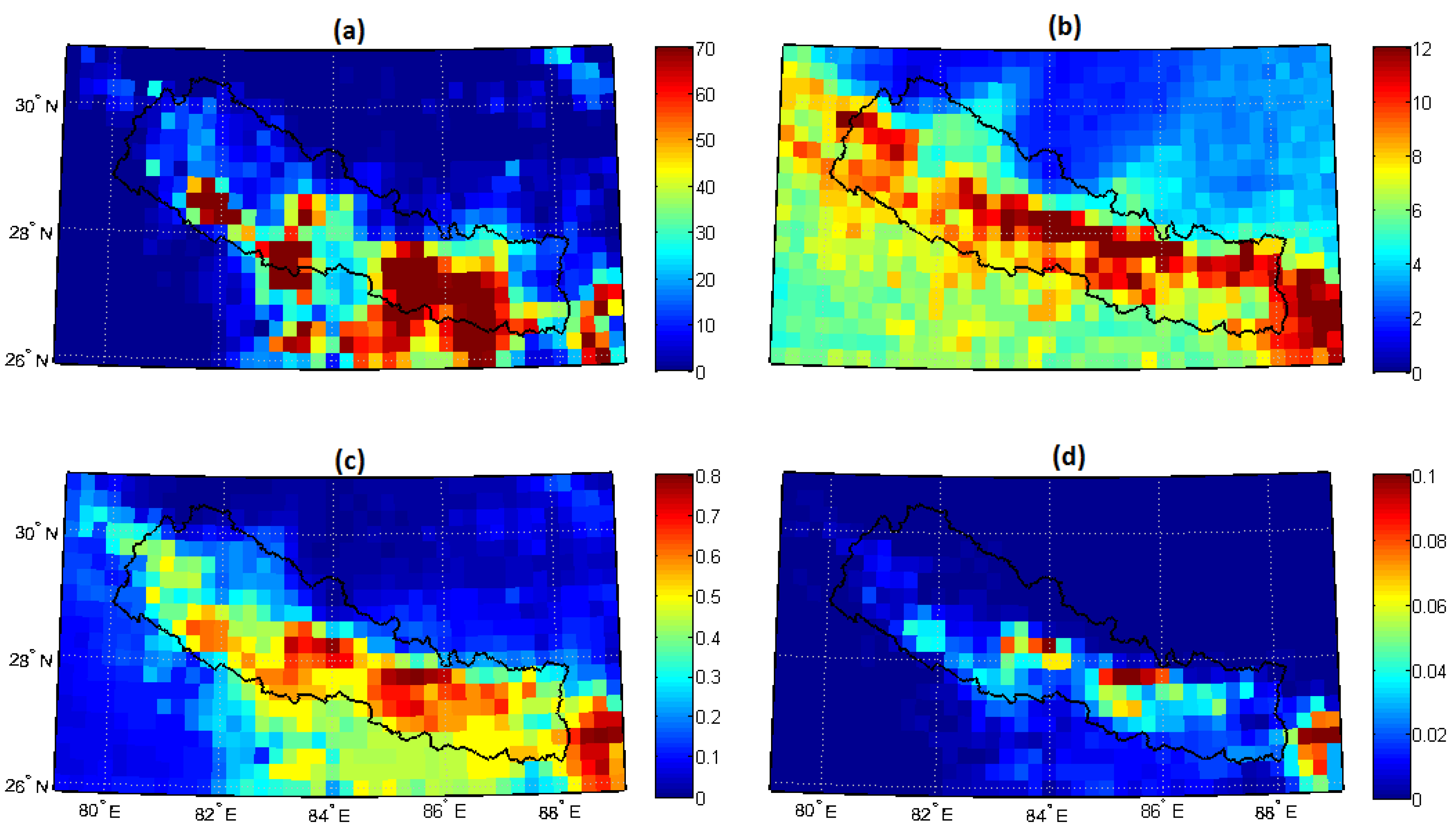
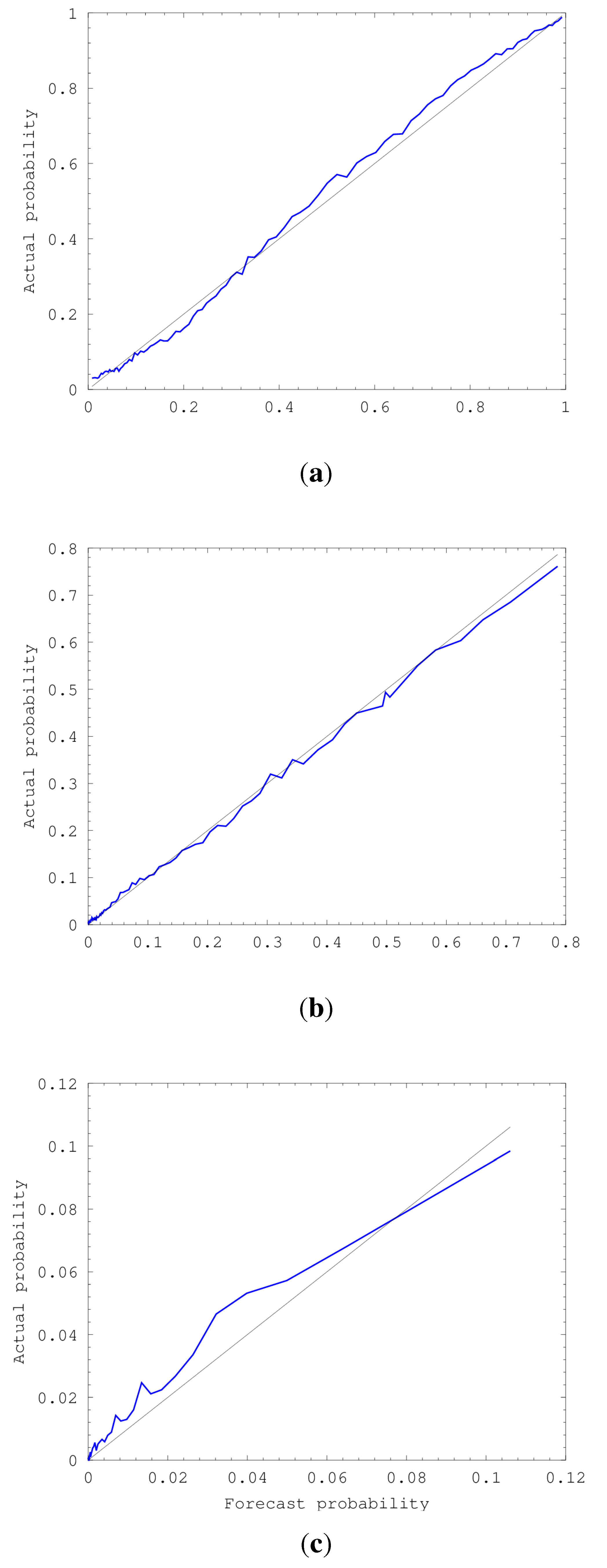
For precipitation occurrence, we assumed a logistic regression model, one form of a generalized linear model:

$$L\left(p\right(x>0\left)\right)=Z\gamma$$

(4)

where $L\left(p\right)$ denotes the logistic function $log\frac{p}{1-p},$ Z is a $1\times k$ vector of predictor values identical with that used in the precipitation amount model, and γ is a $k\times 1$ vector of coefficients. Given the predictors and APHRODITE data over 2001–2007, the coefficients γ were determined via maximum likelihood, using the trust region Newton method implemented in LIBLINEAR [52,53].

Skill measures for the precipitation occurrence model included both NLL and a probabilistic form of RMSE closely related to the popular Brier skill score [54,55], namely the square root of the average value of ${(p(x>0)-p_o)}^2,$ where the observation $p_o$ is equal to 1 if the day was rainy and 0 if not.

4. Results

We begin with a comparison of precipitation patterns between the satellite products (TMPA 3B42RT and 3B42) and ground-based products (APHRODITE and the AWSs). First, both satellite products have broadly similar regional spatial patterns of mean precipitation as APHRODITE when evaluated for the overlap period of 2001–2007 (Figure 1). 3B42 shows the benefits of retrospective calibration against rain gauges in a sharper precipitation gradient across the Himalayas that compares better with APHRODITE, whereas, as previously shown [20], 3B42RT overestimates precipitation over the Tibetan Plateau. On the other hand, 3B42RT better shows the double heavy-precipitation band just south of the Himalayas also seen in APHRODITE and missed by 3B42 because its calibration at 1° resolution imposes smoothing [6].

We next consider how the correspondence of satellite-derived with ground-based precipitation changes with timescale (Figure 2). We use rank correlation as an appropriate overall measure of correspondence, as this is less sensitive to the non-normal distribution of precipitation and to outlying values than Pearson product-moment correlation. The correlation coefficients of 3B42RT and 3B42 with APHRODITE are comparable on the daily timescale (0.58 and 0.61 respectively), and increase with aggregation time to 0.90 and 0.96 respectively at 30 days. Correlations with the AWSs behave similarly on the daily to monthly scales (coefficients of 0.53 and 0.62 at 1 day and 0.70 and 0.90 at 30 days—the somewhat lower correlations are expected given that we are comparing an individual station and not an interpolated product with the gridded satellite precipitation field), but show a sharp drop-off at shorter time scales than daily, down to 0.26 and 0.30 at 3 hours. On the other hand, the satellite products do roughly reproduce the pronounced precipitation diurnal cycle seen in the AWS observations, which features a maximum in early morning (local time) and a minimum in the afternoon (Figure 3). Previous studies suggest that the precipitation diurnal cycle in Nepal varies by season [56] and differs for precipitation occurrence versus amount [57], which we may consider in a future study.

At the daily timescale, 3B42RT was better correlated with APHRODITE when the satellite data quality was higher (as measured by more 3-hour periods with microwave precipitation rate determinations) and when the ground-based data quality is higher (as measured by more 0.05°squares with reporting gauges within the 0.25°pixel), with the satellite data quality having a more pronounced impact (Figure 4). This highlights the potential role of better observations in improving satellite-based precipitation products.

Figure 1. Mean precipitation (mm·d${}^{-1}$) over 2001–2007 from the gauge-based APHRODITE product and from the satellite-based 3B42RT and 3B42 products for Nepal and vicinity.

Figure 1. Mean precipitation (mm·d${}^{-1}$) over 2001–2007 from the gauge-based APHRODITE product and from the satellite-based 3B42RT and 3B42 products for Nepal and vicinity.

The regional APHRODITE daily precipitation amount distribution turned out to be fit very well by the sum of $N=5$ exponentials (Figure 5). The exponential function was a good basis for this probability distribution because the empirical probability density decreased for increasing precipitation amounts. (APHRODITE's spatial interpolation procedure favors showing light precipitation amounts rather than exactly zero precipitation, with about 60% nonzero daily precipitation amounts in the region.)

This baseline hyperexponential distribution was modified based on location, season, and 3B42RT precipitation to give spatiotemporally varying predictive distributions. An example of how this affects the base distribution is shown in Figure 6, illustrating a situation when both the monsoon season and the detection of heavy precipitation by 3B42RT implies a higher probability of heavy precipitation compared to the baseline. Probabilities for any precipitation level of interest being exceeded can be mapped over the entire region based on our combined climatology and satellite based model, and can be seen to reflect both climatological precipitation patterns and precipitation reported in 3B42RT (Figure 7).

Figure 2. Rank correlation of precipitation of the satellite-based 3B42RT and 3B42 products as a function of aggregation timescales: (a) Correlation with the gauge-based APHRODITE product for 2001–2007 over aggregation timescales from 1 to 90 days; (b) Correlation with automated weather stations for 2013–2014 over aggregation timescales from 3 hours to 90 days.

Figure 2. Rank correlation of precipitation of the satellite-based 3B42RT and 3B42 products as a function of aggregation timescales: (a) Correlation with the gauge-based APHRODITE product for 2001–2007 over aggregation timescales from 1 to 90 days; (b) Correlation with automated weather stations for 2013–2014 over aggregation timescales from 3 hours to 90 days.

Figure 3. Mean precipitation diurnal cycle, 2013–2014, averaged across 3 stations in Nepal (5-minute values and a Fourier series smoothed fit are shown) and for satellite products with 3-hour resolution subsampled at the same grid points. Nepal Standard Time is 5:45 hours ahead of Universal Time.

Figure 3. Mean precipitation diurnal cycle, 2013–2014, averaged across 3 stations in Nepal (5-minute values and a Fourier series smoothed fit are shown) and for satellite products with 3-hour resolution subsampled at the same grid points. Nepal Standard Time is 5:45 hours ahead of Universal Time.

Figure 4. Rank correlation of daily precipitation between the satellite-based 3B42RT product and APHRODITE as a function of both station data coverage (expressed as the number of 0.05°subcells in a 0.25°grid cell with precipitation gauges) and satellite data coverage (availability of higher-quality microwave (MW) sounder precipitation estimates for at least 4 of the daily 3-hour windows versus only lower-quality estimates based on infrared (IR) imagery). Error bars are 95% confidence intervals for the correlation coefficients.

Figure 4. Rank correlation of daily precipitation between the satellite-based 3B42RT product and APHRODITE as a function of both station data coverage (expressed as the number of 0.05°subcells in a 0.25°grid cell with precipitation gauges) and satellite data coverage (availability of higher-quality microwave (MW) sounder precipitation estimates for at least 4 of the daily 3-hour windows versus only lower-quality estimates based on infrared (IR) imagery). Error bars are 95% confidence intervals for the correlation coefficients.

Figure 5. Empirical probability density for APHRODITE daily precipitation amount at the 0.25°grid scale (conditional on occurrence) for the region 26°–31°N, 79°–89°E and for two time periods, compared with a hyperexponential distribution fit only to the 1981–2000 data.

Figure 5. Empirical probability density for APHRODITE daily precipitation amount at the 0.25°grid scale (conditional on occurrence) for the region 26°–31°N, 79°–89°E and for two time periods, compared with a hyperexponential distribution fit only to the 1981–2000 data.

Figure 6. Example probability density functions for daily precipitation amount at the grid point containing Kathmandu, Nepal (27.7°N, 85.3°E) for a heavy-rainfall monsoon day (2 September 2013): background PDF, climatology PDF taking into account location and season, and probabilities that incorporate data from the satellite precipitation product 3B42RT.

Figure 6. Example probability density functions for daily precipitation amount at the grid point containing Kathmandu, Nepal (27.7°N, 85.3°E) for a heavy-rainfall monsoon day (2 September 2013): background PDF, climatology PDF taking into account location and season, and probabilities that incorporate data from the satellite precipitation product 3B42RT.

Figure 7. Example maps of regional precipitation for 2 September 2013: (a) 3B42RT amount (mm); (b) climatological mean (mm); (c) probability of precipitation > 10 mm based on combined climatology + satellite model; (d) probability of precipitation > 50 mm.

Figure 7. Example maps of regional precipitation for 2 September 2013: (a) 3B42RT amount (mm); (b) climatological mean (mm); (c) probability of precipitation > 10 mm based on combined climatology + satellite model; (d) probability of precipitation > 50 mm.

Table 1. Skill measures for probabilistic daily precipitation estimates relative to APHRODITE values averaged over Nepal and vicinity, 2001–2007. The models are B = baseline (same probability distribution for all locations and days), S = satellite (incorporates precipitation from 3B42RT), C = climatology (incorporates past patterns of precipitation location and seasonality), Comb = combined (both satellite and climatology predictors). NLL = negative log likelihood, RMSE = root mean square error. RMSE is in transformed precipitation units, while NLL is in bits. Smaller values denote more skill. Precipitation amount skill measures are averaged only over cases with nonzero precipitation in APHRODITE.

	B	S	C	Comb
Precipitation amount:
RMSE	0.957	0.839	0.776	0.742
NLL	2.064	1.875	1.759	1.715
Precipitation occurrence:
RMSE	0.486	0.433	0.382	0.364
NLL	0.961	0.776	0.641	0.588

Table 1. Skill measures for probabilistic daily precipitation estimates relative to APHRODITE values averaged over Nepal and vicinity, 2001–2007. The models are B = baseline (same probability distribution for all locations and days), S = satellite (incorporates precipitation from 3B42RT), C = climatology (incorporates past patterns of precipitation location and seasonality), Comb = combined (both satellite and climatology predictors). NLL = negative log likelihood, RMSE = root mean square error. RMSE is in transformed precipitation units, while NLL is in bits. Smaller values denote more skill. Precipitation amount skill measures are averaged only over cases with nonzero precipitation in APHRODITE.

	B	S	C	Comb
Precipitation amount:
RMSE	0.957	0.839	0.776	0.742
NLL	2.064	1.875	1.759	1.715
Precipitation occurrence:
RMSE	0.486	0.433	0.382	0.364
NLL	0.961	0.776	0.641	0.588

Figure 8. Frequency of precipitation above different threshold values ((a) 1; (b) 10; (c) 50 mm/day) as a function of modeled probability (combined satellite and climatology model). 1-1 lines indicating an ideally calibrated model are also shown.

Figure 8. Frequency of precipitation above different threshold values ((a) 1; (b) 10; (c) 50 mm/day) as a function of modeled probability (combined satellite and climatology model). 1-1 lines indicating an ideally calibrated model are also shown.

Skill measures for the different probabilistic models show that both the climatology and 3B42RT measures yield improvements over the baseline probability distribution, and their combination yields the best performing models for both precipitation occurrence and precipitation amount (Table 1). Note that while the satellite product yields some 0.19 bits of information gain over baseline for precipitation amount (S versus B NLL in Table 1), satellite plus climatology only outperforms climatology by 0.04 bits (Comb versus C). Results for the other skill measures show the same trend, presumably because much of the correlation of the satellite product with APHRODITE reflects spatial and mean seasonal patterns of variability that can be captured in climatology, whereas it does not offer as much useful information on interannual variability [6].

Well calibrated probabilities are an important feature for a probabilistic monitoring model, and the models developed here indeed generally give probabilities that match the observed (APHRODITE) frequency of occurrence for precipitation over a wide range of threshold values and model probabilities (Figure 8), despite their linearity in transformed precipitation amount.

5. Discussion and Conclusions

Likely the most useful extension of the model offered here would be adding other sources of information available in near real time. These include numerical weather prediction model output fields, regional circulation pattern variables and global modes of variability that affect precipitation expectation [58,59,60], and any ground-based radar or weather stations available in near real time. Improvements in the availability and quality of past ground-based precipitation datasets for model calibration (such as extending APHRODITE past 2007) would also be expected to improve precipitation retrievals. While most precipitation in the region occurs in summertime as rain, special treatment of snow may be explored to improve high-altitude winter precipitation retrievals [61] considering that the current algorithms for converting satellite sensor values to precipitation rates have been developed primarily for liquid precipitation and have been shown to underestimate snowfall water equivalent [62].

Including spatial and temporal correlations is another possible direction for extension. How to efficiently specify mutivariate probability distributions in highly non-normal quantities such as daily precipitation amounts is an active area of research [29,46,63,64].

Our work here presents a comprehensive approach to constructing a probabilistic model of precipitation given an imperfect, deterministic satellite precipitation product without explicit error information and ground-based observations from past years. We anticipate that this method could be adapted to different regions where near-real-time precipitation observations are scarce.

References

1. Serrat-Capdevila, A.; Valdes, J.B.; Stakhiv, E.Z. Water management applications for satellite precipitation products: Synthesis and recommendations. J. Am. Water Resour. Assoc. 2014, 50, 509–525. [Google Scholar] [CrossRef]
2. Chalise, S.B.; Shrestha, M.L.; Thapa, K.B.; Shrestha, B.R.; Bajracharya, B. Climate and Hydrological Atlas of Nepal; International Center for Integrated Mountain Development: Kathmandu, New Zealand, 1996. [Google Scholar]
3. Panthi, J.; Dahal, P.; Shrestha, M.L.; Aryal, S.; Krakauer, N.Y.; Pradhanang, S.M.; Lakhankar, T.; Jha, A.K.; Sharma, M.; Karki, R. Spatial and Temporal Variability of Rainfall in the Gandaki River Basin of Nepal Himalaya. Climate 2015, 3, 210–226. [Google Scholar] [CrossRef]
4. Dhakal, C.K.; Regmi, P.P.; Dhakal, I.P.; Khanal, B.; Bhatta, U.K. Livelihood Vulnerability to Climate Change based on Agro Ecological Regions of Nepal. Glob. J. Sci. Front. Res. 2013, 13, 47–53. [Google Scholar]
5. Pradhanang, U.B.; Pradhanang, S.M.; Sthapit, A.; Krakauer, N.Y.; Jha, A.; Lakhankar, T. National livestock policy of Nepal: Needs and opportunities. Agriculture 2015, 5, 103–131. [Google Scholar] [CrossRef]
6. Krakauer, N.Y.; Pradhanang, S.M.; Lakhankar, T.; Jha, A.K. Evaluating satellite products for precipitation estimation in mountain regions: A case study for Nepal. Remote Sens. 2013, 5, 4107–4123. [Google Scholar] [CrossRef]
7. Hossain, F.; Huffman, G.J. Investigating error metrics for satellite rainfall data at hydrologically relevant scales. J. Hydrometeorol. 2008, 9, 563–575. [Google Scholar] [CrossRef]
8. Huffman, G.J.; Bolvin, D.T.; Nelkin, E.J.; Wolff, D.B.; Adler, R.F.; Gu, G.; Hong, Y.; Bowman, K.P.; Stocker, E.F. The TRMM Multisatellite Precipitation Analysis (TMPA): Quasi-global, multiyear, combined-sensor precipitation estimates at fine scales. J. Hydrometeorol. 2007, 8, 38–55. [Google Scholar] [CrossRef]
9. Kummerow, C.; Barnes, W.; Kozu, T.; Shiue, J.; Simpson, J. The Tropical Rainfall Measuring Mission (TRMM) sensor package. J. Atmos. Ocean. Technol. 1998, 15, 809–817. [Google Scholar] [CrossRef]
10. Huffman, G.; Adler, R.; Bolvin, D.; Nelkin, E. The TRMM multi-satellite precipitation analysis (TMPA). In Satellite Rainfall Applications For Surface Hydrology; Springer: Berlin, Germany, 2010; pp. 3–22. [Google Scholar]
11. Chen, S.; Hong, Y.; Cao, Q.; Gourley, J.J.; Kirstetter, P.E.; Yong, B.; Tian, Y.; Zhang, Z.; Shen, Y.; Hu, J.; Hardy, J. Similarity and difference of the two successive V6 and V7 TRMM multisatellite precipitation analysis performance over China. J. Geophys. Res. Atmosp. 2013, 118, 13060–13074. [Google Scholar] [CrossRef]
12. Qiao, L.; Hong, Y.; Chen, S.; Zou, C.B.; Gourley, J.J.; Yong, B. Performance assessment of successive Version 6 and Version 7 TMPA products over the climate-transitional zone in the southern Great Plains, USA. J. Hydrol. 2014, 513, 446–456. [Google Scholar] [CrossRef]
13. Chen, S.; Hong, Y.; Gourley, J.J.; Huffman, G.J.; Tian, Y.; Cao, Q.; Yong, B.; Kirstetter, P.E.; Hu, J.; Hardy, J.; Li, Z.; Khan, S.I.; Xue, X. Evaluation of the successive V6 and V7 TRMM multisatellite precipitation analysis over the Continental United States. Water Resour. Res. 2013, 49, 8174–8186. [Google Scholar] [CrossRef]
14. Gourley, J.J.; Hong, Y.; Flamig, Z.L.; Li, L.; Wang, J. Intercomparison of rainfall estimates from radar, satellite, gauge, and combinations for a season of record rainfall. J. Appl. Meteorol. Climatol. 2010, 49, 437–452. [Google Scholar] [CrossRef]
15. Hirpa, F.A.; Gebremichael, M.; Hopson, T. Evaluation of high-resolution satellite precipitation products over very complex terrain in Ethiopia. J. Appl. Meteorol. Climatol. 2010, 49, 1044–1051. [Google Scholar] [CrossRef]
16. Yong, B.; Chen, B.; Gourley, J.J.; Ren, L.; Hong, Y.; Chen, X.; Wang, W.; Chen, S.; Gong, L. Intercomparison of the Version-6 and Version-7 TMPA precipitation products over high and low latitudes basins with independent gauge networks: Is the newer version better in both real-time and post-real-time analysis for water resources and hydrologic extremes? J. Hydrol. 2014, 508, 77–87. [Google Scholar]
17. Moazami, S.; Golian, S.; Hong, Y.; Sheng, C.; Kavianpour, M.R. Comprehensive evaluation of four high-resolution satellite precipitation products over diverse climate conditions in Iran. Hydrol. Sci. J. 2014. [Google Scholar] [CrossRef]
18. Huang, Y.; Chen, S.; Cao, Q.; Hong, Y.; Wu, B.; Huang, M.; Qiao, L.; Zhang, Z.; Li, Z.; Li, W.a. Evaluation of version-7 TRMM multi-satellite precipitation analysis product during the Beijing extreme heavy rainfall event of 21 July 2012. Water 2014, 6, 32–44. [Google Scholar] [CrossRef]
19. Liu, Z. Comparison of precipitation estimates between Version 7 3-hourly TRMM Multi-Satellite Precipitation Analysis (TMPA) near-real-time and research products. Atmos. Res. 2015, 153, 119–133. [Google Scholar] [CrossRef]
20. Tong, K.; Su, F.; Yang, D.; Hao, Z. Evaluation of satellite precipitation retrievals and their potential utilities in hydrologic modeling over the Tibetan Plateau. J. Hydrol. 2014, 519A, 423–437. [Google Scholar] [CrossRef]
21. Mantas, V.M.; Liu, Z.; Caro, C.; Pereira, A.J.S.C. Validation of TRMM multi-satellite precipitation analysis (TMPA) products in the Peruvian Andes. Atmos. Res. 2015, in press. [Google Scholar] [CrossRef]
22. Yatagai, A.; Kamiguchi, K.; Arakawa, O.; Hamada, A.; Yasutomi, N.; Kitoh, A. APHRODITE: Constructing a long-term daily gridded precipitation dataset for Asia based on a dense network of rain gauges. Bull. Am. Meteorol. Soc. 2012, 93, 1401–1415. [Google Scholar] [CrossRef]
23. Theis, S.E.; Hense, A.; Damrath, U. Probabilistic precipitation forecasts from a deterministic model: A pragmatic approach. Meteorol. Appl. 2005, 12, 257–268. [Google Scholar] [CrossRef]
24. Hamill, T.M. Verification of TIGGE Multimodel and ECMWF Reforecast-Calibrated Probabilistic Precipitation Forecasts over the Contiguous United States. Mon. Weather Rev. 2012, 140, 2232–2252. [Google Scholar] [CrossRef]
25. Mason, S.J.; Goddard, L. Probabilistic precipitation anomalies associated with ENSO. Bull. Am. Meteorol. Soc. 2001, 82, 619–638. [Google Scholar] [CrossRef]
26. Barnston, A.G.; Mason, S.J. Evaluation of IRI’s seasonal climate forecasts for the extreme 15% tails. Weather Forecast. 2011, 26, 545–554. [Google Scholar] [CrossRef]
27. Krakauer, N.Y.; Grossberg, M.D.; Gladkova, I.; Aizenman, H. Information content of seasonal forecasts in a changing climate. Adv. Meteorol. 2013, 2013, 480210. [Google Scholar] [CrossRef]
28. Luo, L.; Tang, W.; Lin, Z.; Wood, E.F. Evaluation of summer temperature and precipitation predictions from NCEP CFSv2 retrospective forecast over China. Clim. Dyn. 2013, 41, 2213–2230. [Google Scholar] [CrossRef]
29. Germann, U.; Berenguer, M.; Sempere-Torres, D.; Zappa, M. REAL–Ensemble radar precipitation estimation for hydrology in a mountainous region. Q. J. R. Meteorol. Soc. 2009, 135, 445–456. [Google Scholar] [CrossRef] [Green Version]
30. Tesfagiorgis, K.; Mahani, S.E.; Krakauer, N.Y.; Khanbilvardi, R. Bias correction of satellite rainfall estimates using a radar-gauge product – a case study in Oklahoma (USA). Hydrol. Earth Syst. Sci. 2011, 15, 2631–2647. [Google Scholar] [CrossRef]
31. Schaake, J.; Demargne, J.; Hartman, R.; Mullusky, M.; Welles, E.; Wu, L.; Herr, H.; Fan, X.; Seo, D.J. Precipitation and temperature ensemble forecasts from single-value forecasts. Hydrol. Earth Syst. Sci. Discuss. 2007, 4, 655–717. [Google Scholar] [CrossRef]
32. Bellerby, T.J.; Sun, J. Probabilistic and ensemble representations of the uncertainty in an IR/microwave satellite precipitation product. J. Hydrometeorol. 2005, 6, 1032–1044. [Google Scholar] [CrossRef]
33. Gebremichael, M.; Liao, G.Y.; Yan, J. Nonparametric error model for a high resolution satellite rainfall product. Water Resour. Res. 2011, 47, W07504. [Google Scholar] [CrossRef]
34. Dunn, P.K. Occurrence and quantity of precipitation can be modelled simultaneously. Int. J. Climatol. 2004, 24, 1231–1239. [Google Scholar] [CrossRef] [Green Version]
35. Hasan, M.M.; Dunn, P.K. Two Tweedie distributions that are near-optimal for modelling monthly rainfall in Australia. Int. J. Climatol. 2011, 31, 1389–1397. [Google Scholar] [CrossRef]
36. Chandler, R.E. On the use of generalized linear models for interpreting climate variability. Environmetrics 2005, 16, 699–715. [Google Scholar] [CrossRef]
37. Krakauer, N.Y.; Devineni, N. Up-to-date probabilistic temperature climatologies. Environ. Res. Lett. 2015, 10, 024014. [Google Scholar] [CrossRef]
38. Draper, N.R.; Smith, H. Applied Regression Analysis; Wiley: New York, NY, USA, 1966. [Google Scholar]
39. Eaton, J.W. GNU Octave and reproducible research. J. Process Control 2012, 22, 1433–1438. [Google Scholar] [CrossRef]
40. Hurvich, C.M.; Simonoff, J.S.; Tsai, C.L. Smoothing parameter selection in nonparametric regression using an improved Akaike information criterion. J. R. Stat. Soc. 1998, 60B, 271–293. [Google Scholar] [CrossRef]
41. Krakauer, N.Y.; Krakauer, J.C. A new body shape index predicts mortality hazard independently of body mass index. PLoS ONE 2012, 7, e39504. [Google Scholar] [CrossRef] [PubMed]
42. Stern, R.D. The calculation of probability distributions for models of daily precipitation. Arch. Meteorol. Geophys. Bioklimatol. Serie B 1980, 28, 137–147. [Google Scholar] [CrossRef]
43. Groisman, P.Y.; Karl, T.R.; Easterling, D.R.; Knight, R.W.; Jamason, P.F.; Hennessy, K.J.; Suppiah, R.; Page, C.M.; Wibig, J.; Fortuniak, K.; Razuvaev, V.N.; Douglas, A.; Førland, E.; Zhai, P.M. Changes in the probability of heavy precipitation: important indicators of climatic change. Clim. Chang. 1999, 42, 243–283. [Google Scholar] [CrossRef]
44. Semenov, V.; Bengtsson, L. Secular trends in daily precipitation characteristics: Greenhouse gas simulation with a coupled AOGCM. Clim. Dyn. 2002, 19, 123–140. [Google Scholar]
45. Wilson, P.S.; Toumi, R. A fundamental probability distribution for heavy rainfall. Geophys. Res. Lett. 2005, 32, 022465. [Google Scholar] [CrossRef]
46. Li, C.; Singh, V.P.; Mishra, A.K. A bivariate mixed distribution with a heavy-tailed component and its application to single-site daily rainfall simulation. Water Resour. Res. 2013, 49, 767–789. [Google Scholar] [CrossRef]
47. Feldmann, A.; Whitt, W. Fitting mixtures of exponentials to long-tail distributions to analyze network performance models. In Proceedings of the Sixteenth IEEE Annual Joint Conference of the Computer and Communications Societies, Kobe, Japan, 7–12 April 1997.
48. Wilks, D.S. Interannual variability and extreme-value characteristics of several stochastic daily precipitation models. Agric. For. Meteorol. 1999, 93, 153–169. [Google Scholar] [CrossRef]
49. Shamir, E.; Wang, J.; Georgakakos, K.P. Probabilistic streamflow generation model for data sparse arid watersheds. J. Am. Water Resour. Assoc. 2007, 43, 1142–1154. [Google Scholar] [CrossRef]
50. Shamir, E.; Megdal, S.B.; Carrillo, C.; Castro, C.L.; Chang, H.I.; Chief, K.; Corkhill, F.E.; Eden, S.; Georgakakos, K.P.; Nelson, K.M.; Prietto, J. Climate change and water resourcesmanagement in the Upper Santa Cruz River, Arizona. J. Hydrol. 2015, 521, 18–33. [Google Scholar] [CrossRef]
51. Bogner, K.; Pappenberger, F.; Cloke, H.L. Technical Note: The normal quantile transformation and its application in a flood forecasting system. Hydrol. Earth Syst. Sci. 2012, 16, 1085–1094. [Google Scholar] [CrossRef]
52. Lin, C.J.; Weng, R.C.; Keerthi, S.S. Trust region Newton method for large-scale logistic regression. J. Mach. Learn. Res. 2008, 9, 627–650. [Google Scholar]
53. Fan, R.E.; Chang, K.W.; Hsieh, C.J.; Wang, X.R.; Lin, C.J. LIBLINEAR: A library for large linear classification. J. Mach. Learn. Res. 2008, 9, 1871–1874. [Google Scholar]
54. Roulston, M.S.; Smith, L.A. Evaluating probabilistic forecasts using information theory. Mon. Weather Rev. 2002, 130, 1653–1660. [Google Scholar] [CrossRef]
55. Benedetti, R. Scoring rules for forecast verification. Mon. Weather Rev. 2010, 138, 203–211. [Google Scholar] [CrossRef]
56. Shrestha, D.; Deshar, R. Diurnal variation of pre-monsoon and monsoon rainfall over Nepal. In Proceedings of the 2014 Seminar on Water & Energy, Kathmandu, Nepal, 24 March 2014.
57. Bhatt, B.C.; Nakamura, K. Characteristics of monsoon rainfall around the Himalayas revealed by TRMM precipitation radar. Mon. Weather Rev. 2005, 133, 149–165. [Google Scholar] [CrossRef]
58. Bogardi, I.; Matyasovszky, I.; Bardossy, A.; Duckstein, L. Application of a space-time stochastic model for daily precipitation using atmospheric circulation patterns. J. Geophys. Res. 1993, 98, 16653–16667. [Google Scholar] [CrossRef]
59. Morin, J.; Block, P.; Rajagopalan, B.; Clark, M. Identification of large scale climate patterns affecting snow variability in the eastern United States. Int. J. Climatol. 2007, 28, 315–328. [Google Scholar] [CrossRef]
60. Kenyon, J.; Hegerl, G.C. Influence of modes of climate variability on global precipitation extremes. J. Clim. 2010, 23, 6248–6262. [Google Scholar] [CrossRef]
61. Lang, T.J.; Barros, A.P. Winter storms in the central Himalayas. J. Meteorol. Soc. Jpn. 2004, 82, 829–844. [Google Scholar] [CrossRef]
62. Anders, A.M.; Roe, G.H.; Hallet, B.; Montgomery, D.R.; Finnegan, N.J.; Putkonen, J. Spatial patterns of precipitation and topography in the Himalaya. Geol. Soc. Am. Special Papers 2006, 398, 39–53. [Google Scholar]
63. Mirakbari, M.; Ganji, A.; Fallah, S. Regional bivariate frequency analysis of meteorological droughts. J. Hydrol. Eng. 2010, 15, 985–1000. [Google Scholar] [CrossRef]
64. Peleg, N.; Shamir, E.; Georgakakos, K.P.; Morin, E. A framework for assessing hydrological regime sensitivity to climate change in a convective rainfall environment: a case study of two medium-sized eastern Mediterranean catchments, Israel. Hydrol. Earth Syst. Sci. 2015, 19, 567–581. [Google Scholar] [CrossRef]
65. Nelder, J.A.; Mead, R. A simplex method for function minimization. Comput. J. 1965, 7, 308–313. [Google Scholar] [CrossRef]
66. Asmussen, S.; Nerman, O.; Olsson, M. Fitting phase-type distributions via the EM algorithm. Scan. J. Stat. 1996, 23, 419–441. [Google Scholar]
67. Horváth, A.; Telek, M. PhFit: A general phase-type fitting tool. In Computer Performance Evaluation: Modelling Techniques and Tools; Field, T., Harrison, P., Bradley, J., Harder, U., Eds.; Springer: Berlin, Germany, 2002; pp. 82–91. [Google Scholar]
68. Gleser, L.J. The gamma distribution as a mixture of exponential distributions. Am. Stat. 1989, 43, 115–117. [Google Scholar]
69. Botta, R.F.; Harris, C.M. Approximation with generalized hyperexponential distributions: Weak convergence results. Queueing Syst. 1986, 1, 169–190. [Google Scholar] [CrossRef]
70. Riska, A.; Diev, V.; Smirni, E. An EM-based technique for approximating long-tailed data sets with PH distributions. Perform. Eval. 2004, 55, 147–164. [Google Scholar] [CrossRef]