
Statistical Seasonal Rainfall Forecast in the Neuquén River Basin (Comahue Region, Argentina)

Abstract
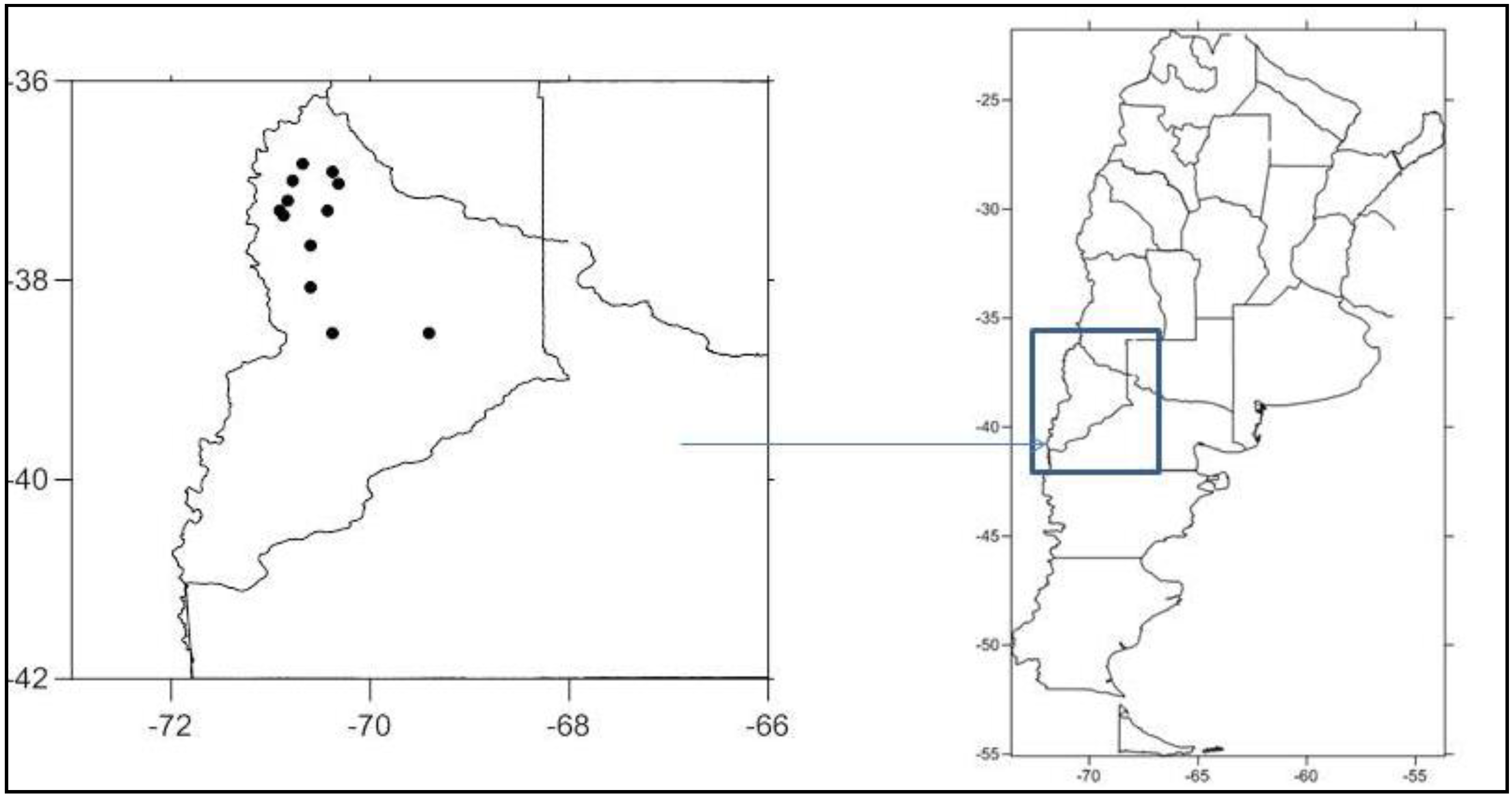
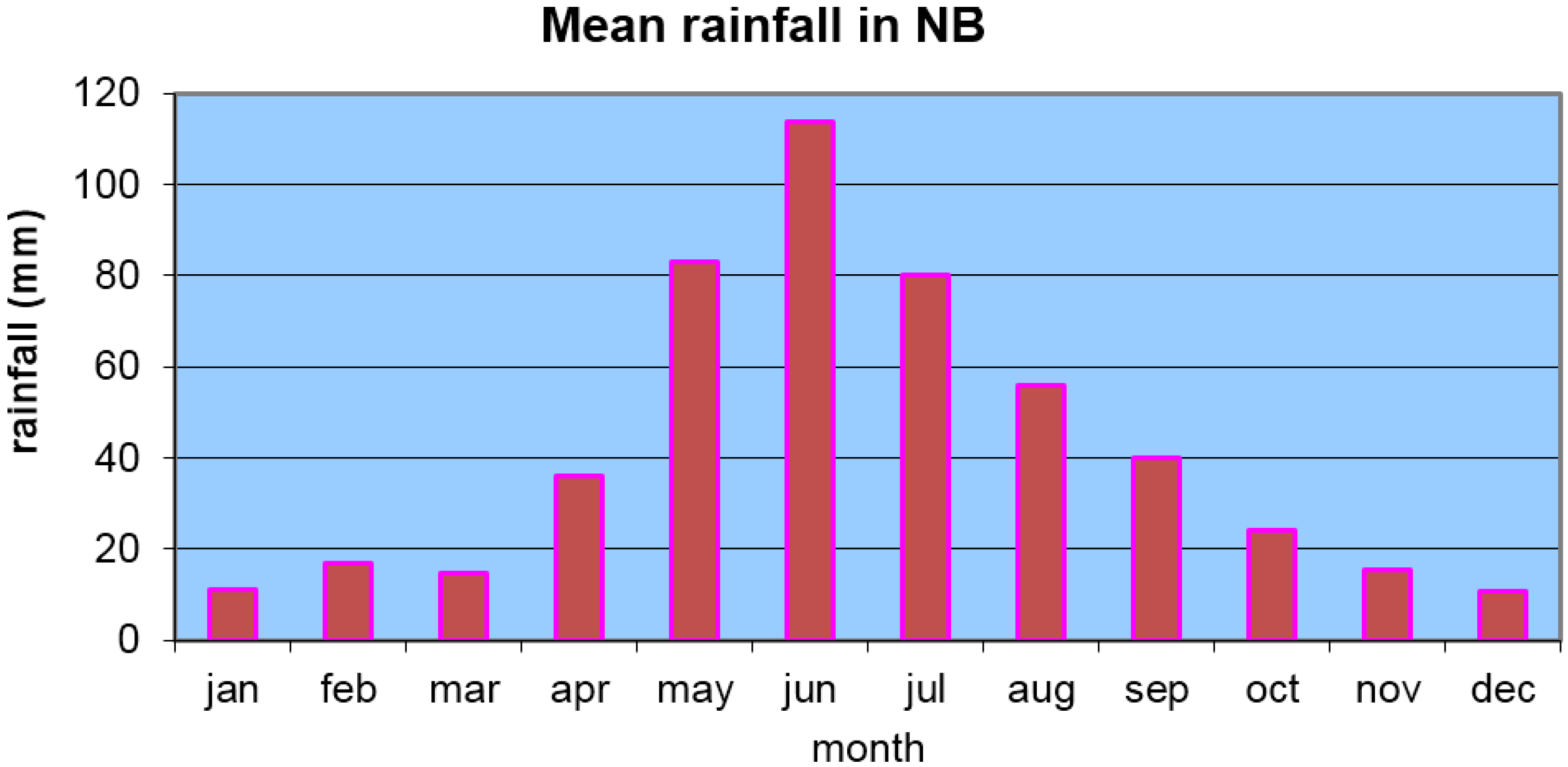
:1. Introduction
2. Data and Methodology


| Category | Definition | Frequency (%) | Years | |
|---|---|---|---|---|
| Extreme drought | SPI9 < −2 | 3.5 | 1998 | |
| Severe drought | −2 < SPI9 < −1.5 | 3.5 | 1996 | |
| DRY | Moderate drought | −1.5 < SPI9 < −1 | 10.7 | 1989, 1990, 2007 |
| CASES | Slight drought | −1 < SPI9 < −0.5 | 7.1 | 1985, 2003 |
| Normal | −0.5 < SPI9 < 0.5 | 39.3 | 1981, 1983, 1984, 1987, 1988, 1991, 1992, 1994, 1995, 1999, 2004 | |
| NORMAL | ||||
| CASES | ||||
| Slight excess | 0.5 < SPI9 < 1 | 21.4 | 1986, 1993, 1997, 2000, 2002, 2005 | |
| Moderate excess | 1 < SPI9 < 1.5 | 10.7 | 1980, 2001, 2006 | |
| WET | Severe excess | 1.5 < SPI9 < 2 | 3.5 | 1982 |
| CASES | Extreme excess | SPI9 > 2 | 0 | - |
3. Results and Discussion
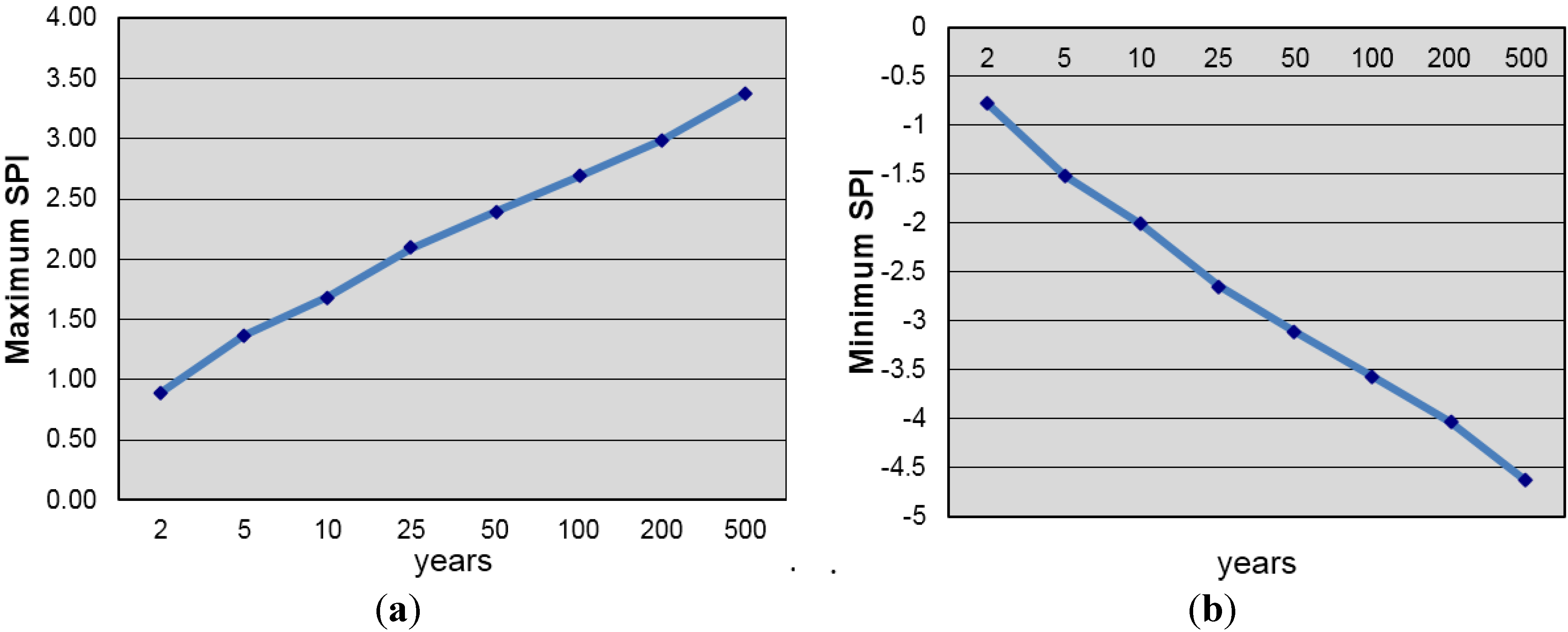
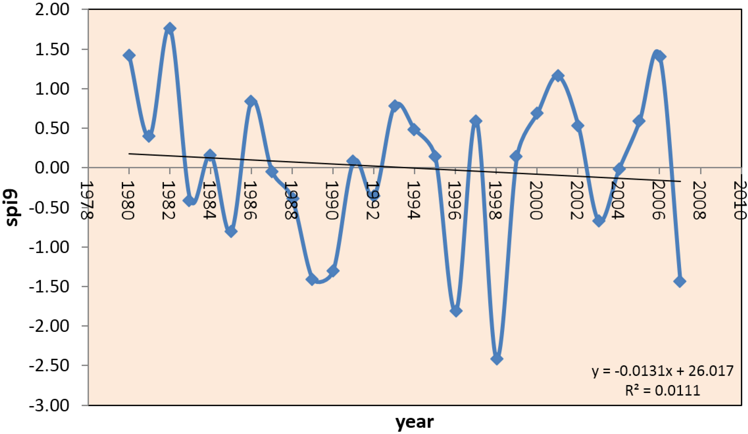
3.1. Low Frequency Standarized Precipitation Index Features in the Neuquén River Basin


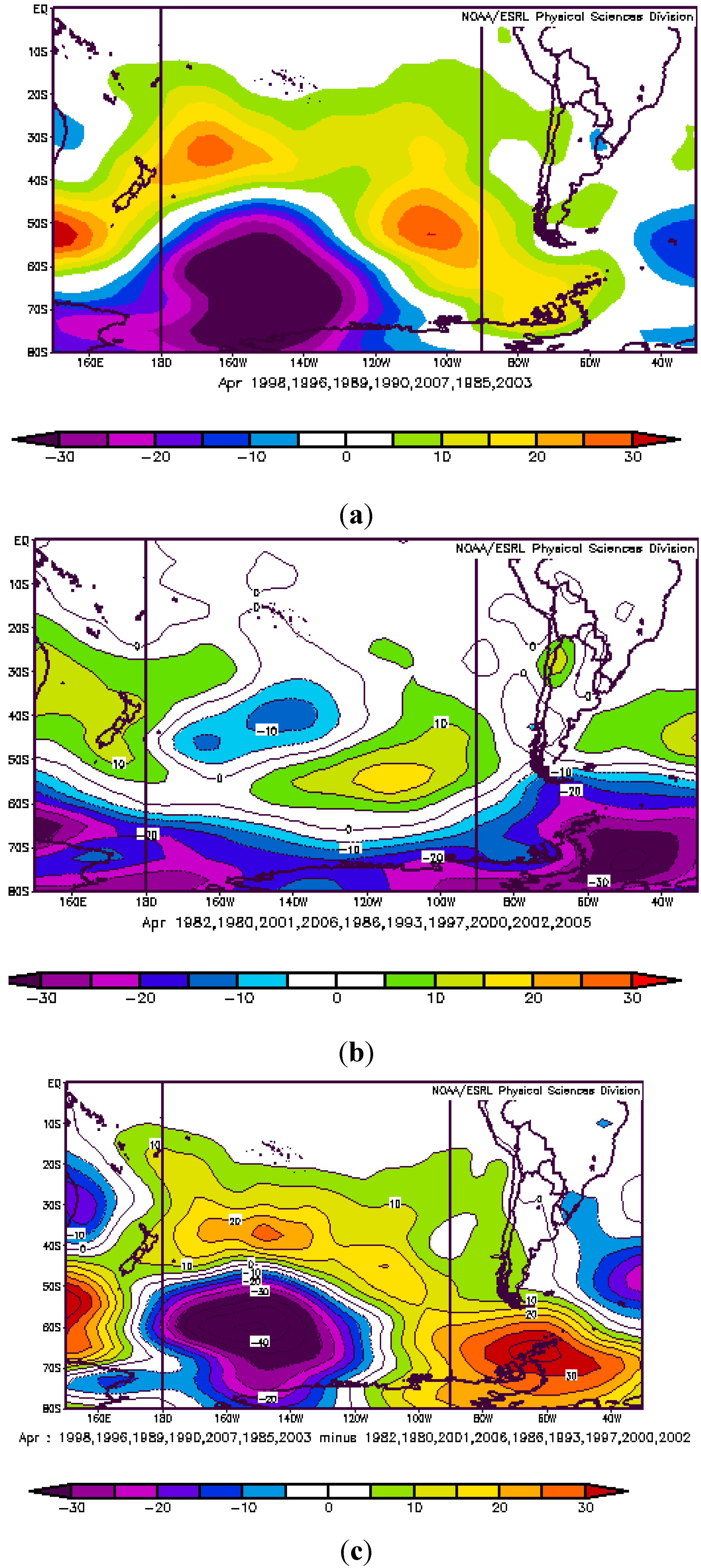
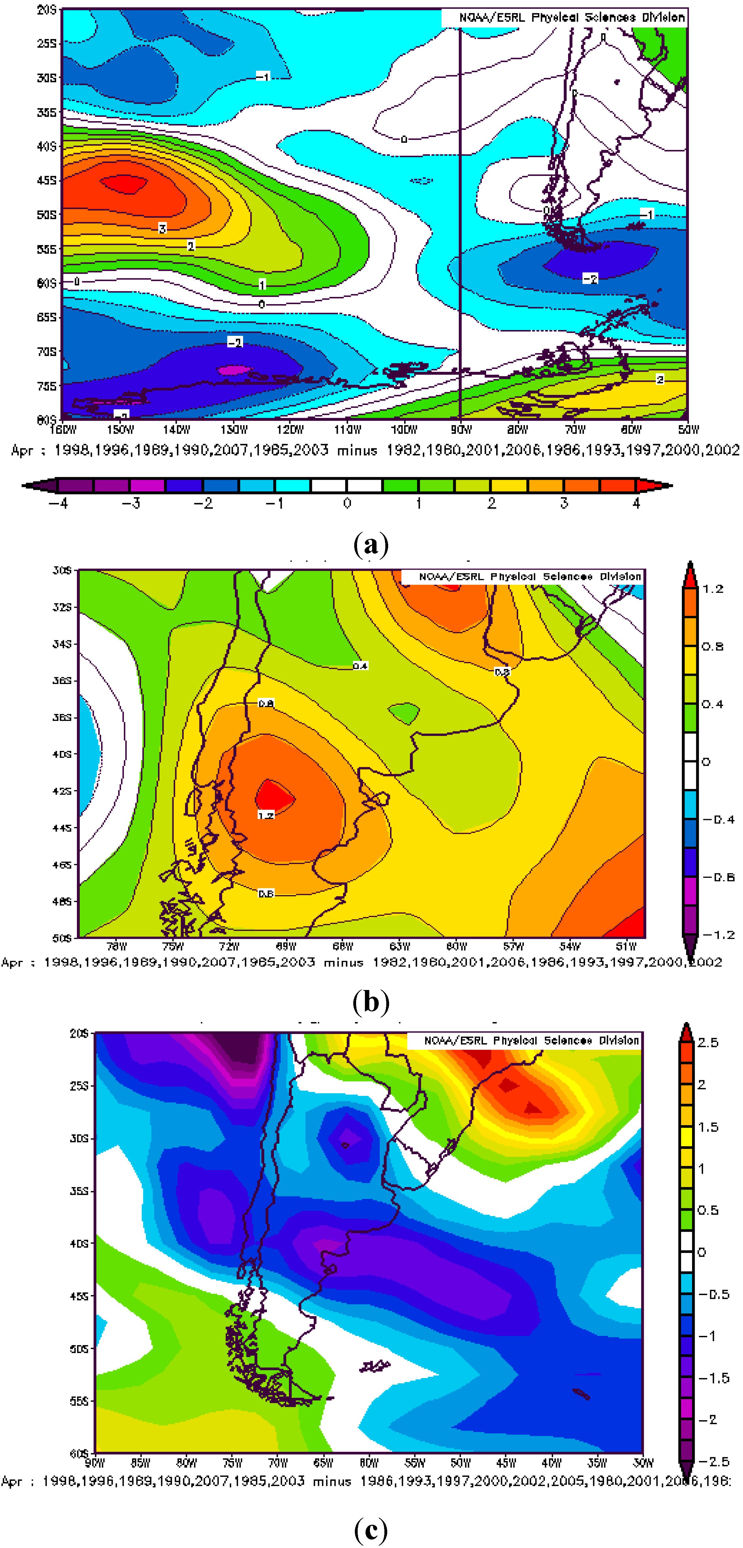
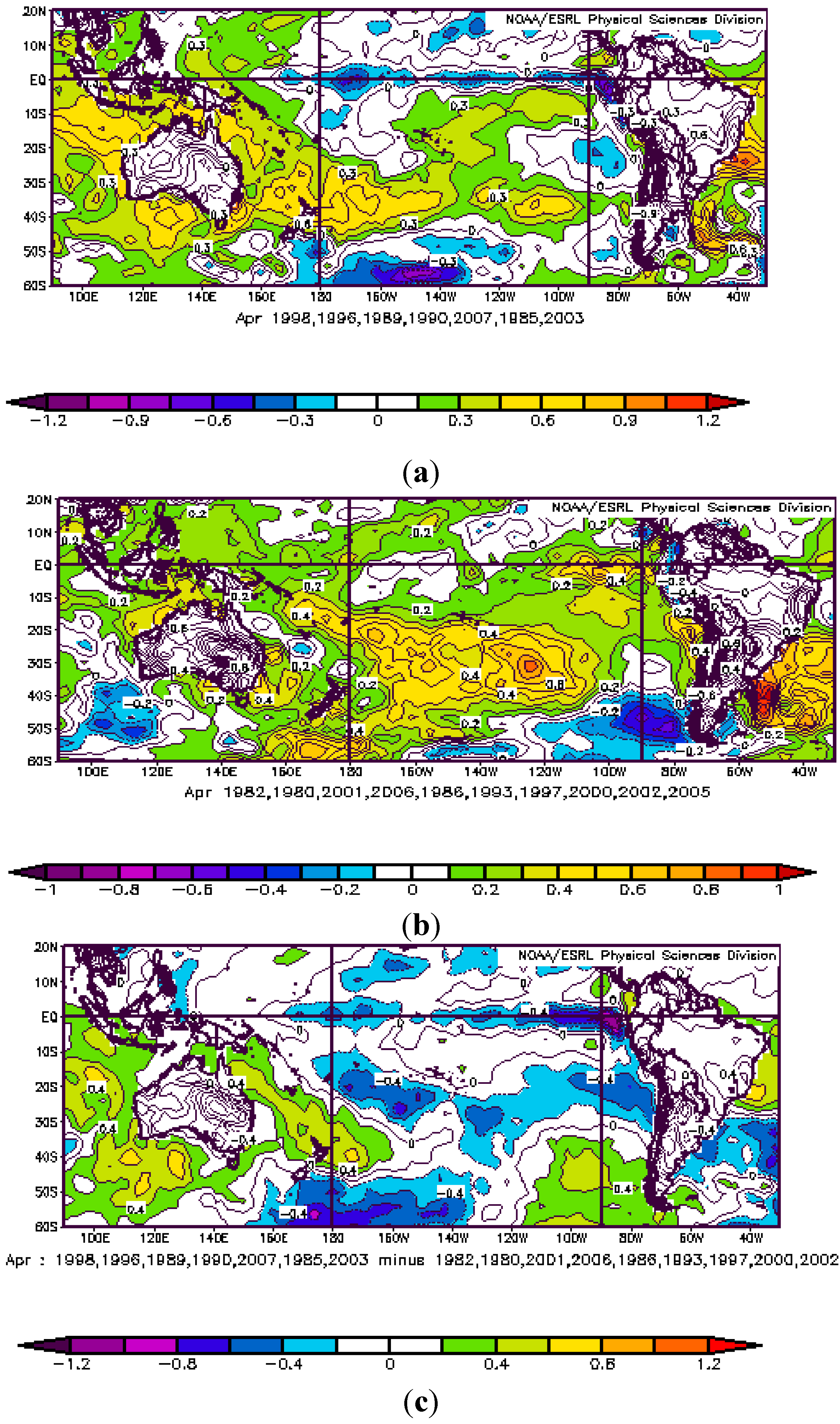
3.2. Atmospheric Circulation and Sea Surface Temperature Patterns Associated with Extreme Rainfall in the Neuquén River Basin
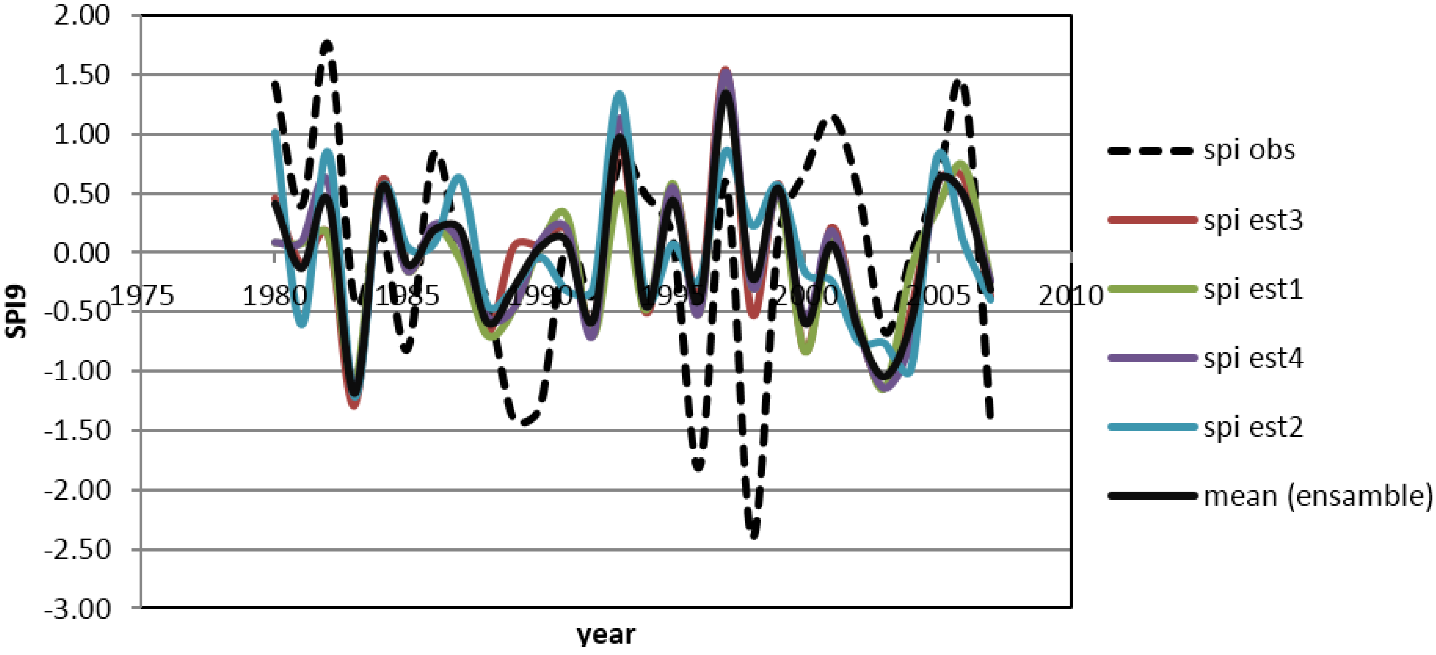
3.3. Statistical Models to Predict Extreme Rainfall in the Neuquén River Basin.


| Predictor | Variable | Area | Correlation |
|---|---|---|---|
| P1l | G1000 | (170°, 140°O; 55°, 70°S) | 0.39 |
| P1m | G500 | (170°, 140°O; 55°, 70°S) | 0.45 |
| P1h | G200 | (170°, 140°O; 55°, 70°S) | 0.35 |
| P2l | G1000 | (150°. 140°O; 35°, 40°S) | –0.49 |
| P2m | G500 | (150°, 140°O; 35°, 40°S) | –0.46 |
| P2h | G200 | (150°, 140°O; 35°, 40°S) | –0.4 |
| P3l | G1000 | (80°, 60°O; 60°, 75°S) | –0.33 |
| P3m | G500 | (80°, 60°O; 60°, 75°S) | –0.47 |
| P3h | G200 | (80°, 60°O; 60°, 75°S) | –0.43 |
| DNSl | G1000 | P1l–P2l | 0.55 |
| DNSm | G500 | P1m–P2m | 0.54 |
| DNSh | G200 | P1h–P2h | 0.43 |
| DEWl | G1000 | P1l–P3l | 0.47 |
| DEWm | G500 | P1m–P3m | 0.57 |
| DEWh | G200 | P1h–P3h | 0.51 |
| U1 | U | (155°, 140°O; 45°, 50°S) | –0.46 |
| V1 | V | (72°, 68°O; 42°, 44°S) | –0.13 |
| PW1 | PW | (65°, 55°O; 40°, 45°S) | 0.32 |
| SST1 | SST | (90°, 80°O; 5°N, 5°S) | –0.15 |
| SST2 | SST | (100°, 90°O; 40°, 50°S) | –0.37 |
| DEWm | G500 | P1m–P3m | 0.57 |
| Set | Predictors Entered in the Model | Explained Variance | Selected Predictors | Correlation between Observed and Predicted Spi9 |
|---|---|---|---|---|
| Set 1 | DNSm DEWm PW SST2 | 32 | DEWm | 0.42 |
| Set 2 | P1m P2m P3m SST2 PW | 43 | P2m P3m | 0.36 |
| Set 3 | DNSm P3m PW SST2 | 42 | DNSm P3m | 0.42 |
| Set 4 | DEWm P2m PW SST2 | 42 | DEWm P2m | 0.44 |
| Set | Regression Equation | F | p |
|---|---|---|---|
| Set1 | 0.007 DEWm + 0.001644 | 12.435 | 0.001 |
| Set 2 | −0.0132 P2m – 0.0101 P3m + 0.001644 | 9.75 | 0.0007 |
| Set 3 | 0.0057 DNS – 0.008 P3m + 0.001644 | 9.07 | 0.001 |
| Set4 | −0.009 P2m + 0.006 DEWm + 0.001644 | 9.33 | 0.0009 |
| POD | Below (SPI < 0) | Above (SPI > 0) | FAR | Below (SPI < 0) | Above (SPI > 0) |
|---|---|---|---|---|---|
| set1 | 0.79 | 0.93 | set1 | 0.08 | 0.19 |
| set2 | 0.6 | 0.77 | set2 | 0.25 | 0.38 |
| set3 | 0.69 | 0.8 | set3 | 0.25 | 0.25 |
| set4 | 0.77 | 0.87 | set4 | 0.17 | 0.19 |
| ensamble | 0.71 | 0.86 | ensamble | 0.17 | 0.25 |
4. Conclusions
Acknowledgments
References
- Gissila, T.; Black, E.; Grime, D.; Slingo, J.M. Seasonal forecasting of the Ethiopian summer rains. Int. J. Climatol. 2004, 24, 1345–1358. [Google Scholar] [CrossRef]
- Reason, C. Subtropical Indian Ocean SST dipole events and southern Africa rainfall. Geophys. Res. Lett. 2001, 28, 2225–2227. [Google Scholar] [CrossRef]
- Zheng, X.; Frederiksen, C. A study of predictable patterns for seasonal forecasting of New Zealand rainfall. J. Clim. 2006, 19, 3320–3333. [Google Scholar] [CrossRef]
- González, M.H.; Vera, C.S. On the interannual winter rainfall variability in southern Andes. Int. J. Climatol. 2010, 30, 643–657. [Google Scholar]
- González, M.H.; Skansi, M.M.; Losano, F. A statistical study of seasonal winter rainfall prediction in the Comahue region (Argentine). Atmosfera. 2010, 23, 277–294. [Google Scholar]
- González, M.H.; Herrera, N. Statistical prediction of winter rainfall in Patagonia (Argentina). In Horizons in Earth Science Research, 1st ed.; Veress, B., Szigethy, J., Eds.; NOVA Science Publishers: Hauppauge, NY, USA, 2014; Volume 11, pp. 221–238. [Google Scholar]
- Scarpati, O.; Kruse, E.; Gonzalez, M.H.; Ismael, A.; Vich, J.; Capriolo, A.; Caffera, R. Updating the Hydrological Knowledge: A case of Study. In Handbook of Engineering Hydrology, Environmental Hydrology and River Management, 1st ed.; Eslamian, S., Ed.; Taylor & Francis Group LLC: Boca Raton, FL, USA, 2014; Volume 3, pp. 443–457. [Google Scholar]
- González, M.H. Some indicators of interannual rainfall variability in Patagonia (Argentine). In Clim. Variability––Regional and Thematic Patterns, 1st ed.; Tarhule, A., Ed.; INTECH: London, UK, 2013; pp. 133–161. [Google Scholar]
- González, M.H.; Dominguez, D. Statistical prediction of wet and dry periods in the Comahue Region (Argentina). Atmos. Clim. Sci. 2012, 2, 2160–2414. [Google Scholar]
- Mckee, T.; Doesken, N.; Kleist, J. The relationship of drought frequency and duration to times scales. In Proceedings of the Eighth Conference of Applied Climatology, Anaheim, CA, USA, 17–22 January 1993.
- McKee, T.; Doesken, N.; Kleist, J. Drought monitoring with multiple time scales. In Proceedings of the Ninth Conference on Applied Climatology, Dallas, TX, USA, 15–20 January 1995.
- Garbarini, E.M.; Gonzalez, M.H. Variabilidad de la Precipitación en Argentina: Factores de Influencia. In the Proceedings of 2do Congreso Internacional de Hidrología de Llanuras, Santa Fe, Argentina, 23–26 September 2014.
- Hayes, M.; Svoboda, M.; Wilhite, D.; Vanyarkho, O. Monitoring the 1996 drought using the standardized precipitation index. Bull. Am. Meteorol. Soc. 1999, 80, 429–438. [Google Scholar] [CrossRef]
- Heim, R. A review of Twentieth Century drought indices used in the United States. Bull. Am. Meteorol. Soc. 2002, 83, 1149–1165. [Google Scholar]
- Mitchell, J.M.; Dzerdzeevskii, B.; Flohn, H.; Hofmeyr, W.L.; Lamb, H.H.; Rao, K.N.; Walléen, C.C. Climatic Change; Technicall Note No. 79; World Meteorological Organization (WMO): Geneva, Switzerland, 1966. [Google Scholar]
- Blackman, R.B.; Tukey, J.W. The Measurement of Power Spectral from the Point of View of Communication Engineering; Dover: New York, NY, USA, 1958. [Google Scholar]
- Kalnay, E.; Kanamitsu, M.; Kistler, R.; Collins, W.; Deaven, D.; Gandin, L.; Iredell, M.; Saha, S.; White, G.; Woollen, J.; et al. The NCEP/NCAR reanalysis 40 years-project. Bull. Am. Meteor. Soc. 1996, 77, 437–471. [Google Scholar] [CrossRef]
- Wilks, D. Statistical Methods in the Atmospheric Sciences: An Introduction, 2nd ed.; Elsevier: San Diego, CA, USA, 1995. [Google Scholar]
- Darlington, R.B. Regression and Linear Models; McGraw-Hill: New York, NY, USA, 1990. [Google Scholar]
- Kidson, J. Principal modes of southern hemisphere low frequency variability obtained from NCEP-NCAR reanalyses. J. Clim. 1999, 1, 1177–1198. [Google Scholar] [CrossRef]
- Mo, K.C. Relationships between low frequency variability in the southern Hemisphere and sea surface temperature anomalies. J. Clim. 2000, 13, 3599–3610. [Google Scholar] [CrossRef]
- Nogues Paegle, J.; Mo, K.C. Linkages between summer rainfall variability over South America and sea surface temperature anomalies. J. Clim. 2002, 15, 1389–1407. [Google Scholar] [CrossRef]
© 2015 by the author; licensee MDPI, Basel, Switzerland. This article is an open access article distributed under the terms and conditions of the Creative Commons Attribution license (http://creativecommons.org/licenses/by/4.0/).
Share and Cite
González, M.H. Statistical Seasonal Rainfall Forecast in the Neuquén River Basin (Comahue Region, Argentina). Climate 2015, 3, 349-364. https://doi.org/10.3390/cli3020349
González MH. Statistical Seasonal Rainfall Forecast in the Neuquén River Basin (Comahue Region, Argentina). Climate. 2015; 3(2):349-364. https://doi.org/10.3390/cli3020349
Chicago/Turabian StyleGonzález, Marcela Hebe. 2015. "Statistical Seasonal Rainfall Forecast in the Neuquén River Basin (Comahue Region, Argentina)" Climate 3, no. 2: 349-364. https://doi.org/10.3390/cli3020349