Structural Breaks, Inflation and Interest Rates: Evidence from the G7 Countries

Abstract

This study reconsiders the common unit root/co-integration approach to test for the Fisher effect for the economies of the G7 countries. We first show that nominal interest and inflation rates are better represented as I(0) variables. Later, we use the Bai–Perron procedure to show the existence of structural changes in the Fisher equation. After considering these breaks, we find very limited evidence of a total Fisher effect as the transmission coefficient of the expected inflation rates to nominal interest rates is very different than one.

1. Introduction

One of the most important results from classical economic theory is that the movements of nominal variables have no impact on real economic variables. This result, which can be verified by testing the long-run neutrality proposition, implies that a permanent movement in the inflation rate has no effect on the equilibrium real interest rate. The traditional way to represent this phenomenon is to decompose nominal interest rates into two separate components that reflect expected inflation and the “real” interest rate. Following Fisher’s (1930) study [1], which is very influential, this relationship can be stated through the well-known Fisher equation:

$$R_t={\pi }_t^e+r_t$$

(1)

where R represents the nominal interest rate, ${\pi }^e$ is the expected rate of inflation and r is the (ex-ante) real interest rate. In simple economic models, this last variable is determined by deep structural parameters, such as investor preferences or the marginal efficiency of capital, and is often assumed to be constant over long horizons. According to (1), moneylenders need a nominal interest rate that compensates them for the purchasing power lost over the duration of the loan, which is proxied by the expected inflation. Thus, if there is no money illusion, then a change in the expected inflation rate should be fully transmitted to the nominal interest rate to maintain a constant real interest rate.

Equation (1) provides useful information, both for theoretical research and for those making economic policy decisions. For example, if the Fisher effect holds, then the expected inflation is a good predictor of the nominal interest rate. Further, there is evidence of the superneutrality of money hypothesis. Consequently, it comes as no surprise that a significant body of literature analyzes the relationship between nominal interest rates and inflation or, more exactly, whether the so-called Fisher effect holds. The most common approach starts by estimating the following equation:

$$R_t=\alpha +\beta {\pi }_{t+1}+e_t$$

(2)

which implicitly assumes the presence of perfect rational expectations (${\pi }_{t+1}={\pi }_t^e$) and that α reflects the (ex-ante) real interest rate. It is clear that, whenever the value of the parameter β, often referred to as the Fisher coefficient, is equal to one, this equation is equal to (1), and therefore, we should conclude that the Fisher effect holds. At first sight, the analysis of this effect appears to be quite straightforward, in the sense that it only requires an estimation of (2) and a subsequent test of the null hypothesis H_o: $\beta =1$. However, the literature confirms that there are several points that should be considered to accurately estimate this parameter and to test this hypothesis. Our study proposes a different statistical methodology to test the relationship between inflation and the nominal interest rate, adding to the controversy over which technique is the most suitable for testing the Fisher effect. 1 Here, we consider the appropriate treatment of the time series properties of the variables, as well as the possible presence of changes in the values of the parameters α and β. In this study, we consider the importance of these two points.

With respect to the first, there seems to be an almost unanimous opinion in the literature about the existence of unit roots in both the nominal interest rate and the inflation rate. Therefore,”standard” econometric models are no longer valid; rather, the co-integration approach should be employed. There are several examples of the use of this unit root/co-integration approach, beginning with the seminal studies of Rose (1988) [4] and Mishkin (1992) [5], whose methodology was subsequently applied in the more recent studies of Crowder and Wohar (1999) [6], Koustas and Serletis (1999) [7], Rapach (2002) [8], Laatsch and Klein (2003) [9] and Rapach and Weber (2005) [10], amongst many others. Some recent studies opted to use the panel data unit root/co-integration approach, as is the case of Westerlund (2008) [11] and Ozcan and Ari (2015) [12].

Nevertheless, some authors, such as Cox et al. (1985) [13], Malliaropoulos (2000) [14], Lanne (2001) [15], Olekalns (2001) [16], Gil-Alaña (2002) [17] and Atkins and Coe (2002) [18], questioned the presence of a unit root in the evolution of both the nominal interest rate and the inflation rate. Similarly, some other authors suggest the possibility that these variables may follow a long-memory process. We can cite the papers of Baum et al. (1999) [19], Phillips and Perron (1998) [20], Tsay (2000) [21], Sun and Phillips (2004) [22], Gil-Alaña (2004) [23] and Gil-Alaña and Moreno (2012) [24], in the case of the nominal interest rate, and Hassler and Wolters (1995) [25] and Bos et al. (1999) [26] with respect to the inflation rate. In light of this, the use of the unit root/co-integration approach is now open to debate.

In addition to the doubts raised by the authors above, we tentatively offer a new source of criticism in this study based on the potential non-constancy of the parameters included in the Fisher equation in the spirit of Lucas’s critique (Lucas (1976) [27]). Our argument is based on the fact that most of the studies analyzing the Fisher effect use sample sizes covering the period from the 1970s to the present day. However, none of these appear to account for the different monetary policies in effect during this very lengthy period of time, making the constant parameter hypothesis doubtful. Instead, we argue that it is more appropriate to consider the hypothesis that some structural breaks affect the Fisher relationship. They may arise, if we consider that the presence of which can be understood if we consider, for example, that the real interest rate is the consequence of the interaction between savings and investment, and it may change when savings owners modify their behavior.

In this regard, and as Chadha and Dimsdale (1999) [28] point out, demographic change, technological progress, fiscal incentives, changes in the taxation of profits, the size of the public debt, investors’ perception of risk and the degree of regulation or deregulation of capital markets could alter the constant and inflation parameters. Another source of possible variation in the parameters of (2) comes from the fact that the influence of inflation on the nominal interest rate can also vary. More robust inflation targeting and a more active monetary policy, as indicated by Söderlind (2001) [29] and Olekalns (2001) [16], or constraints on capital markets could be important determinants of the final value of these parameters.

Against this background, this study aims to analyze the Fisher effect for the G7 group of countries by explicitly accounting for the both variables and, more importantly, that the presence of structural breaks can affect the parameters of the Fisher equation. In order to illustrate this starting hypothesis, we begin by testing the time series properties of nominal interest and inflation rates. If we can find evidence that leads us to better characterize these variables as being I(0), then we should not use the co-integration approach because applying, similar arguments as Malliaropoulos (2000) [14] does, this may lead to spurious evidence of the Fisher effect. Furthermore, and in order to reflect the possible non-constancy of the Fisher equation, we allow for the presence of some breaks in the relationship between the nominal interest rate and the inflation rate. In a stationary scenario, we can apply Bai and Perron’s (1998, 2003) [30,31] proposed procedure to test for the stability of the Fisher effect equation. This method also has the advantage of providing consistent estimations of both the number of breaks and the periods when these occur. Finally, we can use the results obtained by applying these techniques to estimate the Fisher relationship when we incorporate the structural breaks and the dynamic effects.

The rest of the paper is organized as follows. In Section 2, we describe the tests we employ to test for the time series properties of the variables. When these are applied to the nominal interest and inflation rates of the economies of the G7 countries, we find that they allow us to reject the unit root null hypothesis, a result that suggests that it is more advisable to analyze the Fisher effect in a stationary framework, rather than in a non-stationary one. In light of this result, in Section 3, we first propose the use of the Bai–Perron procedure to determine the presence of structural breaks in the Fisher equation. We then apply this procedure to analyze the Fisher effect for the economies of the G7 countries. Section 4 closes the paper with a review of the most important conclusions.

2. Fisher Effect with Non-Integrated Variables

Following Nelson and Plosser’s (1982) seminal study [32], most empirical analyses based on the use of variables measured as time series begin by studying the time properties of the variables. If these are better characterized as being integrated, then researchers use co-integration techniques. If, by contrast, they are stationary, then we can use standard econometric techniques. The study of the Fisher effect is a scenario in which we can clearly appreciate the application of this strategy and, since Mishkin’s (1992) [5] classic study, most of the literature devoted to this issue has followed such an approach.

However, some studies appear to have raised some questions about the appropriateness of the unit root model when seeking to accurately describe the evolution of both inflation rates and nominal interest rates. Malliaropoulos (2000) [14] and Baum et al. (1999) [19] showed that USA nominal interest and inflation rates can be better represented using broken trend stationary models. This finding is very important in the sense that, at least for the USA data, it casts doubts on the adequacy of the co-integration approach to test for the Fisher effect. A common method under this approach is to test whether the real interest rate is integrated. If we can conclude that the real interest rate is not integrated, this will be interpreted as evidence of the Fisher effect. However, this method is only valid when the nominal interest rate and the expected inflation rate are integrated. To better appreciate this, let us consider an expected inflation (π) and a nominal interest rate (R) represented as I(0) variables. Any combination of these variables, say R − β π, will also be an I(0) variable. However, this does not imply that the Fisher effect holds, because it only does so when the parameter β is one. Thus, in the presence of I(0) variables, admitting that the real interest rate is not integrated, does not necessarily imply that the Fisher effect holds.

This finding requires a careful analysis of the time properties of the nominal interest rates and inflation rates, which is precisely the aim of the next subsection.

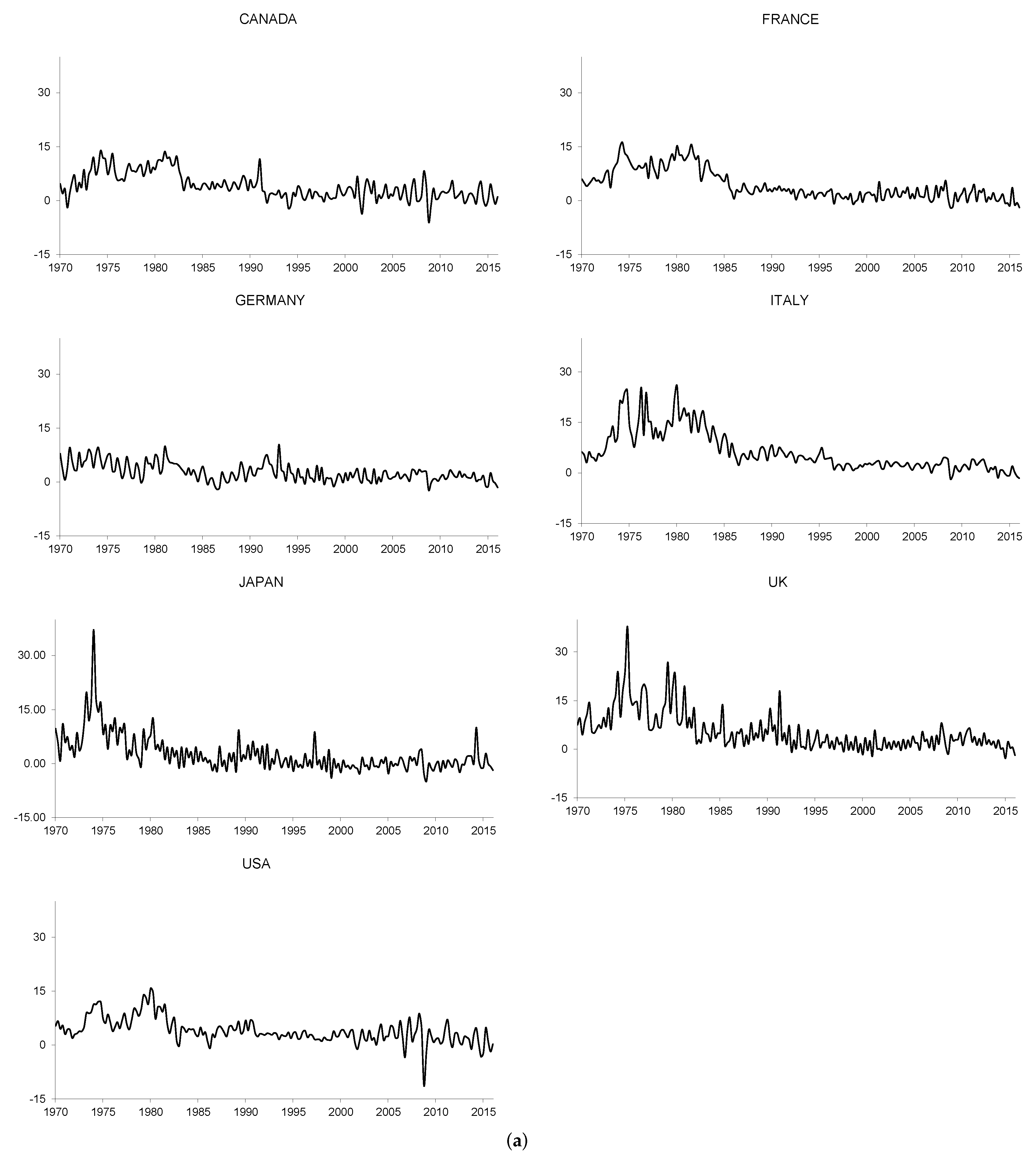
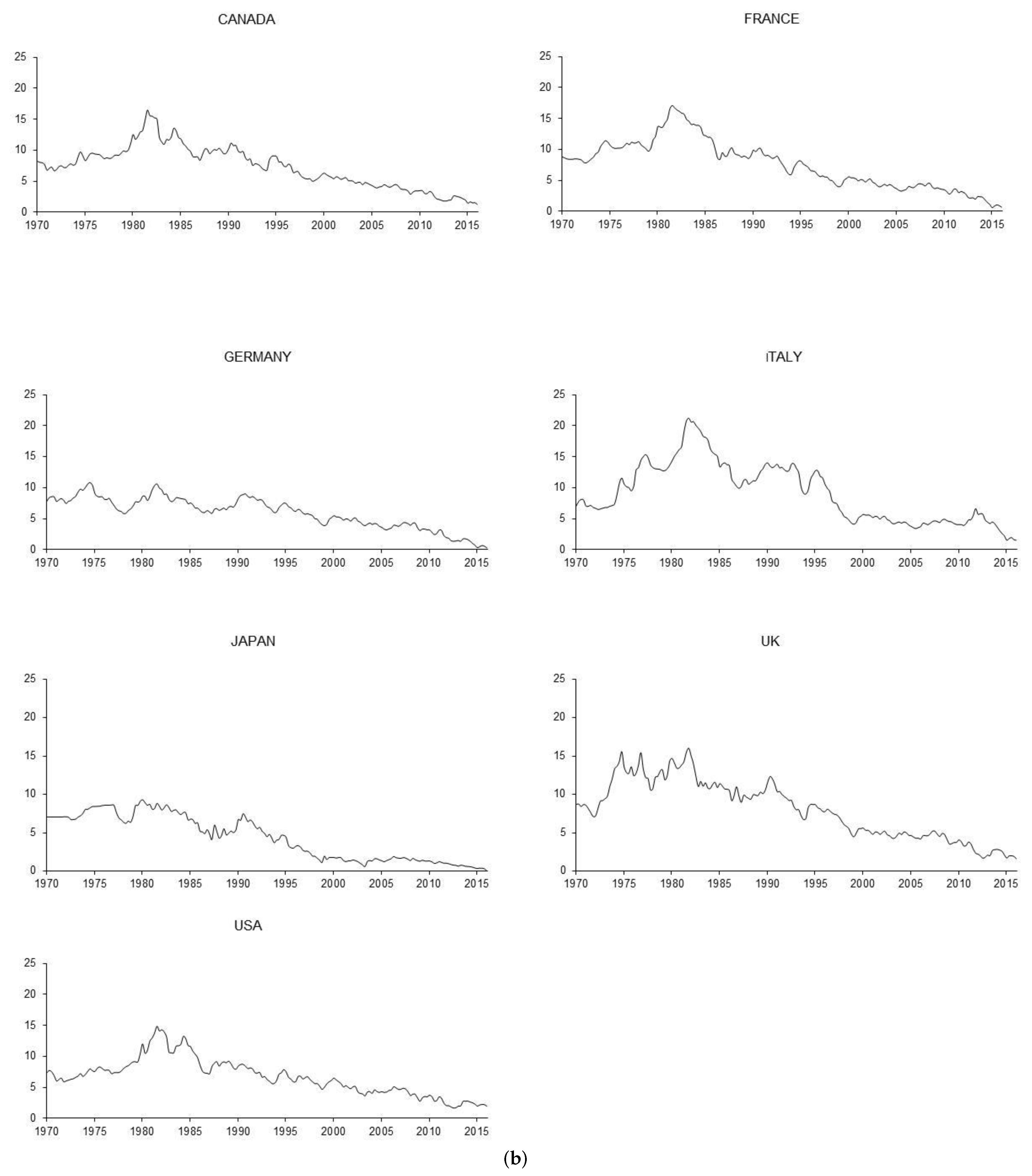
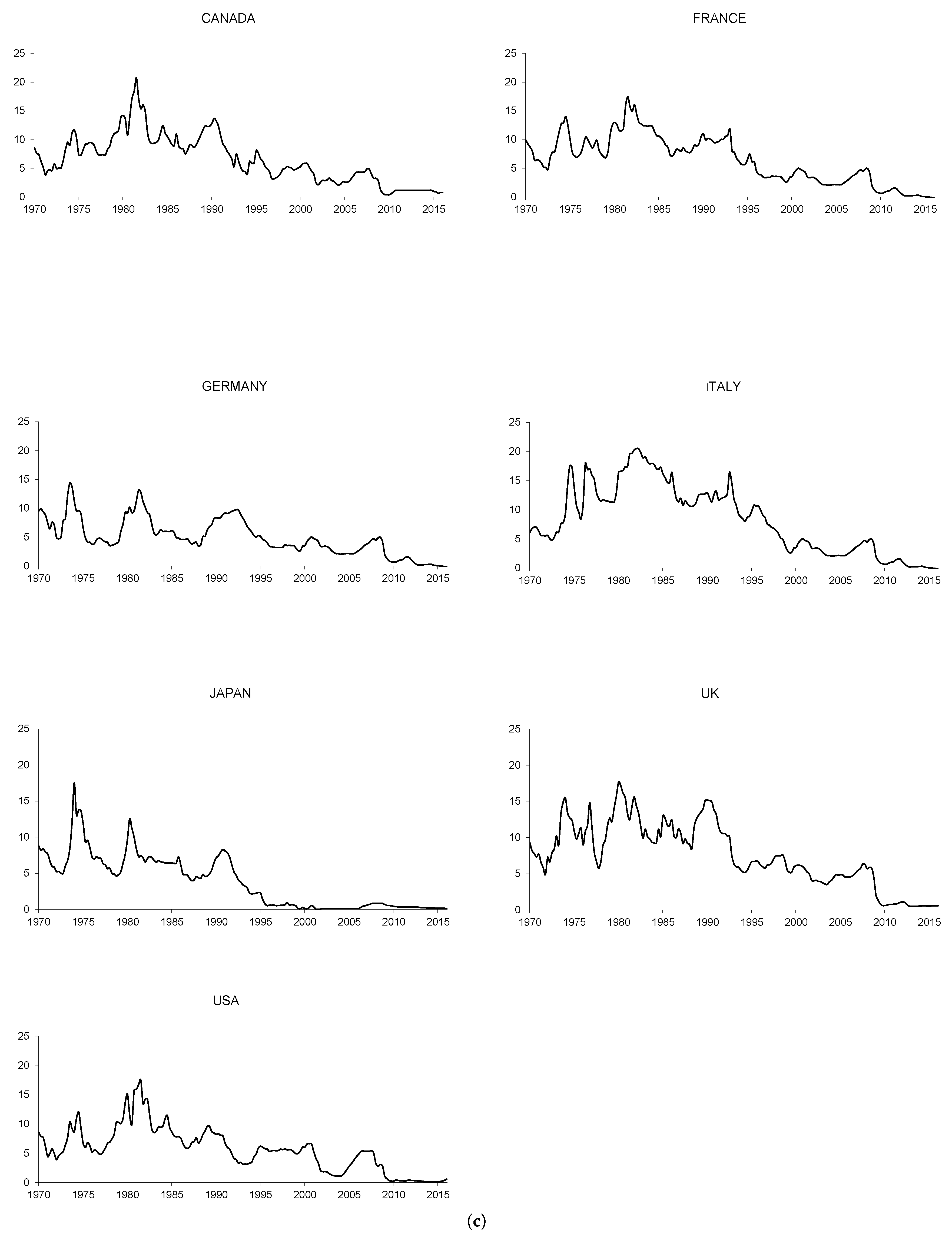
2.1. Analysis of the Time Properties of the Nominal Interest Rates and Inflation Rates

We have already made the point that an analysis of the time properties of the nominal interest rates and inflation rates should be carried out carefully, and should certainly not be regarded as just a prior step in using co-integration techniques. There is a great range of statistics devoted to this issue. For example, most of the studies related to this area base their analysis on augmented Dickey–Fuller (ADF) tests (Dickey and Fuller (1979) [33]; Said and Dickey (1984) [34]), the methods presented in Phillips and Perron (1988) [20] or subsequent modifications of these types of statistics proposed by Ng and Perron (2001) [35], which compare the performance of a wide range of unit root statistics. For example, these authors consider the ADF^GLS, which is based on the very popular ADF test. Following Elliot et al. (1996) [36], this can be obtained by estimating the following model:

$$y_t={\delta }_t+\rho y_{t-1}+{\displaystyle \sum _{i=1}^{\ell }}{\varphi }_i\Delta y_{t-i}+{\epsilon }_t$$

(3)

where $\delta {}_t$ reflects the deterministic elements, 2 and subsequently calculating the pseudo t-ratio to test whether the parameter ρ is one. The differences between this and the simple ADF test lie in the fact that ADF^GLS is based on the use of GLS (Generalized Least Squares) estimation methods instead of OLS (Ordinary Least Squares) estimators and on determining the value of the lag truncation parameter (ℓ) by using an information criterion, called MIC (Modified Information Criteria), also proposed in Ng and Perron (2001) [35]. This type of statistics is not useful to reject the presence of a unit root in nominal interest rates and inflation. This is why some authors have recently employed different statistics to analyze the time series properties of the variables to take advantage of the cross-sectional information of a database. Thus, it seems suitable to use a panel data approach to test for the presence of a unit root in the variables in the Fisher equation. In order to select the most appropriate type of panel data unit root test, we should first know the characteristics of the database, because of the possible presence of a cross-sectional correlation between the variables.

It is common to begin by testing for the null hypothesis of cross-sectional independence using Pesaran’s (2004) CD (Cross Dependence) statistic [37], which has the following definition:

$$CD=\sqrt{\frac{2T}{N}{\displaystyle \sum _{j=1}^N}{\widehat{\rho }}_j^2}\sim N(0,1)$$

(4)

where T is the sample size, N the cross-sectional dimension and $\widehat{\rho }$ is the pair-wise Pearson’s correlation coefficients ${\widehat{\rho }}_j$, $j=1,\dots ,n$, $n=N(N-1)/2$ of the residuals obtained from augmented Dickey–Fuller type regression equations. If we cannot reject this null hypothesis, then we should use the CIPS statistics because they correct the distortion caused by the cross-sectional correlation. Following Pesaran (2007) [38], the CIPS (cross-sectionally augmented panel unit root test) statistic is defined as follows:

$$CIPS=N^{-1}{\displaystyle \sum _{i=1}^N}{\overline{t}}_i$$

(5)

with ${\overline{t}}_i$ being the OLS t-ratio to test the H_o:${\alpha }_i=0$ in the following cross-sectional ADF regressions:

$$\Delta y_{it}={\delta }_{it}+{\alpha }_i{y}_{it-1}+{\gamma }_i{\overline{y}}_{t-1}+{\displaystyle \sum _{j=1}^p}{\varphi }_{ij}\Delta y_{i,t-j}+{\displaystyle \sum _{j=0}^p}{\phi }_{ij}\Delta {\overline{y}}_{t-1}+{\epsilon }_{it}$$

(6)

where ${\overline{y}}_{t-1}$ denotes the cross-sectional mean of $y_{it}$. Tables II(a)–(c) in Pesaran (2007) [38] provide the critical values for the CIPS tests, in addition to a proposed truncated version of this statistic, commonly referred to as CIPS*, which will be used in the following section.

2.2. Empirical Evidence from the G7 Countries

As we mentioned earlier, the methodology to employ to analyze the Fisher effect depends on the time properties of the variables that are necessary to study it, namely the nominal interest rates and inflation rates. Thus, we should be careful when determining the integration order of these variables. To that end, we apply the statistics presented in the previous section to the nominal interest rates and inflation rates of the G7 countries. We take two different measures of the nominal interest rates. First, we select a short-run variable, measured through the three-month treasury bill rate (or equivalent) for each sample country. Second, we take the 10-year government bond (or equivalent) for each sample country as a measure of the long-run behavior of nominal interest rates. We obtain the annualized inflation rates from the Consumer Price Index (CPI). We obtain all data from the OECD Main Economic Indicators. Finally, the quarterly data, where possible, cover the sample period 1970:Q1–2015:Q4. 3 Figure 1, Figure 2 and Figure 3 illustrate these variables, whilst

Table 1. Testing for cross-sectional dependence.

	Long-Run Nominal Interest	Short-Run Nominal Interest	Inflation
p = 0	29.25 *	19.13 *	20.06 *
p = 1	26.33 *	15.39 *	20.32 *
p = 2	25.85 *	15.52 *	19.27 *
p = 3	25.16 *	15.32 *	19.83 *
p = 4	24.76 *	15.28 *	18.78 *

This table reports the values of the CD (Cross Dependence) statistic proposed in Pesaran (2004) [37] to test the non-cross-sectional dependence null hypothesis. The values were obtained by estimating a Dickey–Fuller-type equation without trend, with fixed effects and for different lag values (p = 1,..,4). *: rejection of the null hypothesis even for a demanding 1%.

and

Table 2. CIPS* panel data unit root tests.

	Long-Run Nominal Interest	Short-Run Nominal Interest	Inflation
p = 0	−2.89 **	−6.73**	−12.94 **
p = 1	−3.08 **	−7.19**	−12.46 **
p = 2	−2.27 *	−6.14**	−10.79 **
p = 3	−2.38 **	−5.67**	−7.52 **
p = 4	−2.36 **	−5.87**	−7.50 **

This table reports the values of the CIPS* (cross-sectionally augmented panel unit root test, truncated version) statistic proposed in Pesaran (2007) [38] to test the unit root null hypothesis. The values were obtained by estimating (6), where the specification includes only an intercept. ** and *: rejection of the null hypothesis at the 5% and the 1% significance level, respectively.

report the results of applying the previously-mentioned statistics to our database.

Table 1 reflects the results of the CD statistic to test the null hypothesis of no cross-sectional dependence. We can easily reject this null hypothesis, and consequently, we should employ panel data unit root tests that account for its presence. The CIPS* statistic, whose results are presented in Table 2, takes into account the cross-sectional dependence. As we can see, there is only very robust evidence against the unit root null hypothesis. However, some countries may exhibit the presence of the unit root in any of the analyzed variables. 4 In order to explore this possibility, we have considered several subgroups of countries. We have taken all of the possible combinations of five and six countries, and the values of the CIPS* statistic always allows the rejection of the null hypothesis, the average p-value being lower than 0.01 Thus, this lack of evidence against the null hypothesis matches the results of Constantini and Lupi (2007) [40] and Lee and Chang (2007, 2008) [41,42], who reject the presence of a unit root in the inflation rate for different sample sizes of OECD countries using the LM (Lagrange Multiplier) tests proposed in Lee and Strazicich (2003, 2013) [43,44], which consider the presence of broken trends in the evolution of these variables. These statistics can also provide evidence against the unit root null hypothesis for the nominal interest rates, as is reflected in Gadea et al. (2009) [45]. Thus, the global consideration of all of this evidence leads us to an analysis of the Fisher effect using I(0) variables instead of the much more common approach of using I(1) variables.

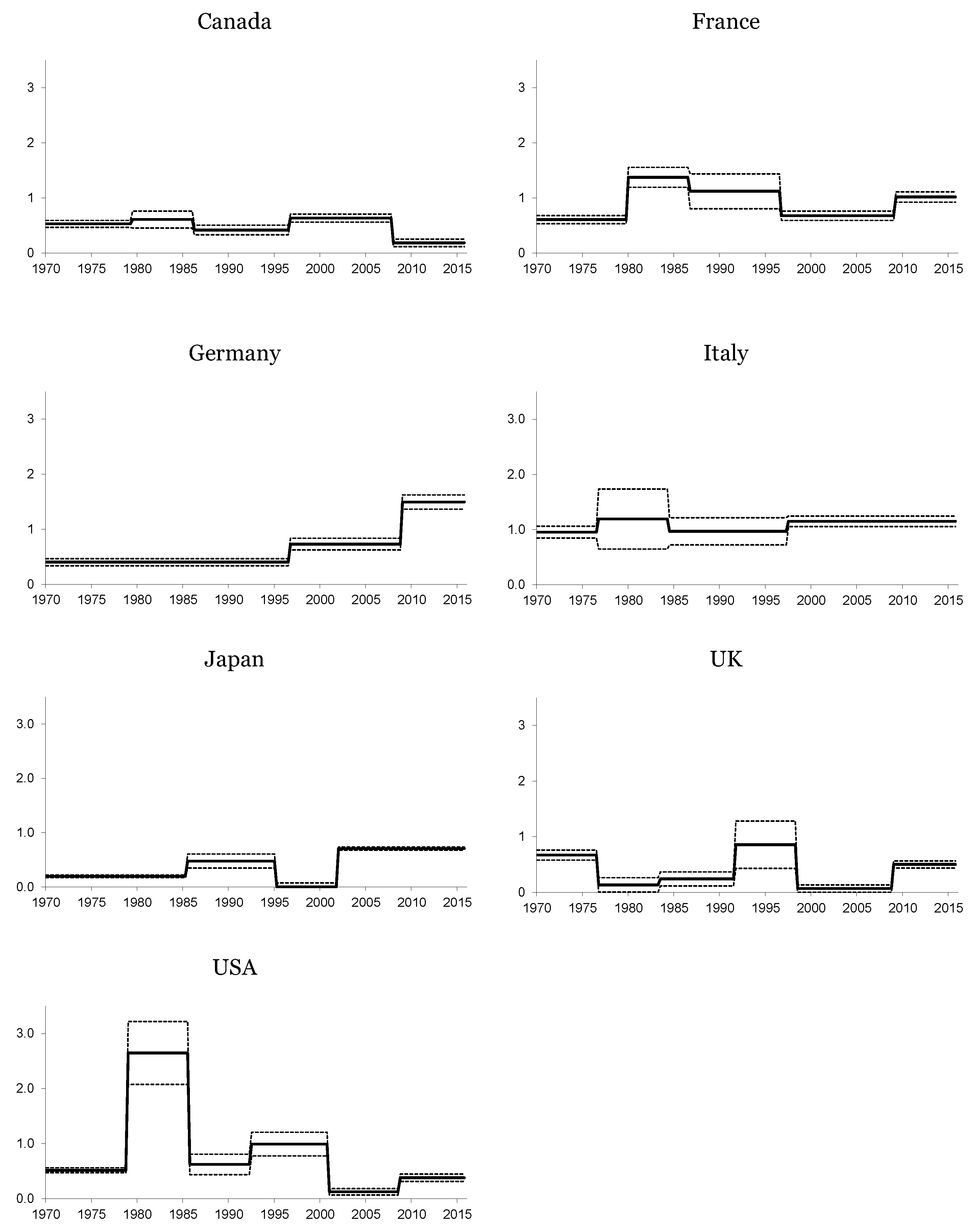
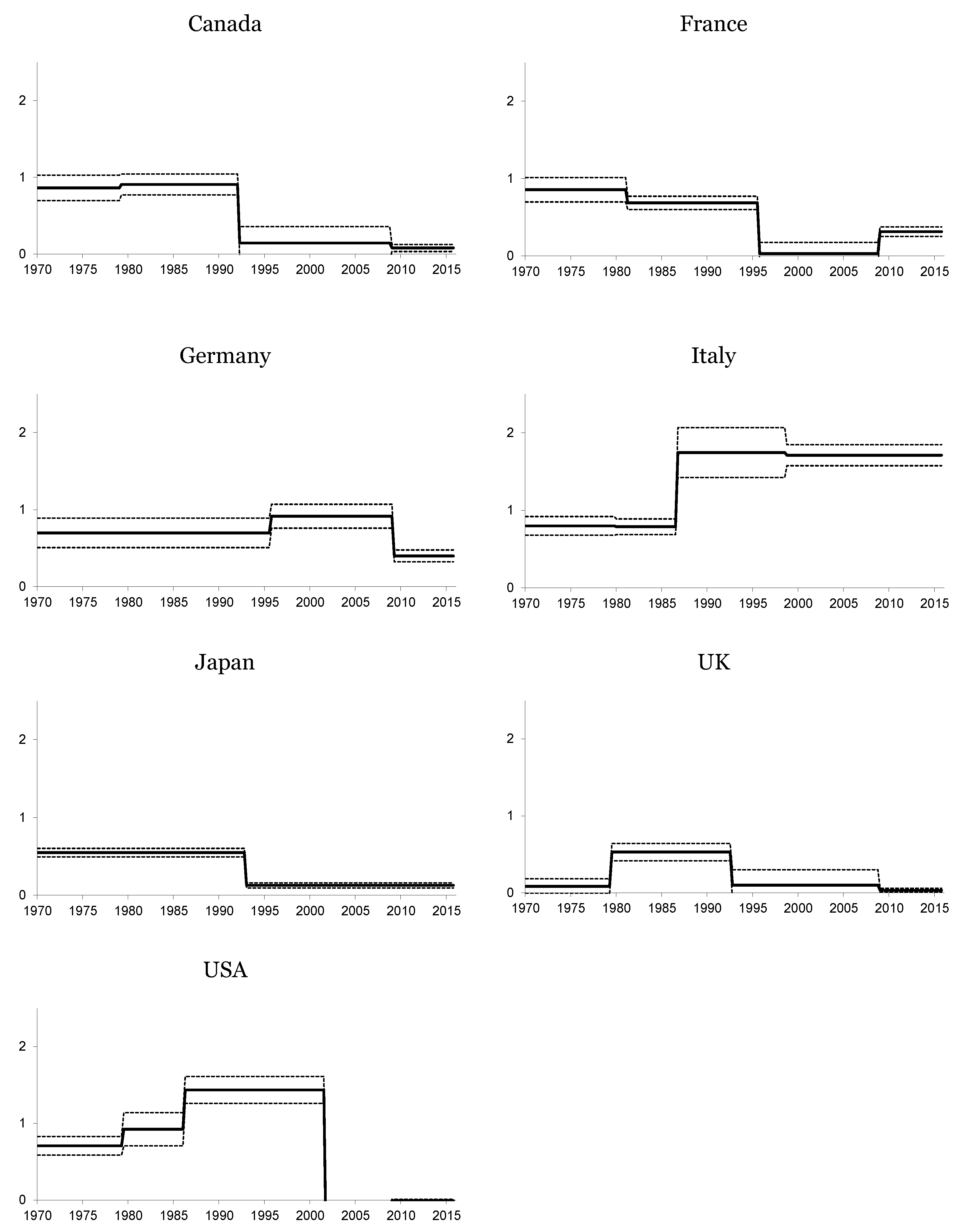
3. Structural Breaks and the Fisher Effect

As we have seen, the presence of a unit root in the variables under examination is not supported by our data. Consequently, we argue that we should test for the Fisher effect by considering that nominal interest rates and inflation rates are not integrated. Malliaropoulos (2000) [14] and Atkins and Chan (2004) [46] tried to provide an appropriate reply to studies of the Fisher effect with stationary variables. These authors first filter the broken trend component for both the nominal interest rate and the inflation rate and then study the relationship between the cyclical components of these two variables. However, we should note that this method does not account for the fact that the presence of breaks may affect the relationship between these variables. To explore this possibility, we can use Bai and Perron’s (1998, 2003) procedure [30,31]. 5 This method allows us to detect the presence of an unknown number of breaks, as well as to estimate the relationship of the Fisher effect. We estimate the following expression, in which up to m breaks may appear:

$$R_t={\alpha }_j+{\beta }_j{\pi }_{t+1}+u_t,t=T{B}_{j-1},\dots .,T{B}_{j}j=1,2,\dots m+1$$

(7)

with $T{B}_j$ representing the period in which the break appears, m representing the number of breaks and $T{B}_o=1$ and $T{B}_{m+1}=T$. The Bai–Perron procedure estimates the above equation by considering that the break may appear in any period of the sample. We then define a Chow-type test in order to determine the existence of a first break, which coincides with the period in which this Chow-type statistic attains its maximum value. We subsequently analyze the existence of multiple breaks by applying this procedure sequentially, combining it with the repartition method described in Bai (1997) [51]. To determine the existence of breaks, we can use the $U{D}_{max}$ and $W{D}_{max}$ statistics, which test the null hypothesis of no structural breaks versus the presence of an unknown number of breaks. Note that we consider a maximum of five breaks and that we use the quadratic spectral kernel to account for the presence of possible autocorrelation and heteroskedasticity in the residuals and the Andrews (1991) [52] automatic bandwidth selection. This method should help us account for the possible dynamic components of the relationship, and consequently, Equation (7) also offers an appropriate scenario in which to test for the Fisher effect from a long-run perspective. The results of this analysis appear in

Table 3. Estimation of the Fisher coefficient.

	${\mathit{WD}}_{\mathit{max}}^{\mathbf{0.05}}$	ψ1	TB1	ψ2	TB2	ψ3	TB3	ψ4	TB4	ψ5	TB5	ψ6
Panel A: long-run nominal interest rates
Canada	616	0.53	79:2	0.61	86:1	0.42	96:3	0.63	07:4	0.18	-	-
France	258	0.61	79:4	1.37	86:3	1.11 $	96:3	0.68	09:1	1.02	-	-
Germany	178	0.40	96:3	0.73	08:4	1.50	-	-	-	-	-	-
Italy	218	0.95	76:3	1.27 $	84:2	1.52	97:2	1.15	-	-	-	-
Japan	1337	0.20	85:2	0.47	95:1	0.07	01:4	0.71	-	-	-	-
UK	495	0.67	76:3	0.13	83:2	0.24	91:3	0.86	98:2	0.07	08:4	0.50
USA	254	0.52	78:4	2.63 $	85:4	0.62	92:2	0.99	00:4	0.12	08:3	0.38
Panel B: short-run nominal interest rates
Canada	642	0.86	79:1	0.89	92:1	0.15	08:4	0.08	-	-	-	-
France	375	0.86 $	81:1	0.68	95:3	0.03	08:4	0.31	-	-	-	-
Germany	185	0.70	95:3	0.92	09:1	0.40	-	-	-	-	-	-
Italy	586	0.80	79:4	0.79	86:3	1.75	98:3	1.71	-	-	-	-
Japan	266	0.55	92:4	0.13	-	-	-	-	-	-	-	-
UK	526	0.08	79:2	0.53	92:3	0.10	08:4	0.03	-	-	-	-
USA	500	0.71	79:2	0.92	86:1	1.43	01:3	−0.70	08:4	−0.01	-	-

This table presents the results of the Bai–Perron procedure and the estimation of the Fisher coefficient for the different estimated regimes. $W{D}_{max}^{0.05}$ ($W{D}_{max}$ at 5% significance level) tests for the null hypothesis of no structural breaks, rejecting this hypothesis for any significance level considered. These statistics have been obtained by correcting the possible autocorrelation/heteroscedasticity by way of the quadratic spectral kernel with the bandwidth being selected according to Andrews (1991) [52]. $TB1,\dots ,TB5$ are the estimated break periods according to the LWZ (modified Schwarz criterion) statistic. ${\psi }_1,\dots ,{\psi }_6$ are the estimations of the Fisher coefficients defined in (8) and (9) for each estimated regime. ^$ means that a second order ARDL (Autoregressive Distributed Lag) model was estimated.

. These results clearly confirm our suspicion of the presence of breaks in the structural relationship between the interest rates and inflation rates. We can verify this by observing the values of $W{D}_{max},$ which clearly reject the null hypothesis of no breaks for almost any level of significance. Thus, it is necessary to consider the presence of these breaks in order to reflect this relationship appropriately.

The findings of this study contribute to different debates with respect to the relationship between nominal rates and expected inflation. First, previous research highlighted the importance of the term structure of interest rates because it contains some information to forecast inflation (Fama (1990) [53]). Furthermore, by using short-run interest rates, we only observe a liquidity effect instead of the Fisher relationship. Fahmy and Kandil (2003) [54] conclude that the ability of nominal interest rates to capture inflationary expectations increases with maturity, attaining a one-to-one relationship for assets of five-year maturity. On the other hand, numerous studies, including that of Fisher himself, test the Fisher effect using short-run interest rates (e.g., Mishkin (1992) [5] and Evans and Lewis (1995) [55]).

In this framework, we find some significant differences in the results using short- and long-term interest rates. First, we can see that the number of breaks is greater when using the long-run rather than the short-run nominal interest rate. This can be interpreted by considering that the short-run interest rates react more quickly than the long-run interest rates to the changes in the inflation. We can also observe that there is some coincidence with respect to the estimation of the periods in which the breaks appear and, of special interest, the break related to the Great Recession.

We can now analyze the estimation results for the β parameter, which determines whether the Fisher effect holds. To that end, instead of using the estimated Equation (7), it seems to be much more appropriate to split the sample by using the estimated breaks and, then, to include some lags in the specification to better capture the dynamics of the relationship by way of an ARDL (Autoregressive Distributed Lag) of order one.

$$R_t={\alpha }_j+{\beta }_j{\pi }_{t+1}+{\gamma }_j{R}_{t-1}+{\varphi }_j{\pi }_t+u_t,t=T{B}_{j-1}+2,\dots .,T{B}_{j}j=1,\dots m+1$$

(8)

and, subsequently, obtain the long-run multiplier for the Fisher coefficient defined as:

$${\psi }_j=\frac{{\beta }_j+{\varphi }_j}{1-{\gamma }_j}$$

(9)

We should note that the effective sample removes the initial observations of each segment in order to assure that all of the information belongs to the same estimated period. Later, we use bootstrap methods based on 1000 replications to obtain the confidence intervals of the estimated ψ. Figure 2 and Figure 3 present the results for the long- and short-run nominal interest rates, respectively.

We can first observe that there is a clear relationship between interest rates and expected inflation, although the estimated coefficients are some distance from unity, and therefore, the transmission of the effect from expected inflation rates to interest rates is not exactly the one predicted by the Fisher effect. Moreover, we can frequently reject the null hypothesis that the ${\psi }_j$ coefficients are equal to one, thus failing to provide evidence of the Fisher effect for most periods of the sample. Therefore, we can broadly conclude that there is a weak Fisher effect or, in other words, that the nominal interest rate “under-adjusts” to a change in inflation evolution, and consequently, a transmission to real rates exists.

This is a crucial issue in macroeconomics and monetary economics because it implies rejecting superneutrality. This hypothesis holds if changes in the money supply affect inflationary expectations and, in turn, real rates. In the absence of a full Fisher effect, shocks to inflation would translate into disturbances in real rates, which is a controversial result in the context of standard models of inter-temporal asset pricing and would break monetary neutrality. However, our estimation results show a link between nominal rates and expected inflation, but not the required full one-to-one adjustment of the former to the latter. Rapach and Wohar (2005) [56] obtain similar results.

Many studies propose explanations of the lack of empirical evidence of the Fisher hypothesis. Together with the inability to measure inflationary expectations directly, the Mundell–Tobin effect emerges as the most likely theoretical explanation for a β coefficient less than one, in accordance with the results in Table 2. Following the Tobin (1965) [57] formulation, agents replace nominal assets for real money balances in response to increases in expected inflation. This reallocation process increases capital stock and lowers the long-run real return to capital. In Mundell’s (1963) model [58], an increase in inflation raises savings if they depend on a real money balance, via the wealth effect, and thus, the real interest rate falls. Accordingly, the Mundell–Tobin effect predicts a negative long-run real interest rate response to an increase in inflation, and thus, the nominal interest rate would rise by less than unity. 6

By assuming some degree of inflationary monetary transmission to real interest rates, it is interesting to study the influence of changes in monetary policy on the Fisher effect. Using a dynamic expectations model with staggered price-setting, Söderling (2001) [29] claims that a more active monetary policy decreases the Fisher effect. This finding has been supported in the well-documented case of the USA. Numerous studies (e.g., Miskhin (1992) [5] and Lanne (2001) [15]) find strong evidence supporting the Fisher hypothesis for the period between the early 1950s to 1979, characterized by interest rate targeting while the Federal Reserve was especially concerned with growth and the employment level. On the other hand, the effect is absent in the post-1970 sub-sample periods when monetary policy emphasized inflation targeting.

The analysis of the periods in which the breaks appear provides some rich insights. We can see that the most common breaks appear in four fairly well-defined periods: in the late 1970s, in the mid-1980s, in the mid-1990s and, finally, in the second part of the 2000s, clearly related to the Great Recession. 7 The periods in which the breaks appear can be easily interpreted from an economic point of view. The first and second breaks are connected with the general tightening of monetary policy applied with different rhythms in each country. The case of the USA, where the Federal Reserve introduced new operational procedures in 1979 and the inflation target gained weight in its reaction function, is a good example. 8 The third break is not connected with a single cause; rather, its origin may be related to multiple causes because it coincides with a somewhat convulsive period as far as monetary policy is concerned. For instance, we should consider that the crisis of the European Monetary System occurred during that period. Therefore, it comes as no surprise that the estimation of this break is less accurate than the estimation of the other breaks. However, and despite some occasional episodes, monetary policy in the 1990s tended towards more stability and greater credibility of central banks that maintained their inflation targets. Finally, the recent international crisis is clearly behind the last period.

If we analyze the estimations of the β coefficients from a historical perspective, some further insights emerge. We begin with the long-run equation in which we can see that the estimated values of the β coefficients for the first regime are lower than one. Italy exhibits the highest value (0.95) and Japan the lowest value (0.20). The rest of the estimated coefficients are around 0.5, clearly rejecting the Fisher hypothesis.

Interestingly, we can also appreciate that the first oil crisis does not seem to affect the Fisher equation, despite the fact that this phenomenon clearly affected inflation in all of the countries included in our study. Moreover, some previous studies, such as that of Rapach and Wohar (2005) [56], detect a break for the real interest rate in industrialized countries in 1973. Therefore, according to our results, the increase in the inflation rate during that period was absorbed by the movements in the nominal interest rates and, consequently, the Fisher relationship remained unaltered.

The second period covers the years running from the late 1970s to the mid-1980s. The most noteworthy economic event of this time was the change in monetary policy, which became more restrictive. The main finding associated with this period is the increase in the estimated value of the coefficients, especially remarkable for France and the USA and much more moderate for Canada and Italy. The evolution of the Fisher coefficient during the 1990s and 2000s shows a downward path for France, the USA and, to a lesser extent, the UK, whilst Germany, Japan and Italy show slight increases. In any event, except for the case of Italy, the value of this coefficient is well below one. Finally, the effect of the Great Recession implies a clear increase in this parameter for France and Germany, in excess of one. These increases are much more moderate for the UK, Japan and the USA.

Let us now consider the short-run model. The estimated values of the Fisher parameter are not globally distant from those of the long-run model, being quite similar to or slightly higher than those up to the 2000s, but showing a clear decline in the final part of the sample. We can thus conclude that the values of the expected inflation rates are again transmitted to short-run nominal interest rates for the sample countries. Note, however, that the amount transmitted is below the value predicted by the Fisher hypothesis and is slightly slower than that transmitted to the long-run nominal interest rates, especially after the Great Recession. The exception to this behavior is Italy, which exhibits a somewhat stable value of more than one for this coefficient.

We can also see that the estimated values of the β coefficients show an upward trend from the beginning of the sample to the mid-1990s. Finally, we can observe that the estimated value of the β coefficient exhibits a clear reduction from the mid-1990s onwards, especially noticeable after the Great Recession. Thus, the expected inflation rate does not act as a good predictor of the short-run nominal interest rates during this period. This situation is quite understandable for the EU countries, which lost their independence in terms of monetary policy following the introduction of the euro and the fixing of nominal interest rates by the European Central Bank. The Japanese results can be explained by the substantial reduction in the nominal interest rates that aimed to re-activate the economy. This makes it easy to explain why the estimated values of both the intercept and the β coefficient decreased since the 1990s. By contrast, the transmission of the expected inflation to nominal interest rates remained virtually unaltered in the USA. In short, the Fisher effect seems to decrease, and nearly disappear, in the 1990s, coinciding with more stable inflation expectations because central banks halted price pressures in the economy to meet their inflation targets. As a result, the nominal and real interest rates move in parallel.

4. Conclusions

In this study, we offer evidence of the fact that the nominal interest rates and inflation rates of the G7 group of countries are better characterized as I(0) variables than as first order integrated variables. We obtain this conclusion by using recently developed panel data unit root tests. Consequently, we should note that using techniques based on unit root/co-integration tests should be carefully reconsidered when analyzing the relationship between nominal interest rates and inflation rates, which are commonly studied by estimating the Fisher equation.

We also considered the presence of some breaks in the Fisher equation in order to capture the different monetary regimes that co-exist across the sample. Using a procedure recently proposed in Bai and Perron (1998, 2003) [30,31] confirms our hypothesis, offering robust evidence of the existence of different regimes in the relationship between nominal interest rates and inflation rates.

This procedure also offers an excellent scenario for testing for the Fisher effect, considering the presence of breaks in the relationship that affects both parameters. The results based on this method show that there is a clear connection between nominal interest rates and expected inflation rates. However, there is no evidence of a total Fisher effect for the G7 countries. Inflation is not always transmitted to nominal interest rates. In fact, we should note that the Fisher coefficient estimates have very high variations. The changes in the monetary policy produced an adjustment in the transmission of the effect of inflation to nominal interest rates.

We also observed the existence of four different regimes in the relationship between nominal interest rates and expected inflation rates in the estimated periods, in which the regimes changed during the late 1970s, mid-1980s, mid-1990s and the late 2000s. It is remarkable to notice that there is no break associated with the first oil crisis (around 1973), despite the fact that previous studies analyzing real interest rates offered evidence of a break at that time. We should nevertheless note that these studies consider that the β coefficient of the Fisher equation is equal to one, a value that is consistently rejected for most of the cases analyzed in the present study.

Finally, we observed that the transmission of the expected inflation to nominal interest rates was greater in Italy than in the other countries and was very low in Japan, the UK and Canada. France, the USA and Germany also showed periods with a significant transmission of the inflation rates to nominal interest rates, even exceeding the value of one.

To sum up, our findings show that regime changes govern the Fisher equation. The estimations show a link between nominal interest rates and expected inflation, but a weak Fisher effect, which does not support the monetary neutrality hypothesis. The values obtained for the Fisher coefficients lead us to conclude that there is “under-adjustment” of nominal rates to inflationary expectations and, consequently, of their transmission to real rates. Furthermore, as stated above, the weakness of the Fisher effect increases with the credibility of monetary policy.

References

1. I. Fisher. The Theory of Interest. New York, NY, USA: MacMillan, 1930. [Google Scholar]
2. G.M. Caporale, and N. Pittis. “Estimator Choice and Fisher’s Paradox: A Monte Carlo Study.” Econom. Rev. 23 (2004): 25–52. [Google Scholar] [CrossRef]
3. E. Panopoulou. “A Resolution of the Fisher Effect Puzzle: A Comparison of Estimators.” IIIS Discussion Paper, 67. 2005. Available online: https://ssrn.com/abstract=680401 (accessed on 15 July 2016).
4. A.K. Rose. “Is the Real Interest Rate Stable? ” J. Financ. 43 (1988): 1095–1112. [Google Scholar] [CrossRef]
5. F. Mishkin. “Is the Fisher effect for real: A Reexamination of the Relationship between Inflation and Interest Rates.” J. Monetary Econ. 30 (1992): 195–215. [Google Scholar] [CrossRef]
6. W.J. Crowder, and M.E. Wohar. “Are Tax Effects Important in the Long-Run Fisher Relationship? Evidence from the Municipal Bond Market.” J. Financ. 54 (1992): 307–317. [Google Scholar] [CrossRef]
7. Z. Koustas, and A. Serletis. “On the Fisher Effect.” J. Monetary Econ. 44 (1999): 105–130. [Google Scholar] [CrossRef]
8. D.E. Rapach. “The Log-run Relationship between Inflation and Real Stock Price.” J. Macroecon. 24 (2004): 331–351. [Google Scholar] [CrossRef]
9. F. Laatsch, and D.P. Klein. “Nominal Interest Rate and Expected Inflation: Results from a Study of US Treasury Inflation-Protected Securities.” Q. Rev. Econ. Financ. 43 (2003): 3405–3417. [Google Scholar] [CrossRef]
10. D.E. Rapach, and C. Weber. “Are Real Interest Rates Really Nonstationary? New Evidence from Tests with Good Size and Power.” J. Macroecon. 26 (2005): 409–430. [Google Scholar] [CrossRef]
11. J. Westerlund. “Panel cointegration tests of the Fisher effect.” J. Appl. Econom. 23 (2008): 193–233. [Google Scholar] [CrossRef]
12. B. Ozcan, and A. Ari. “Does the Fisher hypothesis hold for the G7? Evidence from the panel cointegration test.” Econ. Res.-Ekon. Istraz. 28 (2015): 271–283. [Google Scholar] [CrossRef]
13. J.C. Cox, J.E. Ingersoll, and S.A. Ross. “A theory of the term structure of interest rates.” Econometrica 53 (1985): 385–407. [Google Scholar] [CrossRef]
14. D. Malliaropulos. “A Note on Nonstationarity, Structural Breaks and the Fisher Effect.” J. Bank. Financ. 24 (2000): 695–707. [Google Scholar] [CrossRef]
15. M. Lanne. “Near Unit Root and the Relationship between Inflation and Interest Rate: A Reexamination of the Fisher Effect.” Empir. Econ. 26 (2001): 357–366. [Google Scholar] [CrossRef]
16. N. Olekalns. An Empirical Investigation of the Structural Breaks in the Ex Ante Fisher Effect. Research Paper Number 786; Melbourne, Australia: Department of Economics, University of Melbourne, 2001. [Google Scholar]
17. L.A. Gil-Alaña. “A Mean Shift Break in the US Interest Rate.” Econ. Lett. 77 (2002): 357–363. [Google Scholar] [CrossRef]
18. F.J. Atkins, and P.J. Coe. “An ARDL Bounds Test of the Long-term Fisher Effect in the United States and Canada.” J. Macroecon. 24 (2002): 255–266. [Google Scholar] [CrossRef]
19. C.F. Baum, J.T. Barkoulas, and M. Caglayan. “Persistence in International Inflation Rates.” South Econ. J. 65 (1999): 900–913. [Google Scholar] [CrossRef]
20. P. Phillips, and P. Perron. “Testing for a Unit Root in Time Series Regression.” Biometrika 75 (1988): 335–346. [Google Scholar] [CrossRef]
21. W.J. Tsay. “The long memory story of the real interest rate.” Econ. Lett. 67 (2000): 325–330. [Google Scholar] [CrossRef]
22. X. Sun, and P.C.B. Phillips. “Understanding the Fisher Equation.” J. Appl. Econom. 19 (2004): 869–896. [Google Scholar] [CrossRef]
23. L.A. Gil-Alaña. “Estimation of the order of integration in the UK and the US interest rates using fractionally integrated semiparametric techniques.” Eur. Res. Stud. 7 (2004): 29–40. [Google Scholar]
24. L.A. Gil-Alaña, and A. Moreno. “Fractional integration and structural breaks in U.S. macro dynamics.” Empir. Econ. 43 (2012): 427–446. [Google Scholar] [CrossRef]
25. U. Hassler, and J. Wolters. “Long Memory in Inflation Rates: International Evidence.” J. Bus. Econ. Stat. 13 (1995): 37–45. [Google Scholar] [CrossRef]
26. C.S. Bos, P.H. Franses, and M. Ooms. “Long Memory and Level Shifts: Reanalysing Inflation Rates.” Empir. Econ. 24 (1999): 427–449. [Google Scholar] [CrossRef]
27. R.E. Lucas Jr. “Econometric Policy Evaluation: A Critique.” Carnegie-Rochester Conf. Ser. Public Policy 2 (1976): 19–46. [Google Scholar] [CrossRef]
28. J.S. Chadha, and N.H. Dimsdale. “A Long Review of Real Rates.” Oxf. Rev. Econ. Policy 15 (1999): 17–45. [Google Scholar] [CrossRef]
29. P. Söderlind. “Monetary Policy and the Fisher Effect.” J. Policy Model. 23 (2001): 491–495. [Google Scholar] [CrossRef]
30. J. Bai, and P. Perron. “Estimating and Testing Linear Models with Multiple Structural Changes.” Econometrica 66 (1998): 47–78. [Google Scholar] [CrossRef]
31. J. Bai, and P. Perron. “Computation and analysis of multiple structural-change models.” J. Appl. Econom. 18 (2003): 1–22. [Google Scholar] [CrossRef]
32. C.R. Nelson, and C.I. Plosser. “Trends and Random Walks in Macroeconomic Time Series: Some Evidence and Implications.” J. Monetary Econ. 10 (1982): 139–162. [Google Scholar] [CrossRef]
33. D. Dickey, and W. Fuller. “Distribution of the Estimators for Autoregressive Time Series with a Unit Root.” J. Am. Stat. Assoc. 74 (1979): 427–431. [Google Scholar] [CrossRef]
34. S.E. Said, and D. Dickey. “Testing for Unit Roots in Autoregressive-Moving Average Models of Unknown Order.” Biometrika 71 (1984): 599–607. [Google Scholar] [CrossRef]
35. S. Ng, and P. Perron. “Lag Length Selection and the Construction of Unit Root Tests With Good Size and Power.” Econometrica 69 (2001): 1519–1554. [Google Scholar] [CrossRef]
36. G. Elliot, T.J. Rothenbert, and J.H. Stock. “Efficient tests for an autoregressive unit root.” Econometrica 64 (1996): 813–836. [Google Scholar] [CrossRef]
37. M.H. Pesaran. “General Diagnostic Tests for Cross Section Dependence in Panels.” IZA Discussion Paper 1240. 2004. Available online: http://www.econ.cam.ac.uk/research/repec/cam/pdf/cwpe0435.pdf (accessed on 1 August 2016).
38. M.H. Pesaran. “A simple panel unit root test in the presence of cross-section dependence.” J. Appl. Econom. 22 (2007): 265–312. [Google Scholar] [CrossRef]
39. M.H. Pesaran. “Testing Weak Cross-Sectional Dependence in Large Panels.” IZA Discussion Paper 6432. 2012. Available online: http://ftp.iza.org/dp6432.pdf (accessed on 1 August 2016).
40. M. Costantini, and C. Lupi. “An analysis of inflation and interest rates. New panel unit root results in the presence of structural breaks.” Econ. Lett. 95 (2007): 408–414. [Google Scholar] [CrossRef]
41. C.C. Lee, and C.P. Chang. “Mean reversion of inflation rates in 19 OECD countries: Evidence from panel Lm unit root tests with structural breaks.” Econ. Bull. 3 (2007): 1–15. [Google Scholar]
42. C.C. Lee, and C.P. Chang. “Trend stationary of inflation rates: Evidence from LM unit root testing with a long span of historical data.” Appl. Econ. 40 (2008): 2523–2536. [Google Scholar] [CrossRef]
43. J. Lee, and M. Strazicich. “Minimum LM Unit Root Tests with Two Structural Breaks.” Rev. Econ. Stat. 40 (2003): 1082–1089. [Google Scholar] [CrossRef]
44. J. Lee, and M. Strazicich. “Minimum LM Unit Root Test.” Econ. Bull. 33 (2013): 2483–2492. [Google Scholar]
45. M.D. Gadea, A. Montañés, and M. Reyes. “The European Union Currencies and the US Dollar: From post-Bretton-Woods to the Euro.” J. Int. Money Financ. 23 (2004): 1109–1136. [Google Scholar] [CrossRef]
46. F.J. Atkins, and M. Chan. “Trend breaks and the Fisher Hypothesis in Canada and the United States.” Appl. Econ. 36 (2004): 1907–1913. [Google Scholar] [CrossRef]
47. R. Garcia, and P. Perron. “An Analysis of the Real Interest Rate under Regime Shifts.” Rev. Econ. Stat. 78 (1996): 111–125. [Google Scholar] [CrossRef]
48. H.J. Bierens. “Nonparametric Nonlinear Co-Trending Analysis, with an Application to Inflation and Interest in the U.S.” J. Bus. Econ. Stat. 18 (2000): 323–337. [Google Scholar]
49. M. Lanne. “Nonlinear dynamics of interest and inflation.” J. Appl. Econom. 21 (2006): 1157–1168. [Google Scholar] [CrossRef]
50. E. Panopoulou, and T. Pantelidis. “The Fisher effect in the presence of time-varying coefficients.” Comp. Stat. Data Anal. 100 (2016): 495–511. [Google Scholar] [CrossRef]
51. J. Bai. “Estimation of a Change Point in Multiple Regression Models.” Rev. Econ. Stat. 79 (1997): 551–563. [Google Scholar] [CrossRef]
52. D.W.K. Andrews. “Heteroskedasticity and Autocorrelation Consistent Covariance Matrix Estimation.” Econometrica 59 (1991): 817–858. [Google Scholar] [CrossRef]
53. E.F. Fama. “Term structure forecast of interest rates, inflation and real returns.” J. Monetary Econ. 25 (1990): 59–76. [Google Scholar] [CrossRef]
54. Y.A.F. Fahmy, and M. Kandil. “The Fisher effect: New evidence and implications.” Int. Rev. Econ. Financ. 12 (2003): 451–465. [Google Scholar] [CrossRef]
55. M. Evans, and K. Lewis. “Do expected shifts in inflation affect estimates of the long-run Fisher relation? ” J. Financ. 50 (1995): 225–253. [Google Scholar] [CrossRef]
56. D.E. Rapach, and M.E. Wohar. “Regime Changes in International Real Interest Rates: Are They a Monetary Phenomenon? ” J. Money Credit Bank. 37 (2005): 887–906. [Google Scholar] [CrossRef]
57. J. Tobin. “The interest-elasticity of transactions demand for cash.” Rev. Econ. Stat. 38 (1956): 241–247. [Google Scholar] [CrossRef]
58. R. Mundell. “Inflation and Real Interest.” J. Polit. Econ. 71 (1963): 280–283. [Google Scholar] [CrossRef]
59. D.E. Rapach. “International Evidence on the Long-run Impact of Inflation.” J. Money Credit Bank. 33 (2003): 23–48. [Google Scholar] [CrossRef]
60. R. Clarida, J. Galí, and M. Gertler. “Monetary policy rules and macroeconomic stability evidence and some theory.” Q. J. Econ. 115 (2000): 147–180. [Google Scholar] [CrossRef]
Figure 1. (a) Expected Inflation rates; (b) Long-run nominal interest rates; (c) Short-run nominal interest rates.
Econometrics 05 00011 g001aEconometrics 05 00011 g001bEconometrics 05 00011 g001c
Figure 2. Estimated Fisher Coefficient. Long-run nominal interest rate. The solid line represents the estimated Fisher coefficient defined by (9), whilst the dotted line reflects twice the standard deviation, obtained by way of bootstrapping techniques.
Econometrics 05 00011 g002
Figure 3. Estimated Fisher Coefficient. Short-run nominal interest rate. The solid line represents the estimated Fisher coefficient defined by (9), whilst the dotted line reflects twice the standard deviation, obtained by way of the bootstrapping techniques.
Econometrics 05 00011 g003