Stable-GARCH Models for Financial Returns: Fast Estimation and Tests for Stability

Abstract

A fast method for estimating the parameters of a stable-APARCH not requiring likelihood or iteration is proposed. Several powerful tests for the (asymmetric) stable Paretian distribution with tail index $1<\alpha <2$ are used for assessing the appropriateness of the stable assumption as the innovations process in stable-GARCH-type models for daily stock returns. Overall, there is strong evidence against the stable as the correct innovations assumption for all stocks and time periods, though for many stocks and windows of data, the stable hypothesis is not rejected.

1. Introduction

Since the seminal work of Mandelbrot [1] and Fama [2], the stable Paretian distribution for modeling financial asset returns has generated increasing interest, as computer power required for its computation became commonplace, and given its appealing theoretical properties of (i) summability (as can be used for portfolio analysis; see [3,4,5], and the references therein); (ii) its heavy tails and asymmetry that are ubiquitously characteristic of financial asset returns; and (iii) it being the limiting distribution of sums of various independent identically distributed (i.i.d.) random variables, i.e., such sums are in the domain of attraction of a stable law; see, e.g., Geluk and De Haan [6] and the references therein. McCulloch [7], Rachev and Mittnik [8], Borak et al. [9], and Nolan [10] offer extensive accounts of the stable distribution and its wide applicability in finance, while Samorodnitsky and Taqqu [11] provides a more technical development including the multivariate setting. Extensions and compliments to the use of the stable Paretian include the tempered stable (see e.g., [12,13], and the references therein) and the geometric stable (see, e.g., [14,15,16], and the numerous references therein).

As asset returns measured at the weekly, daily, or higher frequency exhibit the near-immutable property of conditional heteroskedasticity, GARCH-type models are employed when interest centers on short-term density and risk prediction. While such models, driven by Gaussian innovations, result in a heavy-tailed process (see [17,18,19,20]; and the references therein), the residuals themselves are still highly non-Gaussian, and numerous suggestions have been made for replacing the Gaussian distribution with a leptokurtic one, the seminal article being Bollerslev [21] with the use of a Student’s t. Owing to computational advances, the stable distribution was subsequently used; see [22,23,24] for details of this model, its computation based on maximum likelihood, and the stationarity conditions.

In this paper, we propose two estimation methods. The first is based on traditional use of the MLE, and focuses on a new, efficient, vectorized evaluation of the stable density. The second is a very different and new estimation methodology for the stable-GARCH model that is extremely fast, as it does not require evaluation of the likelihood or numerical optimization methods.

Given (i) the appealing theoretical properties of the stable distribution; (ii) the fact that the expected shortfall (ES) risk measure, as a left tail partial first moment ($\mathbb{E}[X\mid X\le c]$, where c is the VaR), is potentially highly dependent on the distributional assumption (see [25,26], and the references therein); and (iii) that ES is not elicitable and thus more difficult to empirically test compared to VaR (see [27]), one is motivated to test the validity of the stable Paretian assumption as the innovations sequence for a GARCH-type model used for risk prediction or asset allocation.

Testing the stable Paretian distribution has been considered by several authors. Koutrouvelis and Meintanis [28], Meintanis [29], and Matsui and Takemura [30] use the empirical characteristic function to develop testing procedures in the symmetric stable case. Fama and Roll [31], Lau and Lau [32], and Paolella [33,34] consider the change in the estimated tail index, α, as the data are summed: If the data are stable, then the value of α should not change, whereas for many alternatives outside the stable class, the classic central limit theorem will be at work, and the values of α will tend to increase towards two as the data are summed. McCulloch and Percy [35] propose a set of composite (unknown parameter case) tests for, among others, the symmetric stable distribution and are able to reject the null in their applications, though they attribute this primarily to the presence of asymmetry.

Paolella [34] also proposes a test based on the difference of two consistent estimators of the tail index α, and combines this with a new summability test, termed $A+{\tau }_{20}$, yielding a test that is (i) size correct; (ii) often substantially more powerful than either of its two constituents and much more powerful than the test based on the empirical characteristic function; (iii) easily computed, without the need for the density or maximum likelihood (ML) estimation of the stable distribution; (iv) applicable in the asymmetric case; and (v) also delivers an approximate p-value.

Our second interest in this paper is to use some of these tests applied to the filtered innovations sequences of stable-GARCH models, in an effort to determine the applicability of the stable assumption as the underlying distribution. While the literature is rich in proposing various GARCH-type models with a variety of distributional assumptions on the innovations process, there is not as much work dedicated to testing such assumptions. Klar et al. [36] propose use of a characteristic function based test applied to the filtered residuals and use a bootstrap to assess small-sample properties; and also contains references to some earlier literature for GARCH distributional testing.

Of interest in such a testing framework are the results of Sun and Zhou [37], which demonstrate that, as the normal-GARCH process approaches the IGARCH border, the filtered innovation sequence could exhibit artificially heavier tails. Recall that, in classic time series literature, it is known that, if an AR(1) model is misspecified and the true process contains time-varying parameters or structural breaks, then, as the sample size increases, the probability of unit-root tests not rejecting the null of a unit root often increases; see, e.g., Kim et al. [38] and the references therein. Similarly, in a GARCH context, under certain types of misspecification, as the sample size increases, the fitted GARCH model will tend to the IGARCH border as the sample size increases. We attempt to counteract this phenomenon by (i) using short windows of data; (ii) fit the rather flexible stable-APARCH model, as opposed to appealing to quasi-maximum likelihood, which uses a normality assumption on the error term in the GARCH process; and (iii) investigate results when imposing a fixed APARCH structure which is not close to the IGARCH border; see Section 5.3 below, and, in particular, the discussion of the use of (18). In this way, the (in general, highly relevant) findings of Sun and Zhou [37] are less applicable to our setting.

Anticipating our empirical results below, we find that, for most stocks and numerous segments of time, the assumption of the innovation process driving a GARCH-type process being i.i.d. asymmetric stable Paretian cannot be rejected. However, when viewing all the resulting p-values, they follow more of an exponential-type distribution rather than a uniform, and thus there is substantial evidence against the stable as the correct distribution for all stocks and time periods.

The remainder of this paper is structured as follows. Section 2 discusses and refutes the common argument against using the stable distribution for modeling financial asset returns. Section 3 briefly introduces the stable distribution and methods for its computation and estimation, while Section 4 details the tests for the symmetric and asymmetric stable Paretian assumption. Section 5 discusses two new methods for estimating a stable-APARCH process and also provides a comparison with the competitive method of estimation based on the characteristic function, in the i.i.d. setting. Section 6 provides simulation evidence under the true model and some deviations from it, to illustrate the behavior of the model parameter estimates and test statistics. Section 7 provides an empirical illustration, applying the tests to the filtered innovations sequences of the fitted stable-APARCH process to the constituents of the DJIA-30 and the 100 largest market-cap stocks from the S&P500 index. Section 8 provides concluding remarks concerning distributional choices for modeling asset returns and the role of testing.

2. Critique of the Stable Paretian Assumption

The primary argument invoked by some against use of the stable Paretian distribution in a financial context is that (except in the special case of the Gaussian), the second moment, i.e., the variance, does not exist. We wish to dismantle this concern. There indeed exists literature, influential papers including Loretan and Phillips [39], that provide evidence of the existence of second moments in financial data. The problem with all such attempts at inference in this regard is that the determination of the maximally existing moment of a set of data is notoriously difficult; see McCulloch [40], Mittnik et al. [41], McNeil et al. [42], Heyde and Kou [43], and the references therein for critique of such studies.

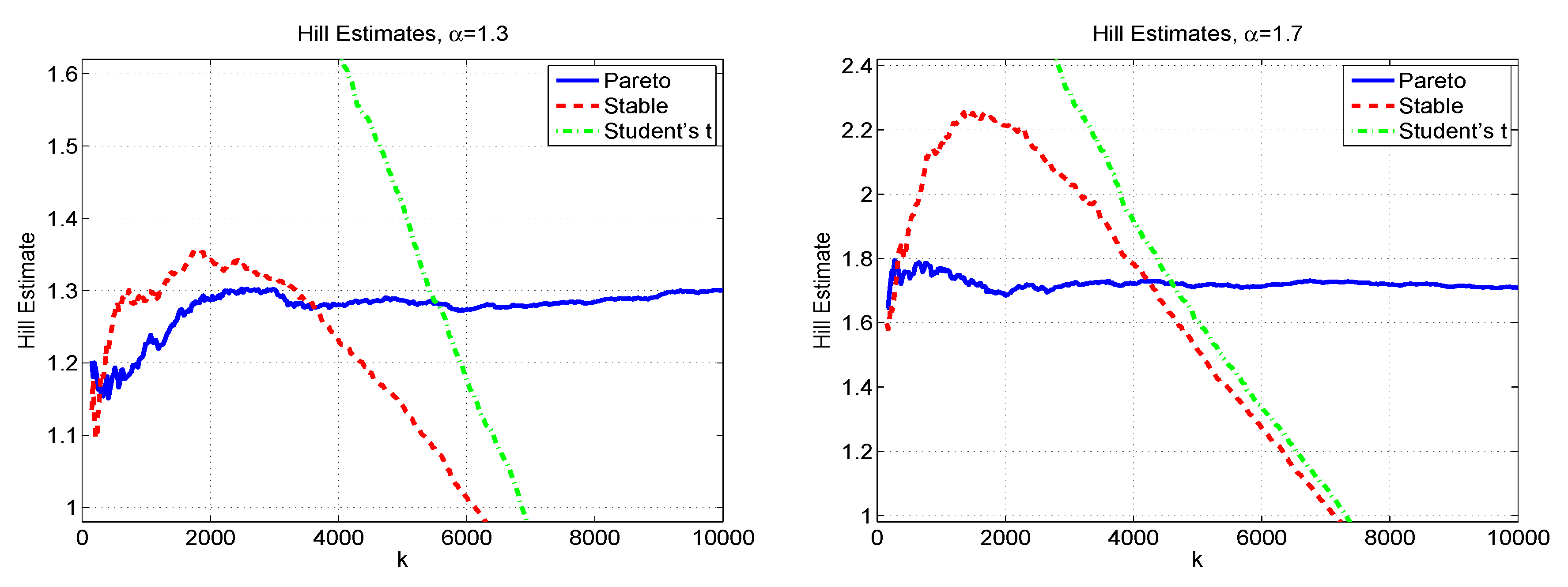
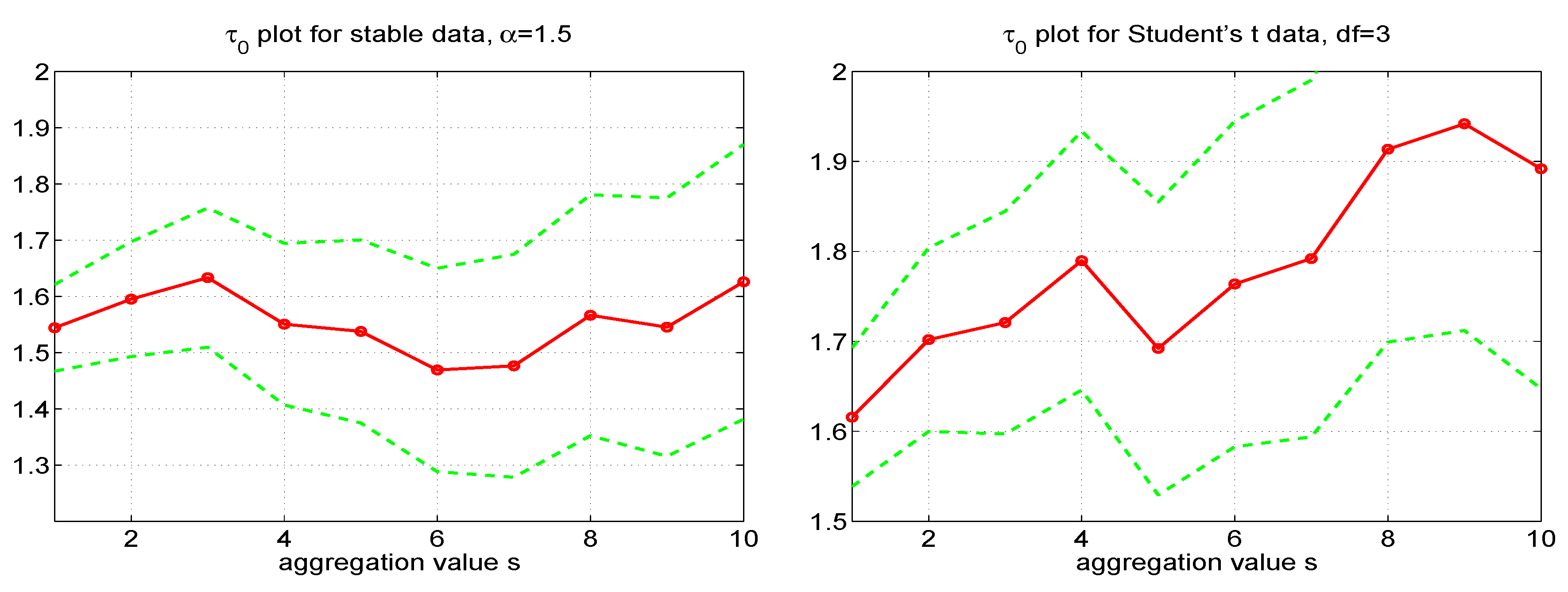
It should be noted that non-existence of variance cannot be claimed if a fitted stable distribution has a tail index, α, whose confidence interval (easily computed nowadays via a parametric or nonparametric bootstrap) does not contain the upper value of two. The flaw is that, first, an entire parametric assumption is being placed on the density, whereas interest centers only on the tails; and second, this particular parametric structure enforces non-existence of variance except in the measure-zero case of normality. As an example, using a reasonably sized set of simulated Student’s t data with degrees of freedom $v=4$ (implying the supremum of the existing moments is four) and fitting a (location-scale) stable distribution will result in an estimated tail index of around $\alpha =1.7$, and whose confidence intervals do not include two. The conclusion that the variance does not exist is false.

Going the other way, if simulated stable Paretian data with $\alpha =1.7$ are fit with a (location-scale) Student’s t model, the estimated degrees of freedom will be around 4, and such that confidence intervals often do not extend below two. The conclusion that the variance exists is false. This disparity of the actual tail index, when estimated via a parametric structure, is, again, an artefact of imposing a parametric heavy tailed density such that the tail index is bound between 0 and 2, and at two, the distribution becomes the Gaussian. This mapping is continuous (e.g., for α close to 2, the density is indeed “close to” Gaussian, except in the extreme tails). As such, the use of these and related parametric models is not justified for inference about the maximally existing moment in the absence of a strict parametric assumption.

It is important to emphasize that, if the data are non-Gaussian stable, then the traditional measures of asymmetry and heavy-tails vis sample skewness ${\widehat{\mu }}_3$ (as the scale-standardized third central moment) and kurtosis ${\widehat{\mu }}_4$ (as the fourth), respectively, are not valid, because their theoretical counterparts do not exist. As such, while an empirically computed sample kurtosis will be large, the law of large numbers is not applicable, and it will not converge as the sample size increases. This is not the case with Student’s t data with degrees of freedom, v, larger than four. In that case, the sample kurtosis is informative for estimation of v. For example, Singh [44] proposed an estimator of v, assuming $v>4$, as $\widehat{v}=2(2{\widehat{\mu }}_4-3){({\widehat{\mu }}_4-3)}^{-1}$.

It is noteworthy that there do exist periods of stock returns and indexes, particularly during crisis periods, such that not only is the tail index of the stable far less than two, but also even the Student’s t fit yields estimated tail indices below two. While this is still not a formal test of non-existence of second moments, it does provide strong evidence that that existence of the variance can be questioned. Observe that traditional methods of portfolio optimization, which make use of the sample variance-covariance matrix of returns data, would then be invalid; see, e.g., Gamba [3]. This is addressed, for example, in Giacometti et al. [4], Doganoglu et al. [5], Paolella [45], Paolella and Polak [46], and the references therein.

The existence of moments is determined from the asymptotic tail behavior, but in practical applications, there are never enough data points to accurately characterize the tail. This point is forcefully made in Heyde and Kou [43]. This helps explain why models using distributions with completely different tail behaviors all can perform very well in terms of value at risk (VaR) forecasting, this being a left-tail quantile of the predictive returns distribution of a portfolio of assets.

For example, Haas et al. [47], Alexander and Lazar [48], Haas et al. [49], Haas and Paolella [50] and Haas et al. [51] use discrete normal mixture (MixN) GARCH models, with the MixN being a short-tailed distribution; Broda and Paolella [52] use a normal inverse Gaussian (NIG) structure, this having so-called semi-heavy tails (and existence of a moment generating function); several authors, including Mittnik and Paolella [53], Kuester et al. [54], and Krause and Paolella [55] use an asymmetric Student’s t distribution (this having heavy tails but such that the tail index lies in $(0,\infty )$); Mittnik and Paolella [56] and Broda et al. [57] use the asymmetric stable and mixtures of symmetric stable, respectively, these having heavy tails such that the tail index lies in $(0,2)$. The fact that all of these methods can deliver highly accurate VaR forecasts confirms that the choice of asymptotic tail behavior and the (non-)existence of the second moment are not highly relevant for risk forecasting, but rather the use of a leptokurtic, asymmetric, bell-shaped distribution, in conjunction with a GARCH-type process.

3. Stable Paretian Distribution: Evaluation and Estimation

3.1. Density, VaR and ES Calculation

Let X be a location-scale symmetric stable Paretian (sometimes referred to as symmetric α-stable, or SαS) random variable, denoted $X\sim S_{\alpha }(\mu ,\sigma )$, for $0<\alpha \le 2$, $\mu \in \mathbb{R}$ and $\sigma >0$. Its distribution is most commonly expressed via its characteristic function (cf) as

$${\varphi }_X(t;\alpha ,\mu ,\sigma )=\mathbb{E}\left[exp\left(itX\right)\right]=exp\left(i\mu t-{\left|\sigma t\right|}^{\alpha }\right).$$

(1)

Observe that $Y=(X-\mu )/\sigma$ has cf ${\varphi }_Y(t;\alpha )={exp(-|t|}^{\alpha })$, which is real, recalling that, in general, X is symmetric about zero if and only if its cf is real. For X asymmetric stable Paretian, denoted $X\sim S_{\alpha ,\beta }(\mu ,\sigma )$, with asymmetry parameter β, $-1\le \beta \le 1$, its cf, for the case relevant for us, with $1<\alpha \le 2$, is most often given by

$${\varphi }_X(t;\alpha ,\beta ,\mu ,\sigma )=exp\left(i\mu t-{\left|\sigma t\right|}^{\alpha }\left[1-i\beta \mathrm{sgn}\left(t\right)tan\frac{\pi \alpha }{2}\right]\right),1<\alpha \le 2.$$

(2)

Natural tests for $\beta \ne 0$ include the likelihood ratio test and whether a bootstrap confidence interval of β includes zero, though one could also consider tests for asymmetry in the presence of heavy-tailed distributions not necessarily stable; see Premaratne and Bera [58].

The stable class of distributions is the only one which has the property of sum-stability: the sum of independent stable r.v.s, each with the same tail index α, also follows a stable distribution. In particular,

$$\text{if}{X}_i\stackrel{\mathrm{ind}}{\sim }{S}_{\alpha ,{\beta }_i}\left({\mu }_i,{\sigma }_i\right),\text{then}S=\sum _{i=1}^n{X}_i\sim S_{\alpha ,\beta }\left(\mu ,\sigma \right),$$

(3)

where

$$\mu =\sum _{t=1}^n{\mu }_i,\sigma ={\left({\sigma }_1^{\alpha }+\dots +{\sigma }_n^{\alpha }\right)}^{1/\alpha }\text{and}\beta =\frac{{\beta }_1{\sigma }_1^{\alpha }+\dots +{\beta }_n{\sigma }_n^{\alpha }}{{\sigma }_1^{\alpha }+\dots +{\sigma }_n^{\alpha }}.$$

Observe, in particular, that this holds for the Gaussian case, for which $\alpha =2$.

Simulation of $S_{\alpha ,\beta }(\mu ,\sigma )$ realizations is straightforward, as shown in Chambers et al. [59]; see also Weron [60]. The otherwise far more time-consuming method of inverting the cumulative distribution function (cdf) is not required.

Approximate computation of the probability density function (pdf) of X, as for example required for computing the MLE, has been considered by numerous authors. For the symmetric case, accessible integral and series expansions are available, most of whose origins are from Bergström [61] and Zolotarev [62]; see also Nolan [63], McCulloch [64], Paolella [65] (Chapter 8), and the references therein. We consider the proper integral expression used in Nolan [63] (which is actually for the general asymmetric case), though it is based on Zolotarev’s (M) cf expression, which differs from (2). In the symmetric case ($\beta =0$), Zolotarev’s (M) cf expression reduces to (1), and so is applicable for fast computation of the SαS density. It is given by

$$f_X(x;\alpha ,\mu ,\sigma )=\frac{1}{\sigma }\left\{\begin{array}{cc}\frac{\alpha }{\pi |\alpha -1|z}{\int }_0^{\pi /2}V(y;\alpha ,z)exp\left\{-V(y;\alpha ,z)\right\}\mathrm{d}y,\hfill & \text{if}z>0,\hfill \\ \Gamma (1+\frac{1}{\alpha })/\pi ,\hfill & \text{if}z=0,\hfill \\ f_X(-x;\alpha ,\mu ,\sigma ),\hfill & \text{if}z<0,\hfill \end{array}\right.$$

(4)

where $z=(x-\mu )/\sigma$, and

$$V(y;\alpha ,z)={\left(\frac{zcos\left(y\right)}{sin\left(\alpha y\right)}\right)}^{\alpha /(\alpha -1)}\left(\frac{cos\left(\right(\alpha -1\left)y\right)}{cos\left(y\right)}\right).$$

Its benefit, as discussed by Nolan [63], is its suitability for numeric computation.

For implementation of (4), with likelihood calculations in mind, we develop a vectorized version, suitable for Matlab. This yields a very large decrease in computational time compared to elementwise evaluation, as well as high accuracy. For vectorization of (4), we replace all mathematical operators by their element-wise counterparts, and use a vectorized variant of the adaptive Simpson quadrature, (see, e.g., [66]) given by

$$\underset{\mathit{a}}{\overset{\mathit{b}}{⨖}}f\left(\mathit{x}\right)\mathrm{d}\mathit{x}=\left\{\begin{array}{cc}\left({\mathit{q}}_1+{\mathit{q}}_2\right)/2,\hfill & \text{if}\parallel {\mathit{q}}_2-{\mathit{q}}_1{\parallel }_{\infty }\le {10}^{-6},\hfill \\ {⨖}_{\mathit{a}}^{\mathit{c}}f\left(\mathit{x}\right)\mathrm{d}\mathit{x}+{⨖}_{\mathit{c}}^{\mathit{b}}f\left(\mathit{x}\right)\mathrm{d}\mathit{x},\hfill & \text{otherwise},\hfill \end{array}\right.$$

(5)

where ⨖ denotes the (recursive) Simpson integral, ${\parallel \mathbf{x}\parallel }_{\infty }=max\left(\right|x_1|,\dots ,|x_n\left|\right)$ is the sup norm for vector $\mathbf{x}\in {\mathbb{R}}^n$,

$${\mathit{q}}_1=\frac{\mathit{b}-\mathit{a}}{6}\left(f\left(\mathit{a}\right)+4f\left(\mathit{c}\right)+f\left(\mathit{b}\right)\right),{\mathit{q}}_2=\frac{\mathit{b}-\mathit{a}}{12}\left(f\left(\mathit{a}\right)+4f\left(\mathit{d}\right)+2f\left(\mathit{c}\right)+4f\left(\mathit{e}\right)+f\left(\mathit{b}\right)\right),$$

with $\mathit{c}=(\mathit{a}+\mathit{b})/2$, $\mathit{d}=(\mathit{a}+\mathit{c})/2$ and $\mathit{e}=(\mathit{c}+\mathit{b})/2$.

Besides the reduced computational overhead by virtue of vectorization, the computation is further accelerated by exploiting redundancies. For fixed α and location-zero scale-one z, observe that several parts of (4) remain constant and only need to be evaluated once for all z. By removing these redundancies, we find that computation times decrease significantly, in particular those of the integrand, as the recursive Simpson quadrature requires a large number of function evaluations. The resulting routine for the stable Paretian density is about 40 times faster than the naive implementation, but equally robust and accurate. Moreover, the routine is also eight times faster than the direct evaluation of the stable density found in John Nolan’s stable toolbox ([63]), though use of his spline approximation is still vastly faster, albeit less accurate, and possesses some discontinuities such that a gradient/Hessian-based optimizer could encounter problems when high accuracy is desired.

For the asymmetric case based on (2) (as well as the symmetric case), the use of the fast Fourier transform is effective for $1.1<\alpha <2$; see Mittnik et al. [67] and Paolella [65] (Chapters 1 and 8) for a detailed development. However, polynomial spline approximations are available for $1<\alpha \le 2$, such as in Doganoglu and Mittnik [68] and Nolan (as implemented in his stable toolbox for Matlab), that are accurate enough for typical use and by far the fastest option; see also Veillette [69] and Liang and Chen [70]. We will use the Nolan toolbox implementation for the calculation of the density, as required for the likelihood ratio test in the asymmetric case; see Section 4.4 below.

In financial applications, the VaR and ES are the most important risk measures, and of great relevance for portfolio optimization when the multivariate distribution of asset returns is non-elliptic (see [71]). Quantiles of the stable distribution can be computed via root search applied to the cdf, with expedient methods for doing this given, for example, in Nolan’s stable toolbox. For the ES, an otherwise numerically problematic integral involving the density far into the tails can be replaced by a straightforward proper integral expression, as developed in Stoyanov et al. [72] (see also [25]). The calculations of VaR and ES can further be reduced to essentially instantaneous calculation by use of table lookup methods similar to the development in Krause and Paolella [55], so that risk assessment and portfolio optimization can be straightforwardly conducted in a stable Paretian framework.

3.2. Parameter Estimation

Once the stable pdf is available, ML estimation can be conducted accurately and efficiently by use of standard gradient/Hessian-based optimization routines. The MLE will often be the best choice in terms of accuracy as the sample size grows, owing to its asymptotic properties; see, e.g., DuMouchel [73,74]. Another benefit of having the density is that the MLE can be computed for the parameters of non-i.i.d. models in essentially the same way as under a Gaussian assumption. Examples include linear and nonlinear regression (see [75,76,77,78]), ARMA time series (see [79,80,81]), and GARCH-type models (see [24,56]; and the references therein).

Perhaps the most remarkable estimator is that of McCulloch [82], which is trivial to compute. While the estimator is consistent (to the extent that the granularity of the mapping of (6) to α and β increases with the sample size) and applicable for $0.6<\alpha \le 2$ and $-1\le \beta \le 1$, its performance is not comparable to the (now fully accessible) MLE, and so is less used nowadays, but was a breakthrough in the early 1980s, given the lack of computing power and software.

Let $Q\left(p\right)=F_X^{-1}\left(p\right)$ denote the quantile function of $X\sim S_{\alpha ,\beta }(\mu ,\sigma )$ at p, $0<p<1$, and define

$$v_{\alpha }=\frac{Q(0.95)-Q(0.05)}{Q(0.75)-Q(0.25)},\text{and}{v}_{\beta }=\frac{Q(0.95)+Q(0.05)-2Q(0.5)}{Q(0.95)-Q(0.05)}.$$

(6)

The functions $v_{\alpha }$ and $v_{\beta }$ are invariant to location μ and scale σ. These functions are tabulated for a grid of α and β values, and by replacing theoretical quantiles with (linearly adjusted) sample counterparts from data $\mathbf{X}$, those two functions can be inverted to obtain estimators ${\widehat{\alpha }}_{\mathrm{McC}}={\widehat{\alpha }}_{\mathrm{McC}}\left(\mathbf{X}\right)$ and ${\widehat{\beta }}_{\mathrm{McC}}={\widehat{\beta }}_{\mathrm{McC}}\left(\mathbf{X}\right)$. Similar, clever analysis in McCulloch [82] provides expressions for the location and scale terms. For computation of the McCulloch estimator (as well as that of [83], discussed below in Section 5.4), we use the publicly available Matlab implementation from S. Borak and R. Weron.

The nature of how this estimator uses particular order statistics to determine an estimator for α, compared to how the so-called Hint estimator (see below in Section 3.3) uses other order statistics to obtain an unbiased, consistent estimator of α, gives rise to a distribution testing procedure, as discussed in Section 4.2 below.

Remarks:

• There exist other methods for estimation of the four-parameter location-scale asymmetric stable distribution in the i.i.d. case which obviate the need to evaluate the pdf. For example, the estimator of Kogon and Williams [83] is based on the sample characteristic function, is very fast to calculate, and results in estimates which are close in performance to the MLE (though less so for the asymmetry parameter); see Section 5.4 below. Another method is via indirect inference, which requires simulating stable realizations, but not evaluating its likelihood; see Lombardi and Veredas [84] and Garcia et al. [85].
• Most, but certainly not all, applications with stable distributions, including our testing procedures herein, assume existence of the mean, i.e., $1<\alpha \le 2$. This is convenient because, as α decreases towards zero, evaluation of the pdf, and inference about the parameters, becomes more difficult. This problem is addressed in Koblents et al. [86], in which an estimation procedure is proposed for i.i.d. asymmetric stable Paretian data that is applicable for all, but particularly small, α. Use of their method confirms that it performs well, and can outperform the MLE in terms of mean squared error for some parameter constellations, including values of $\alpha >1$. However, it is on the order of 1000 times slower than use of the MLE when using spline approximations to the pdf.

3.3. Nonparametric Estimation of the Tail Index

For data coming from a distribution such that the right tail is asymptotically Pareto, the cornerstone of nonparametric inference for the tail index is the Hill estimator, introduced in Hill [87]. Various derivations of the estimator can be found in McNeil et al. [42]. It requires specification of tuning parameter k, which indicates “where the tail starts”, and is given by

$$1/{\widehat{\alpha }}_{\mathrm{Hill}}(k;\mathbf{X})=k^{-1}\sum _{j=1}^{k}log\left(X_{T+1-j:T}\right)-log{X}_{T-k:T},$$

(7)

where $X_{j:T}$ denotes the jth order statistic of sample $\mathbf{X}=(X_1,\dots ,X_T)$. For a given sample size T, small values of k would seem to be preferred because one is further into the right tail, but the dearth of the ensuing number of tail observations results in high inaccuracy of the estimator. This is a classic example of a bias/variance tradeoff, and attempts at choosing k to minimize the mean squared error would require knowledge of the true distribution.

Discussions of the pitfalls, and some solutions, associated with its use and choice of k are discussed in Mittnik et al. [41], Rachev and Mittnik [8], McNeil et al. [42], and the references therein. The applicability of Hill and smoothed Hill estimators to the filtered residuals of GARCH-type models is discussed in Kim and Lee [88], while Dominicy et al. [89] develop a multivariate Hill-type estimator.

As discussed in Section 2, determination of the maximally existing moment of the distribution governing a particular set of data is rather difficult, and the Hill estimator, and various modifications of it, without additional distributional assumptions, do not provide reliable inference. This is particularly the case with the Student’s t and the stable Paretian distribution, the latter discussed for example in McCulloch [40] and Weron [90]. As an illustration, consider computing the Hill estimator for a simulated set of i.i.d. data $X_1,\dots ,X_T$ and plotting it as a function of tuning parameter k, known as a Hill plot. To do this for $X_i$ Pareto with cdf $F_X\left(x\right)=1-x^{-\alpha }$, $x>1$, the probability integral transform implies that we can take $X_i=P_i^{-1/\alpha }$ for $P_i\sim \mathrm{Unif}(0,1)$, $i=1,\dots ,T$. The left panel of Figure 1 illustrates a Hill plot for Pareto and symmetric stable data, both with the same tail indexes $\alpha =1.3$, as well as Student’s t data with degrees of freedom $v=3$. The right panel is similar, but using $\alpha =1.7$ and $v=6$, all based on $T=10,000$ observations. While the Hill estimator is highly accurate for the Pareto data over a wide range of k, it never “stabilizes” for stable Paretian or Student’s t data.

In light of the poor performance of the Hill estimator for assessing the tail index, Adler [91] adeptly states that “Many of the problems faced by the Hill and related estimators of the tail decay parameter α can be overcome if one is prepared to adopt a more parametric model and assume, for example, stable innovations” and comically adds that “Overall, it seems that the time may have come to relegate Hill-like estimators to the Annals of Not-Terribly-Useful Ideas.” Despite its weaknesses, the Hill estimator is far from ready to be relegated to the dustbin of statistical history. Recent work, as cited above, continues to be developed, and as discussed next, it can form the basis of an excellent estimator of the stable tail index.

We now review the trivially computed estimator of the stable tail index of Mittnik and Paolella [92], which exhibits extraordinary statistical properties, and is based on the Hill estimator. In particular, it is a scale-invariant estimator for tail index α for location-zero SαS data, referred to as the Hill-intercept or Hint, estimator, and denoted as ${\widehat{\alpha }}_{\mathrm{Hint}}$. It is valid for (at least) $1\le \alpha \le 2$ and makes use of the empirical observation that the Hill estimator is very nearly linear as a function of k for stable Paretian data over a large range of $1\le \alpha \le 2$, tuning parameter k and sample size T. It was found that both the intercept and slope of this linear approximation can be used to derive estimates of α. Using the intercept, the estimator takes the simple form

$${\widehat{\alpha }}_{\mathrm{Hint}}={\widehat{\alpha }}_{\mathrm{Hint}}\left(\mathbf{X}\right)=-0.8110-0.3079\widehat{b}+2.0278{\widehat{b}}^{0.5},$$

(8)

where $\widehat{b}$ is the intercept in the simple linear regression of ${\widehat{\alpha }}_{\mathrm{Hill}}\left(\mathbf{k};\mathrm{abs}\left(\mathbf{X}\right)\right)$ on $\mathbf{k}/1000$; the elements of $\mathbf{k}$ are such that $0.2T\le k\le 0.8T$ in steps of $max\left\{⌊T/100⌋,1\right\}$; and the absolute value of the data are used because we assume symmetry.

In addition to its trivial computation, even in samples as small as $T=50$, the estimator is essentially unbiased for $\alpha \in \left[1,2\right]$ and almost exactly normally distributed. In comparison, the McCulloch [82] estimator exhibits higher sample variance, downward bias as α approaches two and, even with sample sizes in excess of 5000, is not normally distributed. Furthermore, for given sample size, the variance of ${\widehat{\alpha }}_{\mathrm{Hint}}$ is practically constant across α, reaching its maximum for $\alpha =1.5$. For sample sizes $50<T<10,000$, this is given approximately by

$$\widehat{\text{SE}}\left({\widehat{\alpha }}_{\text{Hint}}\right)\approx 0.0322-0.00205T_{*}+0.02273T_{*}^{-1}-0.0008352T_{*}^{-2},$$

(9)

where $T_{*}=T/1000$. Finally, simulations show that, for the sample sizes $50<T<10,000$, the MLE performs only slightly better in terms of mean squared error. As such, the Hint estimator will form the basis of the test for SαS data in Section 4.1 below.

To illustrate its performance and small-sample properties, Figure 2 shows boxplots across various α and for two sample sizes, based on 100 replications, comparing it to the McCulloch estimator and the MLE, where the latter estimates the three parameters location, scale and α (and not β). We see that the Hint estimator has nearly the same sampling variance as that of the MLE, but, as it is not constrained to lie in $(1,2)$, its sampling distribution is nearly Gaussian also for α close to one or two, enabling easy construction of confidence intervals in the smaller sample case of $T=100$. For the larger sample case of $T=1000$, observe the much larger variation of the MLE compared to Hint in the tails, as seen in the boxplots indicated by plus signs outside of the whiskers.

4. Testing Procedures

Five new methods of testing the (symmetric and asymmetric) stable Paretian assumption are discussed in the following five subsections.

4.1. Summability Tests: ${\tau }_0$ and ${\tau }_{20}$

Let $\mathbf{Y}={(Y_1,\dots ,Y_T)}^{\prime }$ be an i.i.d. set of data such that $Y_i\sim S_{\alpha ,0}(\mu ,\sigma )$, $i=1,\dots ,T$, for $\alpha >0$. The summability test of Paolella [33] is designed for i.i.d. location-zero SαS data with tail index $1<\alpha <2$, but is scale-invariant. As such, an estimate of μ is required. We suggest use of the McCulloch [82] estimator, for speed and simplicity reasons, and then proceed with $\mathbf{X}=\mathbf{Y}-\widehat{\mu }$. The estimator ${\widehat{\alpha }}_{\mathrm{Hint}}$ is used in place of the theoretical value of α required below.

Denote by s the level of aggregation applied to data vector $\mathbf{X}=(X_1,\dots ,X_T)$, i.e., for $s=1$, the entire data vector is used; for $s=2$, the data are reduced to ${\mathbf{X}}_{\left(2\right)}=(X_1+X_2,X_3+X_4,X_5+X_6,\dots ,)$; for $s=3$, ${\mathbf{X}}_{\left(3\right)}=(X_1+X_2+X_3,X_4+X_5+X_6,\dots ,)$, etc., and let $\widehat{\alpha }\left(s\right)={\widehat{\alpha }}_{\mathrm{Hint}}\left(s\right)$ denotes the estimate of α based on the Hint estimator for given level of aggregation s. For sample size T, the aggregation values used are $s=1,2,\dots ,\left[T/100\right]$, so that the last $\widehat{\alpha }\left(s\right)$ is based on at least 100 observations. Under the null hypothesis of (i.i.d., symmetric) stable data, the $\widehat{\alpha }\left(s\right)$ should be constant, while for non-stable i.i.d. data, they are expected to increase. Thus, we consider estimating a simple linear trend model, as a linear regression of $\widehat{\alpha }\left(s\right)$ onto a constant and s, with the slope coefficient denoted $\widehat{b}$. By using the Hill-intercept estimator with its optimal properties discussed above, each $\widehat{\alpha }\left(s\right)$ can be treated as a realization from a normal distribution with known variance, so that weighted least squares can be used to compute $\widehat{b}$, where the weights are inversely proportional to the standard error of $\widehat{\alpha }\left(s\right)$, in (9), delivered with the Hill-intercept estimator.

Interest centers on the studentized test statistic given by ${\tau }_0={\tau }_0\left(\mathbf{X}\right)=\widehat{b}/\widehat{\mathrm{SE}}\left(b\right)$, and simulation can be used to obtain its distribution under the null for a given sample size T and tail index α, where α is taken to be ${\widehat{\alpha }}_{\mathrm{Hint}}$. In particular, Paolella [33] determined simple functions of T and α to compute the cutoff values for sizes 0.01, 0.05 and 0.10, associated with the right tail of its distribution under the null hypothesis, so that the procedure quickly delivers the test statistic and three hypothesis test outcomes. Figure 3 illustrates the graphical output of the method, using i.i.d. stable and Student’s t data. For the former, the point estimates of α do not vary much with respect to the aggregation value s, while those for the latter tend to increase.

The ${\tau }_0$ test was augmented by Paolella [34] in two ways. The first issue to realize is that the test statistic ${\tau }_0$ (and thus the hypothesis test outcome) is not invariant to permutations of the data (though observe that ${\widehat{\alpha }}_{\mathrm{Hint}}$ is invariant). As the data are purported to be i.i.d., the ordering should not play a role. To alleviate this issue, we take

$${\tau }_B={\tau }_B\left(\mathbf{X}\right)=B^{-1}\sum _{i=1}^B{\tau }_0\left({\mathbf{X}}^{\left[i\right]}\right),$$

(10)

where ${\mathbf{X}}^{\left[i\right]}$ denotes a random permutation of the data such that all the $X_i$ appear once, i.e., sampling without replacement.1 Test statistic (10) with $B=20$ was shown to have substantially higher power than use of ${\tau }_0$.

Second, via simulation, the entire distribution under the null was modeled for a variety of T and α, so that an approximate p-value of the ${\tau }_B$ test statistic can be delivered, instead of only the test outcomes at the usual three levels of significance. This was done using $B=20$. The statistic ${\tau }_B\left(\mathbf{X}\right)$ is then computed from location-adjusted $\mathbf{X}$ (and B can be chosen much larger for a single data set to ensure a nearly unique test statistic). For the simulated data used in Figure 3, the p-values are 0.67 and 0.017, respectively.

Paolella [34] shows that the ${\tau }_{20}$ test is relatively robust (in terms of actual size under the null) when used with mildly asymmetric stable Paretian data (as is typical for financial asset returns), whereas the following test, ALHADI, is not, and so requires modification to be used with asymmetric data, as discussed in Section 4.4 below.

4.2. ALHADI: The α-Hat Discrepancy Test

Comparing (6) with (7) and (8), we note that the former uses only the order statistics associated with quantiles 0.95, 0.05, 0.75, and 0.25, whereas the latter uses a much larger set via the Hill estimator. When applied to data that are not stable Paretian, these estimates could differ substantially. Paolella [34] formalized this, and developed the α-Hat Discrepancy Test, or, in short, ALHADI, with test statistic

$$A=A\left(\mathbf{X}\right)={\widehat{\alpha }}_{\mathrm{Hint}}\left(\mathbf{X}\right)-{\widehat{\alpha }}_{\mathrm{McC}}\left(\mathbf{X}\right).$$

(11)

Under the null, $\mathbb{E}\left[A\right(\mathbf{X}\left)\right]\approx 0$, recalling that ${\widehat{\alpha }}_{\mathrm{Hint}}$ and ${\widehat{\alpha }}_{\mathrm{McC}}$ are both consistent. The test also delivers an approximate p-value. For the data used in Figure 3, the p-values are 0.25 and 0.0011, and the test rejects the stable hypothesis for the Student’s t data at all conventional levels of significance.

4.3. Combined Test: $A+{\tau }_{20}$

With the ability to quickly and accurately approximate the p-values of the ${\tau }_{20}$ and ALHADI tests, they can be combined to form a joint test with (approximately) correct size and also deliver a p-value. The method to do this is discussed in Paolella [34], where it is also shown that the resulting test, termed $A+{\tau }_{20}$, often has substantially higher power than either of the two constituent tests. We will see below in the empirical application to financial returns data that this test more often rejects the null of stability than does the ${\tau }_{20}$ test.

Based on an Intel 3.4 GHz processor, the ALHADI test and p-value calculation for $T=500$ observations takes 0.0024 s. The ${\tau }_{20}$ test and p-value calculation takes 0.121 s. Given both, the combined $A+{\tau }_{20}$ p-value calculation is essentially instantaneous, and otherwise takes the time equal to the sum of the times for ALHADI and ${\tau }_{20}$, i.e., 0.123 s. For $T=2500$, it takes (only) about 0.124 s.

4.4. Extension to Testing the Asymmetric Stable Paretian Case

The asymmetric case can be dealt with by applying the aforementioned tests for SαS data to $\tilde{\mathbf{X}}=({\tilde{X}}_1,\dots ,{\tilde{X}}_T)$, where

$${\tilde{X}}_t=F_X^{-1}(P_t;{\widehat{\alpha }}_{\mathrm{MLE}},0,0,1),P_t=F_X((X-{\widehat{\mu }}_{\mathrm{MLE}})/{\widehat{\sigma }}_{\mathrm{MLE}};{\widehat{\alpha }}_{\mathrm{MLE}},{\widehat{\beta }}_{\mathrm{MLE}},0,1),$$

(12)

$t=1,\dots ,T$, i.e., the data are transformed by the inverse cdf based on the MLE to produce SαS data. This procedure is numerically feasible using the fast MLE, cdf, and inverse cdf routines provided in Nolan’s toolbox, and clearly asymptotically valid, though in finite samples, and in light of the relative difficulty of estimating β accurately, can result in size distortions, depending on the nature of the test. Paolella [34] demonstrates that, particularly for the $A+{\tau }_{20}$ test, the actual size properties are quite reasonable for mild to moderate asymmetry (as appropriate for financial asset returns), but as $\left|\beta \right|\to 1$, the test becomes conservative, i.e., the actual size is lower than the nominal.

4.5. Likelihood Ratio Test in the Asymmetric Stable Paretian Case

We will make use of a likelihood ratio test (LRT) as a comparison of two non-nested models, along the lines of Vuong [93]. This LRT is based on the likelihood of the fitted location-scale asymmetric stable (computed using the spline approximation in Nolan’s stable toolbox) and the noncentral t distribution, or NCT. The reasons for the choice of NCT, and fast methods for estimating its parameters and computing the likelihood, are discussed in Paolella [34].

In general, it might seem undesirable to consider a likelihood ratio test (LRT), as it uses a specific composite (i.e., specified distribution but unspecified parameters) alternative. Indeed, as Thode [94] (p. 7) aptly warns in the context of normality testing: “Some tests, such as the likelihood ratio tests and most powerful location and scale invariant tests, were derived for detecting a specific alternative to normality. … The disadvantage of these tests [is] that … they may not be efficient as tests of normality if in fact neither the null nor the specified alternative hypotheses are correct.” The same critique of course applies in our context as well. However, it is demonstrated in Paolella [34] that this LRT has, in addition to the highest power against the NCT, often the best power against a variety of non-NCT alternatives.

For a particular data set $\mathbf{X}$ of length T, the LRT of size 0.05 can be conducted via a parametric bootstrap as follows.

• Estimate the parameters of the $S_{\alpha ,\beta }$ distribution, say ${\widehat{\mathit{\theta }}}_0=(\widehat{\alpha },\widehat{\beta },\widehat{\sigma },\widehat{\mu })$, using the MLE, with associated log-likelihood denoted by ${\ell }_{S_{\alpha ,\beta }}({\widehat{\mathit{\theta }}}_0;\mathbf{X})$.
• Estimate the parameters of the location-scale NCT distribution and compute the associated log-likelihood ${\ell }_{\mathrm{NCT}}(·;\mathbf{X})$.
• Compute ratio

  $${\text{LR}}_0\left(\mathbf{X}\right)=2\times \left({\ell }_{\mathrm{NCT}}(·;\mathbf{X})-{\ell }_{S_{\alpha ,\beta }}({\widehat{\mathit{\theta }}}_0;\mathbf{X})\right).$$

  (13)
• For $i=1,\dots ,s_1$,

  (a)

  Simulate ${\mathbf{X}}_{\left(i\right)}$, consisting of T copies of $S_{\alpha ,\beta }$ realizations with parameter vector ${\widehat{\mathit{\theta }}}_0$.

  (b)

  Similar to steps 1 to 3, compute ratio ${\text{LR}}_i\left({\mathbf{X}}_{\left(i\right)}\right)=2\times \left({\ell }_{\mathrm{NCT}}(·;{\mathbf{X}}_{\left(i\right)})-{\ell }_{S_{\alpha ,\beta }}({\widehat{\mathit{\theta }}}_i;{\mathbf{X}}_{\left(i\right)})\right)$.

• Reject the $S_{\alpha ,\beta }$ null hypothesis (formally in favor of the NCT alternative) if ${\text{LR}}_0$ is equal to or exceeds the 95% empirical quantile of $({\text{LR}}_1,\dots ,{\text{LR}}_{s_1})$.

For application to numerous data sets, this will be rather slow, so instead, the cutoff values were pre-computed via simulation, on a two-dimensional grid of α and β values for a fixed sample size, $T=1000$. This yields a set of actual cutoff values $c_{\mathrm{act}}(0.05;T,\alpha ,\beta )$. Then, for a particular data set of length T, and based on estimates of α and β, use interpolation into the grid to approximate the appropriate cutoff value corresponding to a 5% level test. Paolella [34] demonstrates that the actual size of this procedure is quite good for $1.5\le \alpha \le 1.9$ and zero to moderate asymmetry of either sign.

More extensive simulation and modeling of the actual LRT distribution for each entry in the grid of α and β values is straightforwardly done, so that, like the other tests, a p-value can be delivered instead of just a binary decision at the 5% nominal level. We do not pursue this because of the computational requirements, though observe that, if such a p-value were available, then one could consider forming a combined test of ${\tau }_{20}$, ALHADI, and LRT and determine if such a test has yet higher power than its constituents. We leave such ideas for future work.

5. Estimation of the Stable-APARCH Process

After introducing the model in Section 5.1, Section 5.2 and Section 5.3 detail the new, faster estimation procedures, with the first one being related to use of profile likelihood, while the second one does not require any evaluation of the likelihood and is nearly instantaneous. Finally, Section 5.4 examines the use of an alternative estimation procedure that is also fast and accurate.

5.1. Model

Daily stock returns are obviously not i.i.d., but use of a GARCH-type model can be effectively used to model and filter the time-varying scale term, yielding a sequence of underlying estimated innovation terms that are close to being i.i.d., though from a distribution with heavier tails than the normal.

The earliest GARCH-type model with stable innovations appears to be that of McCulloch [95], which can be viewed as a precursor of the Bollerslev [17] Gaussian-based GARCH model or the Bollerslev [21] Student’s t-based GARCH model or, for that matter, the Taylor [96] power-one GARCH model, as well as the integrated GARCH model of Engle and Bollerslev [18]. It amounts to a power-one, integrated GARCH(1,1) process, without a constant term, driven by conditional SαS innovations and, as such, with regard to use of non-Gaussian distributions, was ahead of its time.

Subsequently proposed models address the benefit (to VaR and density forecasts) of allowing asymmetry in the innovations distribution, as well as asymmetric effects of shocks on volatility, as shown in Mittnik and Paolella [53], Bao et al. [97], Kuester et al. [54], and the references therein. Importantly, Kuester et al. [54] demonstrate that use of asymmetric GARCH models with asymmetric (and heavy-tailed) distributions yield imputed innovations sequences that are closer to i.i.d., as required for the application of our testing procedures.

We use the lag-one asymmetric power ARCH (APARCH) model from Ding et al. [98], coupled with an asymmetric stable Paretian innovation sequence, hereafter $S_{\alpha ,\beta }$-APARCH, for the percentage log returns sequence $R_1,R_2,\dots ,R_T$, given by

$$R_t=a_0+{\sigma }_t{X}_t,X_t\stackrel{\mathrm{iid}}{\sim }{S}_{\alpha ,\beta }(0,1),$$

(14)

$t=1,\dots ,T$, where the evolution of scale term ${\sigma }_t$ takes the form

$${\left|{\sigma }_t\right|}^p=c_0+c_1{\left(|{ϵ}_{t-1}|-g_1{ϵ}_{t-1}\right)}^p+d_1{\left|{\sigma }_{t-1}\right|}^p,{ϵ}_t={\sigma }_t{X}_t,$$

(15)

with $c_0,c_1>0$, $d_1\ge 0$, $|g_1|<1$, and, to ensure stationarity (see [24]), $0<p<\alpha$. We fix $p=1$, as it is typically estimated with large standard errors, and fixing it to any value in $[1,\alpha )$ has very little effect on the performance of density and VaR forecasts. Observe that $\mathbb{E}\left[X_t\right]=0$ for any $1<\alpha \le 2$ and any $-1<\beta <1$ (see [65] (Section 8.3) for details), so that $\mathbb{E}\left[R_t\right]=a_0$.

5.2. Model Estimation: Likelihood-Based

To estimate the parameters of the $S_{\alpha ,\beta }$-APARCH model, one could conduct full MLE for all seven parameters jointly. This entails being able to effectively compute the pdf of the (asymmetric) stable Paretian distribution. This approach, in a GARCH context, was first pursued by Liu and Brorsen [22], using an integral expression for the stable density at a given point. Those authors advocate fixing $p=\alpha$ in (15), in which case, $\mathbb{E}\left[|{ϵ}_t{|}^p\right]$ does not exist, but is precisely on the “knife edge” border, as $\mathbb{E}\left[|{ϵ}_t{|}^p\right]$ exists for $0\le p<\alpha$, and not otherwise. Mittnik et al. [23,99] and Mittnik and Paolella [56] use an FFT-based approach for evaluating the stable density, this being much faster than pointwise evaluation of the pdf, and also constrain $1\le p<\alpha$. An alternative method in the symmetric case that is competitive with use of the FFT in terms of computational time, and is more accurate, is to use the vectorized expression (5).

In this paper, we consider two new ways, both of which are much faster, and numerically very reliable. This section discusses the first. The idea is to estimate only the four APARCH parameters, based on the likelihood, using a generic multivariate optimization routine, and such that, for any fixed set of these four values, estimates of $a_0$, α and β are obtained from an alternative method, discussed now, and referred to as the “stable-table estimator”, or, in short, STE. In particular, following the same method as introduced in Krause and Paolella [55], the location term is obtained via a trimmed mean procedure such that the trimming amount is optimal for the estimated value of tail index α. For example, if $\alpha =1$, then the median should be used, while if $\alpha =2$, the mean should be used; the optimal values for $1<\alpha <2$ were pre-determined via simulation.

Then, based on the location-standarized and APARCH scale-filtered data, the estimates of α and β are determined from a table-lookup procedure based on sample and pre-tabulated quantiles. In particular, for return series $\mathbf{R}=(R_1,\dots ,R_T)$, we compute

$$arg\underset{\mathit{\theta }}{max}L(\mathit{\theta };\mathbf{R}\mid {\widehat{a}}_0,{\widehat{\alpha }}_i,{\widehat{\beta }}_i),\{{\widehat{a}}_0,\widehat{\alpha },\widehat{\beta }\}=\mathrm{STE}(\mathbf{R}\mid \mathit{\theta }),$$

(16)

where STE refers to use of the stable-table method of estimation, but only for parameters $a_0$, α and β; L is the likelihood

$$L(\mathit{\theta };\mathbf{R},a_0,\alpha ,\beta )=\prod _{t=1}^T{\widehat{\sigma }}_t^{-1}{f}_S(\mathbf{X};\alpha ,\beta \mid a_0,\mathit{\theta }),$$

(17)

$\mathbf{X}$ is the time series of location-standardized, APARCH-filtered values using the notation in (14), with typical element $X_t=(R_t-{\widehat{a}}_0)/{\widehat{\sigma }}_t$, and $\mathit{\theta }=(c_0,c_1,d_1,g_1)$ are the APARCH parameters from (15).

The benefit of this procedure is that the generic optimizer only needs to search in three or four dimensions, for the APARCH parameters (three if $g_1$ is fixed in (15), as it tends to be erratic for small samples), conveying a speed benefit, and also more numeric reliability. For a particular θ (as chosen by a generic multivariate optimization algorithm), the STE method quickly delivers estimates of $a_0$, α and β. However, the likelihood of the model still needs to be computed, and this requires the evaluation of the stable pdf, for which we use the fast spline approximation available in the Nolan Stable toolbox. As such, the proposed method is related to the use of profile likelihood, enabling a partition of the parameter set for estimation. As the STE method is not likelihood-based, the resulting estimator is not the MLE, but enjoys similar properties of the MLE such as consistency, and can actually outperform the MLE, first in terms of numeric reliability and speed, as already mentioned, but also in terms of mean squared error (MSE), as discussed next.

Observe that the STE method utilizes the simple notion of pre-computing and the availability of large memory on modern personal computers to save enormous amounts of processor time. It entails tabulating a large set of quantiles for a tight grid of α and β values, and then using table lookup based on sample quantiles to select the optimal $\widehat{\alpha }$ and $\widehat{\beta }$. While the initial construction of the table takes many hours, and requires megabytes of storage, once available, its use for estimation is virtually instantaneous, does not require computation of the stable density and use of optimization algorithms, and (depending on the granularity of the table and the choice of quantiles), delivers estimates of α and β that are on par with the MLE, and, for small sample sizes, can outperform the MLE in terms of mean squared error. The estimator is necessarily consistent, as the table lookup procedure is based on sample and theoretical quantiles, and appealing to the Glivenko-Cantelli theorem, i.e., the empirical cdf converges almost surely to its theoretical counterpart uniformly, and the fact that the cdf embodies all information about the random variable.

5.3. Model Estimation: Nearly Instantaneous Method

We can improve upon the previous profile-likelihood type of estimation method in terms of speed and also accuracy by forgoing the calculation of (16) and the necessity of evaluating the stable pdf in (17) by using a fixed set of APARCH parameters θ that is determined by finding the compromise values which optimize the sum of log-likelihoods of (16) for numerous typical daily financial return series. The reason this works is statistically motivated in Krause and Paolella [55]. This is nothing but an (extreme) form of shrinkage estimation, and, as demonstrated in Krause and Paolella [55], often leads to better VaR forecasts than when estimating θ separately for each return series. A similar analysis as done in Krause and Paolella [55] leads to the choice of θ as

$$c_0=0.04,c_1=0.05,d_1=0.90,\text{and}{g}_1=0.4.$$

(18)

This idea, reminiscent of the suggestion in the 1994 RiskMetrics technical document, often results in (perhaps surprisingly) higher accuracy, and nearly instantaneous estimation of the $S_{\alpha ,\beta }$-APARCH model. In the empirical section below, we will primarily use (16), and briefly show how the results change when using (18).

5.4. Model Estimation: Characteristic Function Method

There exist other methods for the estimation of the four stable parameters in the i.i.d. setting, most notably that of McCulloch [82], which, as already mentioned, is extraordinarily fast. Here, we are concerned with the method of Kogon and Williams [83], hereafter KW, which also avoids calculation of the stable density, instead making use of the empirical and theoretical characteristic function.2 It is also fast, consistent, asymptotically normal, and generally outperforms the method of McCulloch [82]. The drawback of either of these methods is that, in our context of a stable APARCH model, these methods are not immediately applicable, but, like the STE method, could be used analogously to the setup in (16). However, the primary benefit of the STE method is that it is designed to deal with the $a_0$ parameter as the location term of (14), which is not the same as the location parameter of an i.i.d. stable framework. Nevertheless, for completeness, we contrast the STE and KW methods in an i.i.d. setting.

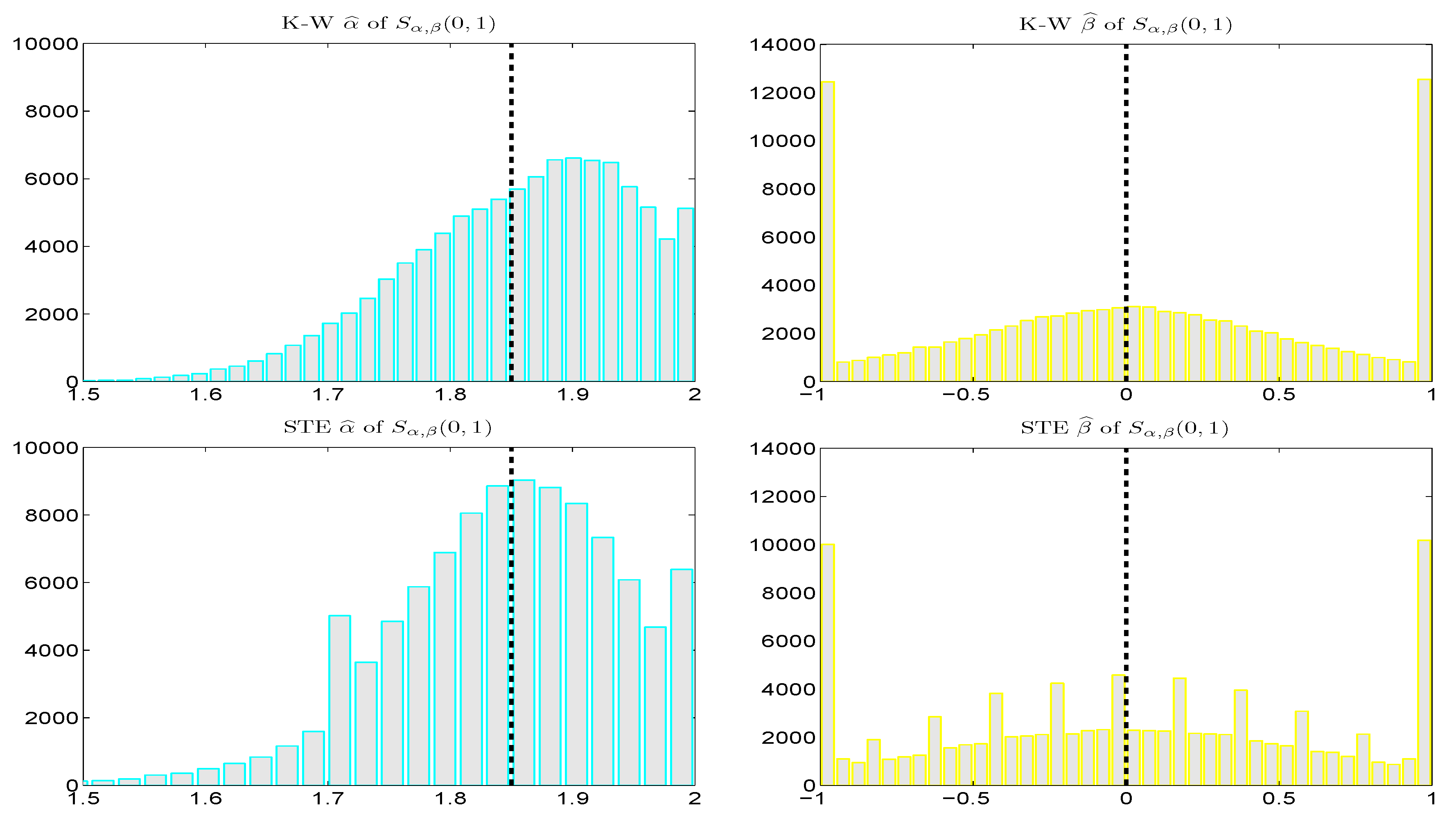
Figure 4 shows the small sample properties of the KW and STE estimators from a simulation study, using true values of α and β that are typical for the conditional innovations process in an $S_{\alpha ,\beta }$-APARCH model, as revealed in Section 7.1 below. For tail index parameter α, we see that the mode of ${\widehat{\alpha }}_{\mathrm{STE}}$ is virtually at the true value, while that of ${\widehat{\alpha }}_{\mathrm{KW}}$ is upward biased. For asymmetry parameter β, ${\widehat{\beta }}_{\mathrm{STE}}$ exhibits less pile-up at the endpoints of the support than does ${\widehat{\beta }}_{\mathrm{KW}}$. The graininess of the former results from the nature of the table lookup. While both methods are vastly faster than use of the MLE, the STE method is about five times faster than KW, thus conveying it yet a further advantage. The empirically computed mean squared error values are, to two significant digits, $\mathrm{MSE}\left({\widehat{\alpha }}_{\mathrm{KW}}\right)=0.0084$, $\mathrm{MSE}\left({\widehat{\alpha }}_{\mathrm{STE}}\right)=0.0087$, $\mathrm{MSE}\left({\widehat{\beta }}_{\mathrm{KW}}\right)=0.40$, and $\mathrm{MSE}\left({\widehat{\beta }}_{\mathrm{STE}}\right)=0.38$.

Thus, in addition to comparable, if not slightly better small-sample performance, the STE method is also much faster. However, as mentioned, its real benefit is its handling of parameter $a_0$ in (14). Much admirable work has been done over the years to enable estimation of the i.i.d. stable model. However, the use of the i.i.d. model in modern, genuine applications is rather limited—once an i.i.d. model is estimated, possibly with an estimator that yields slightly more accuracy in the third significant digit, then what? Our concern is (ultra-) fast estimation of a $S_{\alpha ,\beta }$-APARCH model, given the obvious prominence of GARCH-type effects in financial returns data, with, first, the intent of testing the stability assumption, and secondly, the goal of computing tail risk measures, such as VaR and ES.

As mentioned in Section 3.1, the STE method has been extended to also provide the VaR and ES, based on pre-computation. These otherwise laborious calculations are reduced to essentially instantaneous delivery, and thus can be used for routine calculation by large financial institutions that require reporting the VaR and/or ES on potentially tens of thousands of client portfolios. Moreover, given the near instantaneous calculation of the (parameters, as well as the) VaR and ES for a particular time series under the $S_{\alpha ,\beta }$-APARCH model assumption, the methodology can be used for mean-ES portfolio optimization via the univariate collapsing method; see, e.g., Paolella [45], and thus in the context of risk management. Finally, computation of confidence intervals for these measures are nontrivial and inaccurate using the usual delta-method in conjunction with the sample covariance matrix of the model parameters, rendering the asymptotic distributional behavior of such estimators of little value. Instead, bootstrap methods are required for obtaining accurate confidence intervals of tail risk measures, and thus only consistency (as fulfilled by the STE) is formally required, but practically, also speed, for which the STE method shines.

Remark: 

The method of Kogon and Williams [83] has been extended to the stable-power-GARCH class of models by Francq and Meintanis [100]. They propose an estimation method based on the integrated weighted squared distance between the characteristic function of the stable distribution and an empirical counterpart computed from the GARCH residuals. Under fairly standard conditions, the estimator is shown to be consistent. Future work could consider the efficacy of such an approach compared to the one proposed herein.

6. Simulation Study Under True Model and Variations

First we wish to consider the behavior of the parameter estimates and the p-values of the combined $A+{\tau }_{20}$ test (this being more powerful than either of its two constituent tests) when the simulated model is $S_{\alpha ,\beta }$-APARCH with $a_0=0$, $\alpha =1.85$, $\beta =0$, and APARCH parameters as given in (18). The choice of α is based on the empirical evidence shown in Figure 5, associated with the empirical exercise below in Section 7. 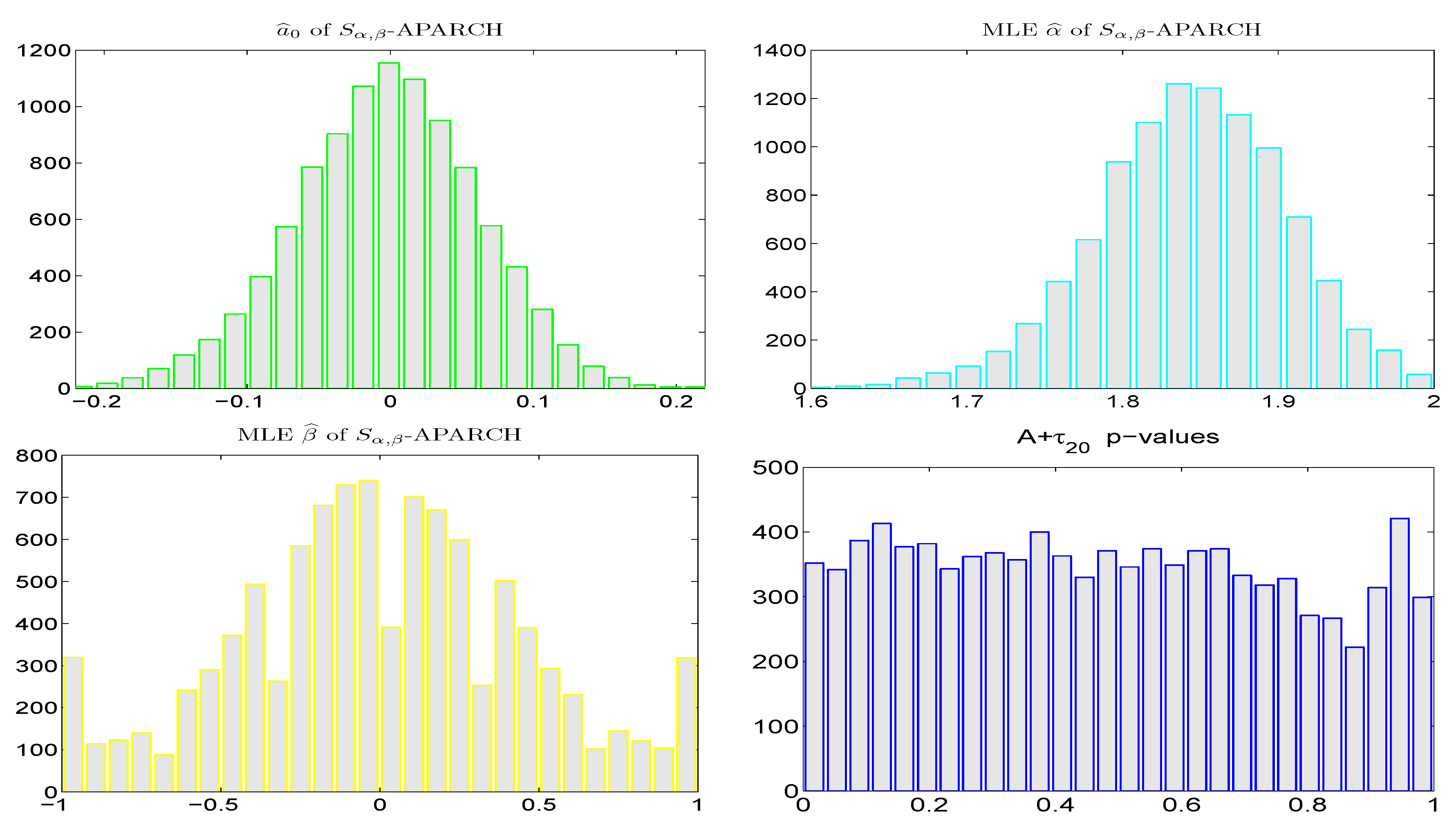Figure 6 shows the results, based on 10,000 replications with sample size $T=500$, using the fixed APARCH parameters (18) and the trimmed mean technique for ${\widehat{a}}_0$ and the fast table lookup method for the two stable shape parameters. Unsurprisingly, given that the true APARCH structure is used, and given the high accuracy of the trimmed mean and table lookup methods, the modes of the histograms of the parameter estimates are at their true values and the shapes of the histograms are very nearly Gaussian (though observe that occasionally, the values of $\widehat{\beta }$ are at the extremes of its parameter space), and the p-values of the $A+{\tau }_{20}$ test are very close to being uniform.

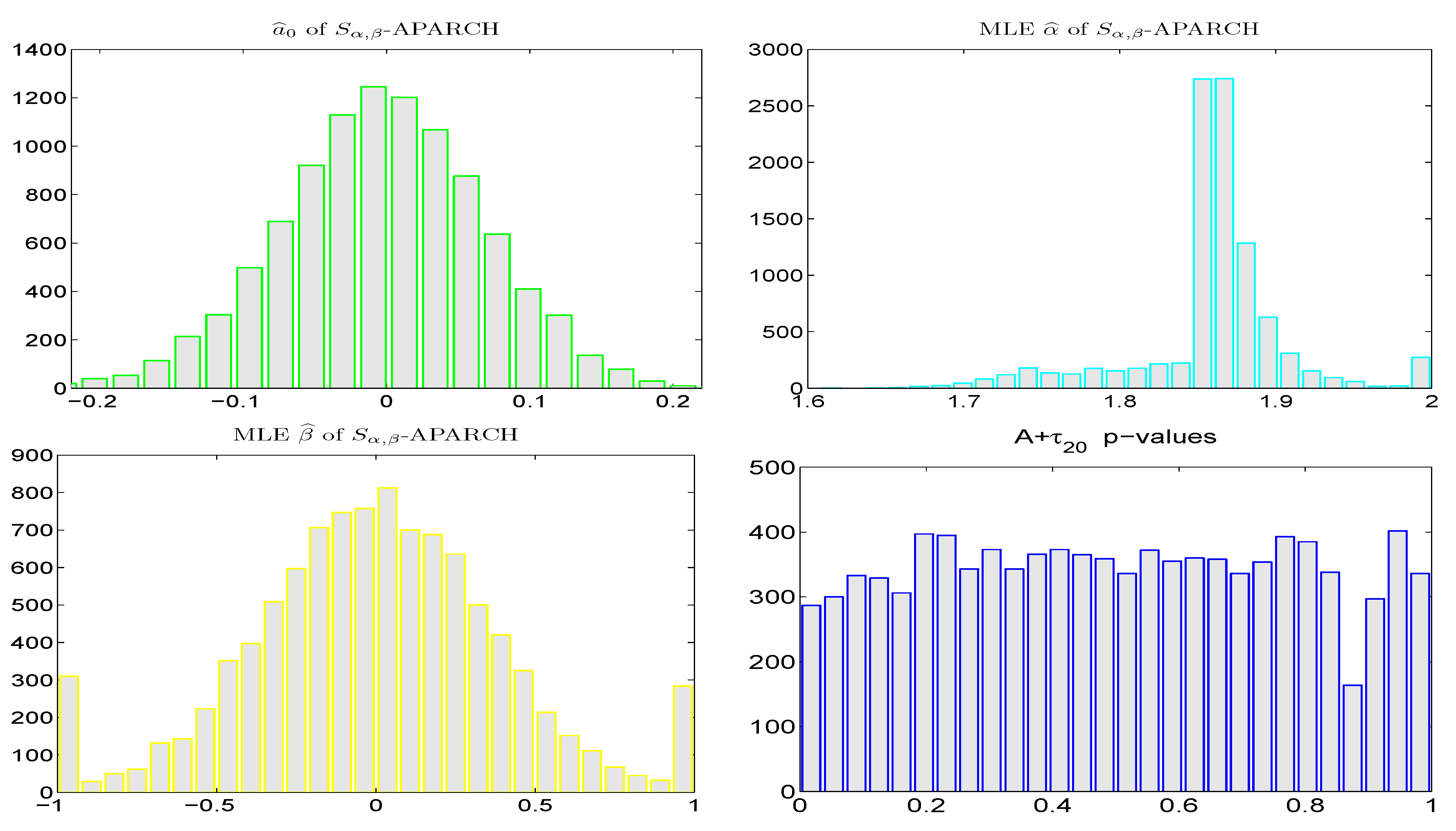
Figure 7 is similar, but having used the jointly computed MLE of all seven model parameters. The results are very similar, including the pileup at the extremes for $\widehat{\beta }$, though for $\widehat{\alpha }$, its empirical distribution is far from Gaussian. To inspect this in more detail, various starting values were used for $\widehat{\alpha }$ (and not just the true value), and the results were always the same. We suspect the reason for this oddly-shaped behavior stems from the use of the fast spline approximation to the stable density used for the MLE calculation. Confirmation could be done using slower but more accurate methods for the calculation of the stable density, but the computing time would then become extensive; and in our context, it is not the primary issue under study.

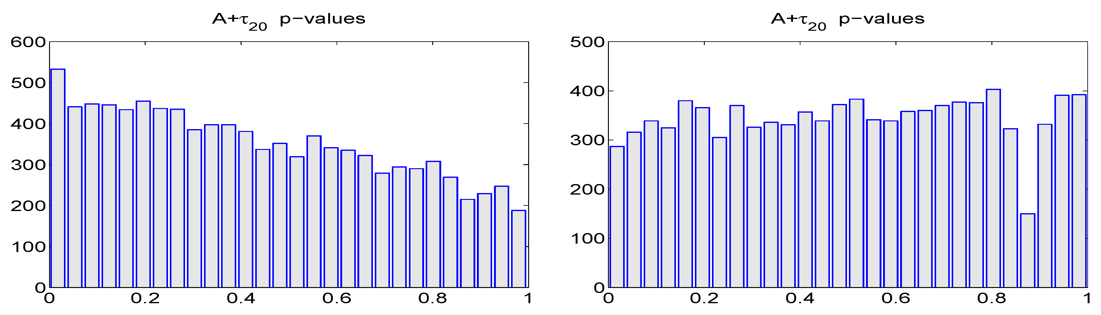
There are obviously infinite ways of modifying the true, simulated data generating process. Figure 8 shows the effect on the p-value of the combined $A+{\tau }_{20}$ test, under the fixed APARCH and MLE settings, when taking $c_1=0.01$ and $d_1=0.95$ (and the remaining parameters as before), this choice being such that the volatility persistence is higher, but the stationarity condition (as a function of $c_1$, $g_1$, α and β, plus $d_1$) is about the same; see Mittnik and Paolella [53] (p. 316) for calculation of the stationarity border in the APARCH case for various distributions. As expected, the p-values of the $A+{\tau }_{20}$ test tend more towards zero when using the fixed, incorrect values of the APARCH parameters (18), while those based on the MLE are still nearly uniform. Further experiments reveal that modifying the true parameter $g_1$ has little effect on the uniformity of the p-values under the fixed APARCH specification (18) (and of course no effect on the MLE-based counterparts), while modifying parameter $c_0$ has a large impact on the former, as well as the parameter estimates of α and β.

7. Empirical Illustration

We apply the above methodology for estimating the $S_{\alpha ,\beta }$-APARCH model to various sequences of asset returns, primarily using the estimation method in (16), given the previous simulation results in Section 6, though we briefly compare the resulting p-values to the use of fixed APARCH parameters in (18).

7.1. Detailed Analysis for Four Stocks from the DJIA Index

We first show the testing results for four daily (log percentage) return series associated with the DJIA index, from 3rd January 2000 to 17 September 2014, using:

• moving windows of length $T=500$ and moving the window ahead by 100 days (resulting in 33 windows of data for each return series);
• moving windows of length $T=1000$ and moving the window ahead by 250 days (resulting in 12 windows of data for each return series);
• the full data set.

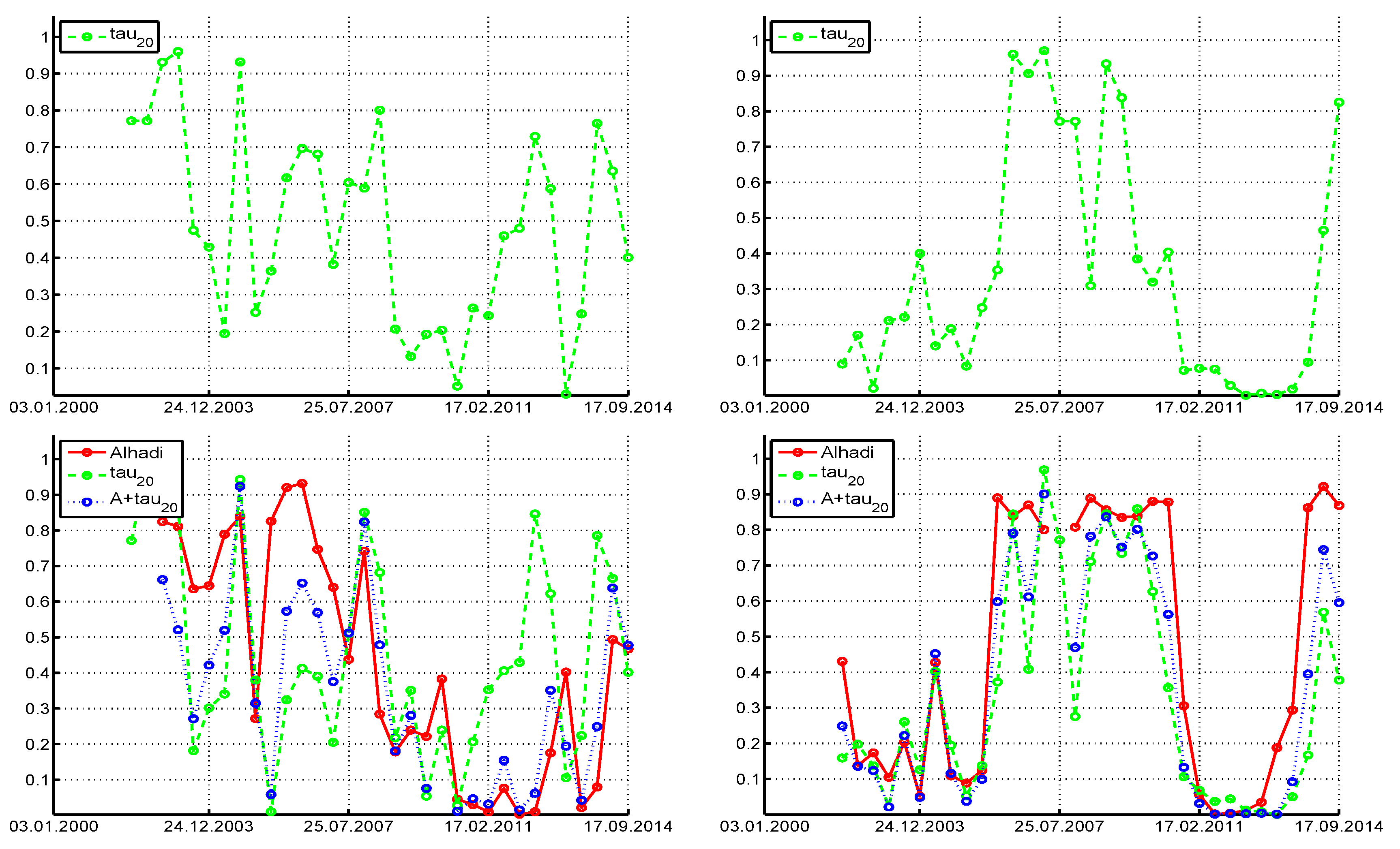
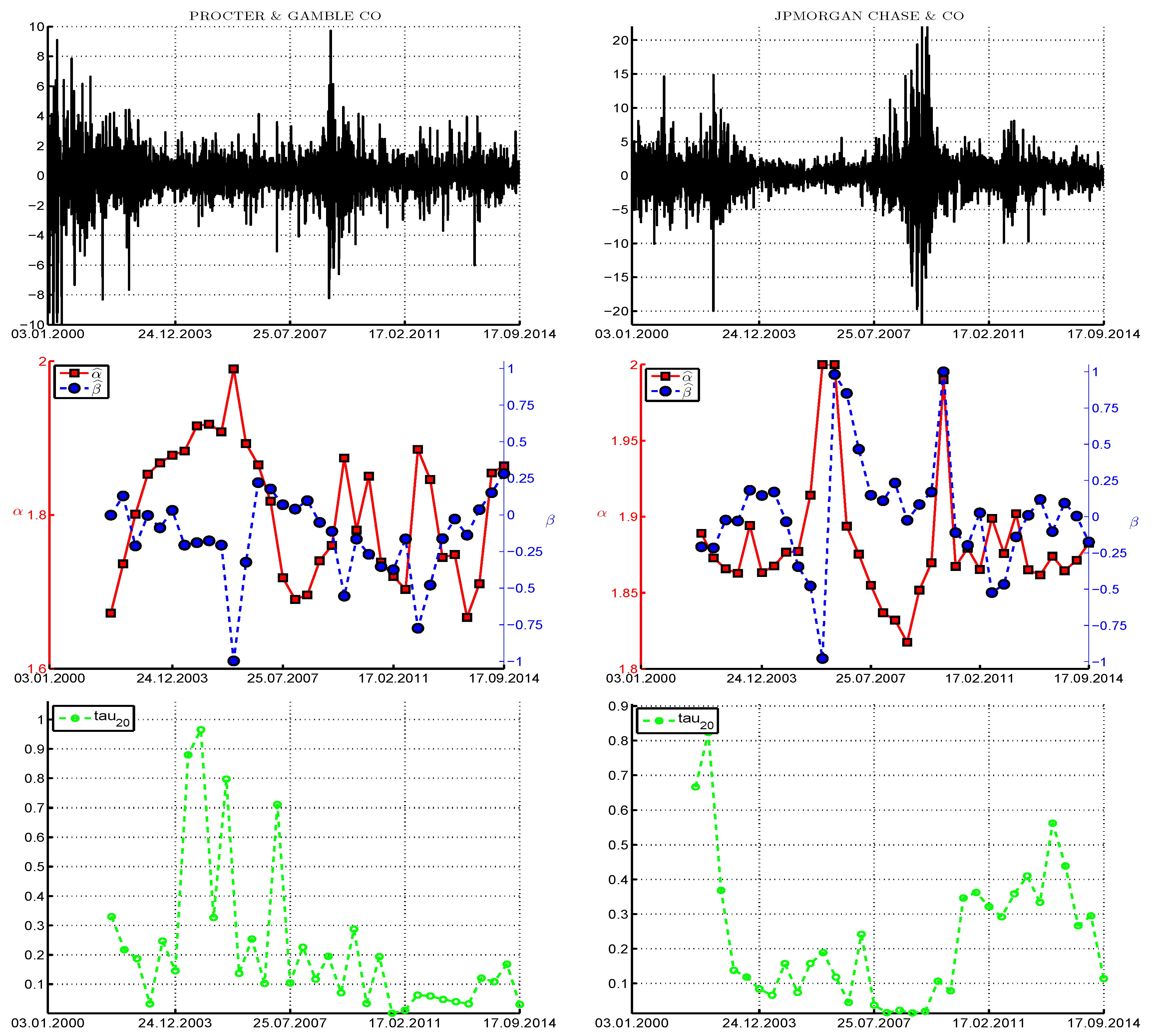
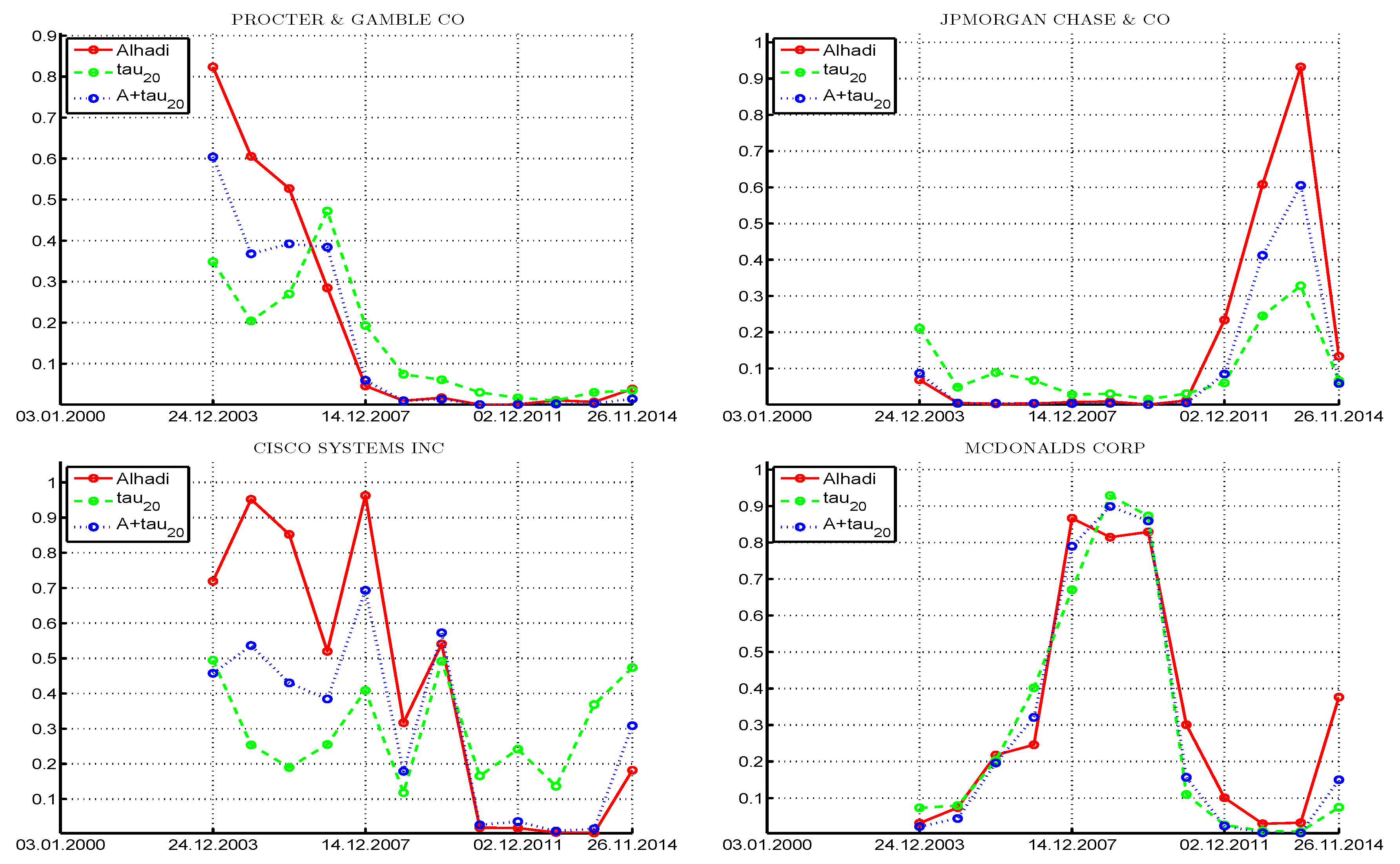
Consider use of the ${\tau }_{20}$ test and ignoring the asymmetry in the returns, recalling that it approximately preserves its size for mildly asymmetric stable Paretian data. To each window, we fit the $S_{\alpha ,0}$-APARCH model as discussed above, and conduct the ${\tau }_{20}$ test on the filtered innovation sequence. The left panels of Figure 9 pertain to the Procter & Gamble company, and show the returns data (top), followed by the estimated values of tail index α (and β, when we consider the tests under asymmetry below), and, in the third panel, the p-values of the ${\tau }_{20}$ test (ignoring asymmetry). (Observe that there is overlap in the data sets used to generate the 33 windows, so that the ${\tau }_{20}$ test p-values are not independent.) Under the null hypothesis (irrespective of the fact that they are not independent) we would expect that their values are uniform on $(0,1)$, and expect one to two of the 33 p-values to lie below 0.05 and about three of them to lie below 0.10. This is clearly not the case, with the vast majority below 0.5, eight values below 0.05, and 13 below 0.10. We conclude, particularly for recent times, that the symmetric stable distribution can be rejected for this model.

Now consider the asymmetric case. The bottom panel shows the p-values from the three tests, ${\tau }_{20}$, ALHADI, and $A+{\tau }_{20}$, based on fitting the $S_{\alpha ,\beta }$-APARCH model and use of the (12) transform. Comparing the ${\tau }_{20}$ results from the symmetric case, we see, as expected, less rejections when asymmetry is accounted for (as the power decreases), but the results are qualitatively the same. The combined test $A+{\tau }_{20}$, which we recall has higher power than its constituent parts, delivers p-values around the region of 2011–2012 very close to zero, providing strong evidence against the stable hypothesis for that time period. With respect to the $\widehat{\alpha }$ and $\widehat{\beta }$ values, observe that, for three windows, $\widehat{\beta }=-1$, but in two of those cases, $\widehat{\alpha }$ is nearly two, in which case, parameter β has no meaning (and is very difficult to estimate). When $\widehat{\alpha }$ is close to two, the ALHADI test does not deliver a statistic, which explains the missing value in the p-value plot.

The right panels of Figure 9 pertain to the JP Morgan Chase company. Similar conclusions hold in the sense that there are periods of data for which the stable hypothesis is clearly rejected, particularly from the combined $A+{\tau }_{20}$ test. It is noteworthy for this data set that, after about 2011, for only one window can the stable hypothesis be rejected.

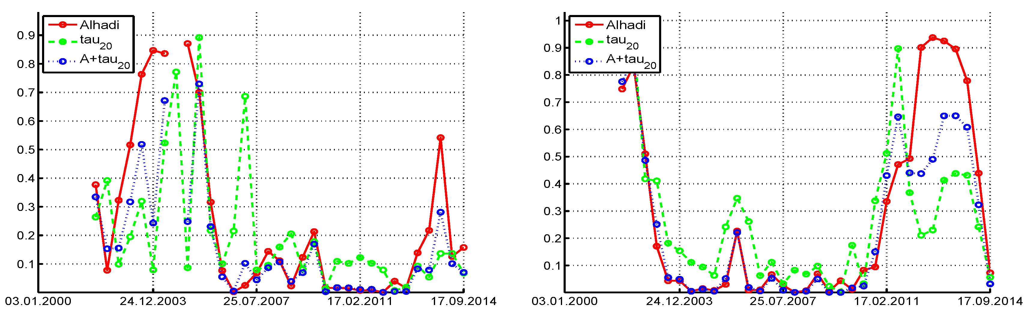
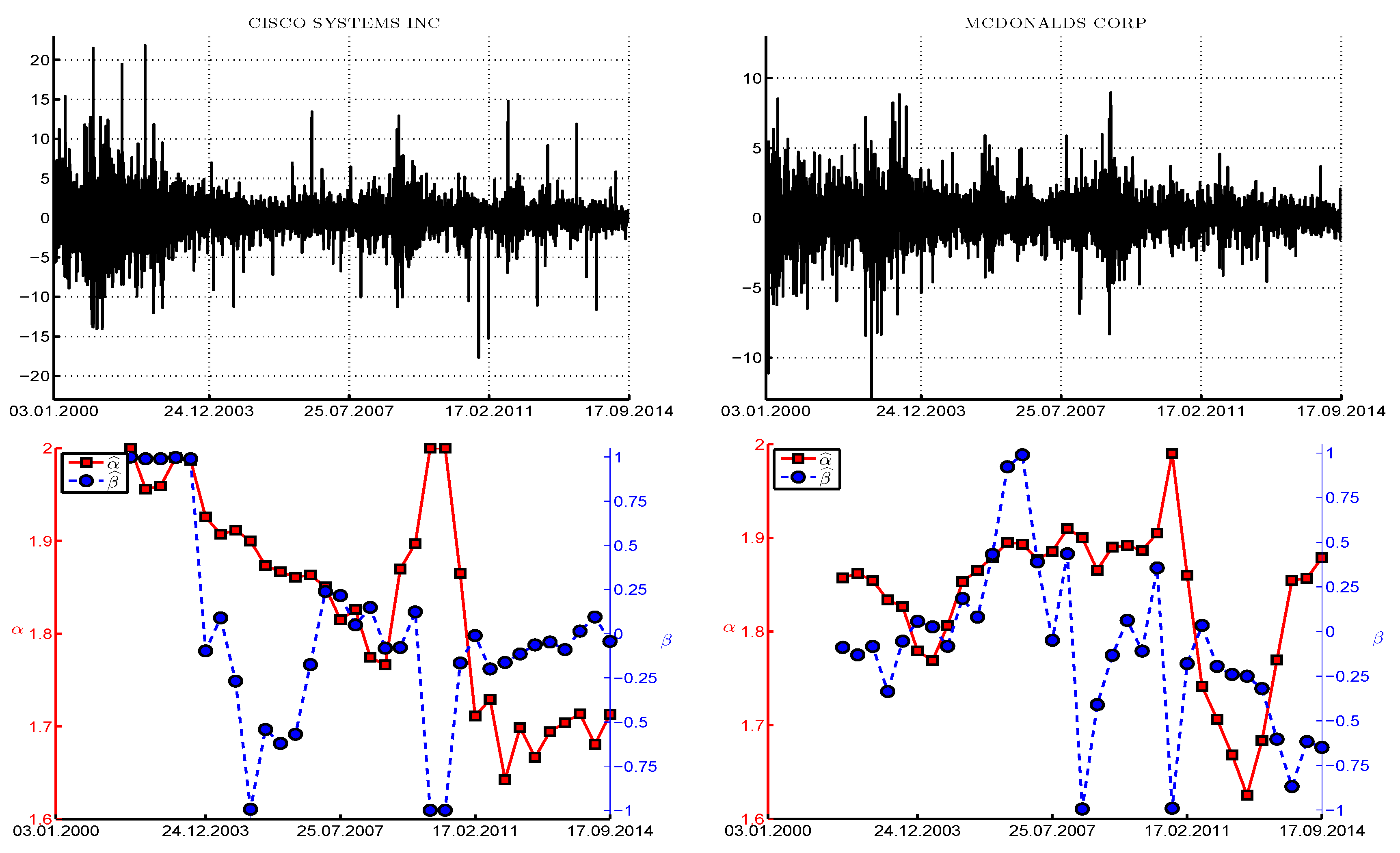
Figure 10 is the same as Figure 9, having used two different stocks, Cisco Systems Inc., and McDonalds Corporation. From the plot of $\widehat{\alpha }$ for Cisco, it appears that, since the year 2003, the risk (as measured by the conditional tail index) increased over much of the time (except for about two years after the high point of the liquidity crisis in 2007), and since about 2011, $\widehat{\alpha }$ is relatively constant around 1.7, and $\widehat{\beta }$ around zero. Use of the ${\tau }_{20}$ test under the assumption of symmetry would suggest that the assumption of stability is tenable for this stock, with rejection at the 10% level only two times out of 33. However, under asymmetry, all three tests reject more frequently with approximately the same proportion. McDonalds yields the interesting observation that, when $\widehat{\alpha }$ decreases, the tests tend to reject the stable assumption.

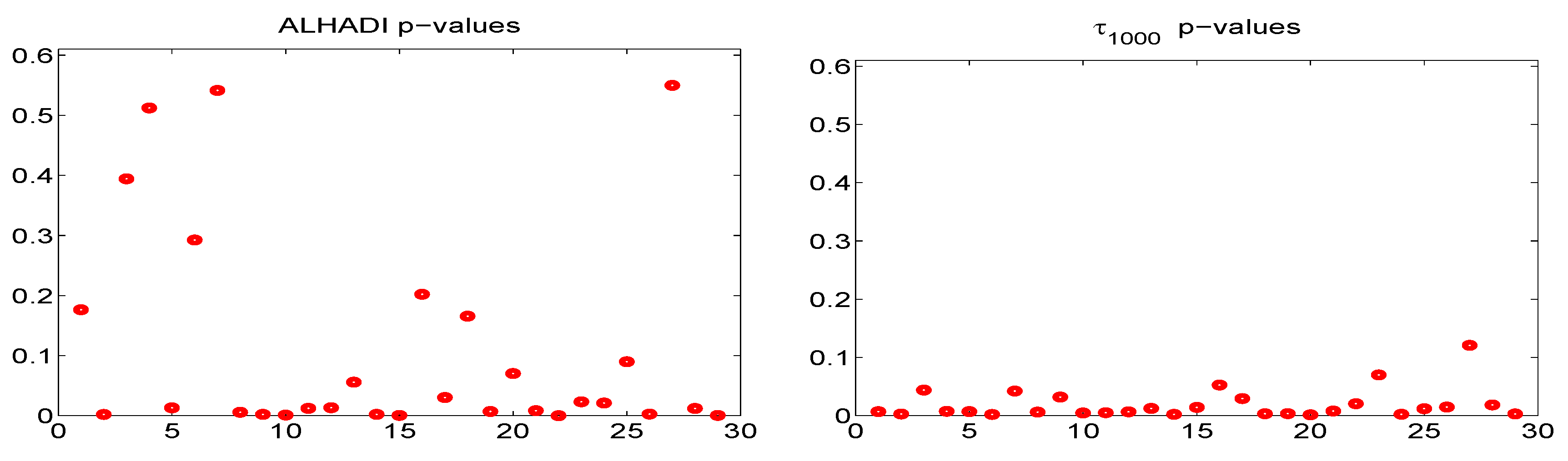
Figure 11 shows the p-values of the three tests when using a window length of $T=1000$ and step size of 250. Qualitatively, they are similar to the $T=500$ case. When using the entire series (with length $T=3773$), the p-values of the ALHADI test are 0.0011, 0.0070, 0.55, and 0.17, for Procter & Gamble, JPMorgan Chase, Cisco Systems, and McDonalds Corp., respectively, while the p-values for ${\tau }_{1000}$ are 0.0041, 0.0043, 0.12, and 0.0034.

Plots associated with the other stocks in the DJIA index were inspected using window lengths $T=500$ and $T=1000$, and reveal similar findings. In particular, there is no stock such that the p-values of the tests appear uniform on $(0,1)$ (with the somewhat exception of Cisco and use of the ${\tau }_{20}$ test under symmetry), but instead, they tend to be closer to zero than one, and tend to have more than two rejections out of 33 at the 5% level and more than three rejections at the 10% level. Given the rejection rates (and the fact that the tests do not have perfect power), it appears that the assumption of stability is not tenable for all stocks and time periods.

7.2. Summary of p-Values from the 29 DJIA Index Stocks

As a summary, and serving as a heuristic for judging the overall assessment of stability in the (APARCH-filtered innovations of the percentage returns of the) stocks, we show the p-values for all stocks and (i) all windows of length $T=500$ and (ii) based on the entire length of the return sequence, as well as looking at the mean rejection rate of the LRT test of size 0.05.

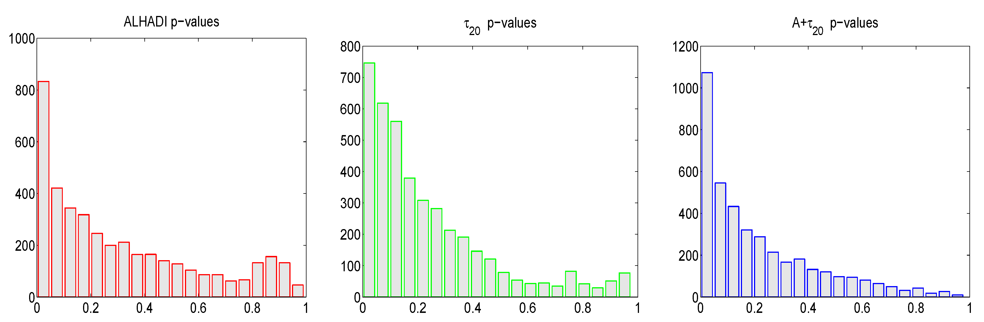
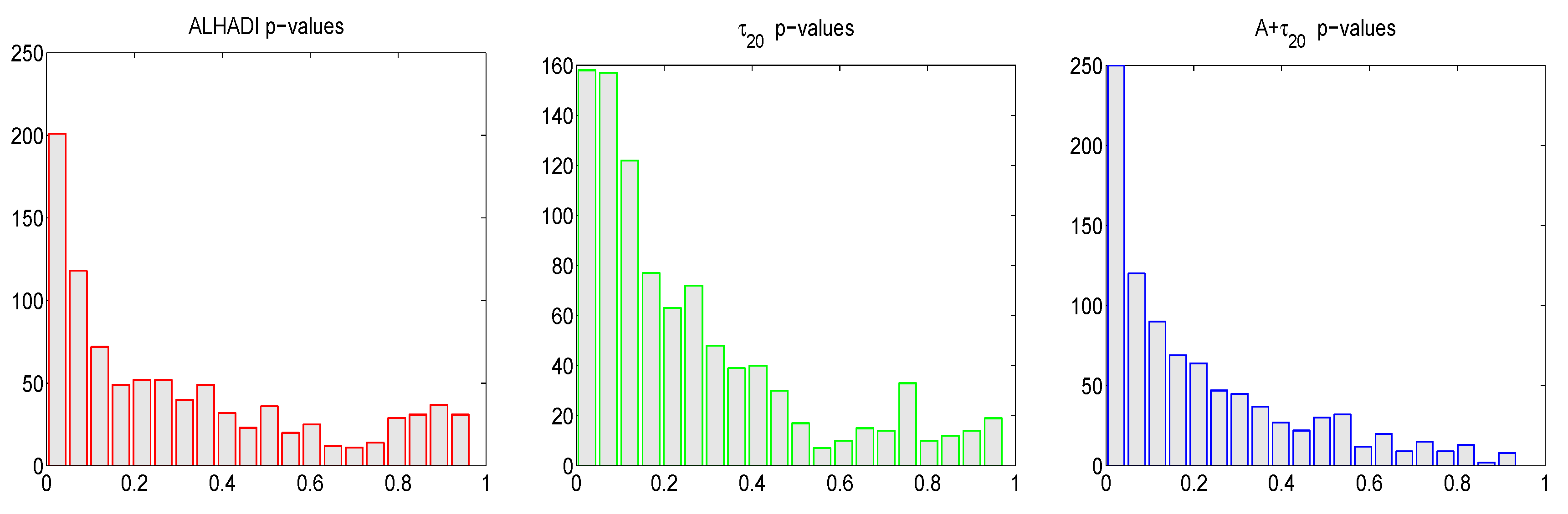
First, Figure 12 shows histograms of the resulting $29\times 33=957$ p-values, for each of the three tests, resulting from use of all 29 available stocks and 33 windows of length $T=500$. (The DJIA Index consists of 30 stocks, but for the dates we use, the Visa company is excluded due to its late IPO in 2008.) As mentioned before, within a stock, the p-values for a particular test are not independent, as the windows overlap. They are perhaps not independent also across stocks. Nevertheless, if the stable hypothesis were true, then the resulting histograms should be close to uniform $(0,1)$. We see that this is not the case, with the deviation from uniformity (and pile-up towards small values) greatest for the $A+{\tau }_{20}$ test, which is precisely the general test with the highest power against numerous alternatives; see Paolella [34]. The mean number of rejections at the nominal level of 0.05 are 0.17, 0.22, 0.28, for the ${\tau }_{20}$, ALHADI, and $A+{\tau }_{20}$ tests, respectively.

When conducting this same analysis using moving windows of length $T=1000$ in increments of 250 (resulting in $29\times 12=348$ time series), the resulting mean number of rejections are 0.27, 0.29, and 0.39. This substantial increase in rejection can be attributed to two factors. The first is that the tests are more powerful as the sample size increases. The second factor is that, unfortunately, as the sample size grows, so does the extent of the misspecification of the model (stable-APARCH, with constant parameters), rendering the filtered innovation sequences less likely to be genuinely i.i.d. Even if (heroically) the $S_{\alpha ,\beta }$-APARCH model assumption were correct at each point in time, then its parameters are changing through time, as observed for the conditional tail index in Figure 9 and Figure 10.

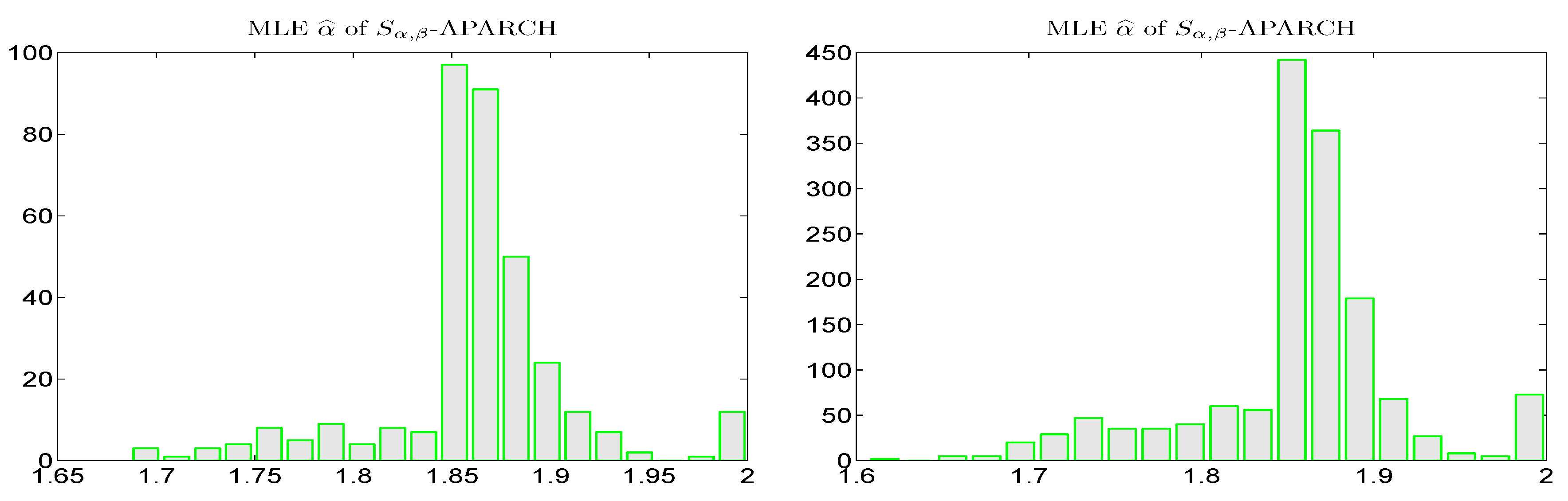
The left panel of Figure 5 shows the estimates of α of the fitted $S_{\alpha ,\beta }$-APARCH process, for the 348 time series of length $T=1000$ from the 29 DJIA stock returns. (The right panel is similar, but applies to the 100 stocks considered in Section 7.3.) We see that, for both data sets, $\widehat{\alpha }$ clusters between 1.85 and 1.9, so that, conditional on the scale term (as modeled via an APARCH process), the conditional distribution of the return is often not particularly heavy-tailed, though still “far” from Gaussian, as can be seen by comparing the, say, 0.01 quantiles or expected shortfall measures of the stable distribution with tail indexes 1.9 and 2.0.

Next, Figure 13 shows the ALHADI and ${\tau }_{20}$ p-values computed on all 29 stocks, using the entire time series of $T=3773$ daily returns, and using $B=1000$ for the ${\tau }_B$ test to ensure near-uniqueness of its values. About 2/3 of the series have ALHADI p-values below 0.10, while 28 of the 29 p-values for the ${\tau }_{1000}$ test are below 0.10, with five close to or above 0.05. This would suggest strong evidence against the stable assumption, but the value of this exercise is somewhat questionable because, as previously mentioned, it assumes that the data generating process is constant throughout the entire time span, and it being a $S_{\alpha ,\beta }$-APARCH process, with constant parameters. For shorter windows, this might indeed be a very reasonable approximation to reality, but for nearly 14 years of daily data, this is highly unlikely, and the resulting sequence of filtered innovations is surely “less close” to being i.i.d. than those corresponding to shorter windows of data.

Finally, we consider the results of the LRT, when applied to the filtered innovation sequence of the fitted $S_{\alpha ,\beta }$-APARCH process applied to the 348 windows of length $T=1000$, this having been estimated by joint maximum likelihood of all seven model parameters, using the spline approximation of the asymmetric stable density provided in Nolan’s toolbox and the method detailed in Krause and Paolella [55] and Paolella [34] for fast estimation of the location-scale NCT. The results of the LRT test are binary, with one indicating rejection at the 5% level. The resulting average rejection rate is 0.47, i.e., for about half of the 348 time series, the stable hypothesis is rejected at the 5% level. This rate is higher than that of $A+{\tau }_{20}$, which was 0.39. One reason is that the LRT is more powerful than $A+{\tau }_{20}$. Another reason is that, possibly, it is also more sensitive to deviations from i.i.d.. Only extensive simulation evidence could shed some partial light on this, but as any GARCH-type model will be misspecified to some extent, particularly as the sample size grows, it is not clear how to definitively address this issue.

Remark: 

Throughout the above analysis, we used the method in (16), such that the APARCH parameters, the location term $a_0$ (based on the trimmed mean method), and two shape parameters of the stable distribution (the latter based on table lookup) are estimated. It is of interest to consider the behavior of the p-values when we fix the APARCH coefficients, as described in (18) (but still estimating $a_0$ and the two stable shape parameters as before). The mean number of rejections at the nominal level of 0.05 are 0.18, 0.19, 0.26, for the ${\tau }_{20}$, ALHADI, and $A+{\tau }_{20}$ tests, respectively. These are very close to the previously obtained numbers but such that the rejection rates for the latter two tests are a bit lower. A possible explanation of this is that the fixed APARCH parametrization is mildly better specified, as argued in Krause and Paolella [55], so that the resulting filtered innovation sequence is “a bit closer to i.i.d.” than its APARCH-fitted counterpart. As the tests assume i.i.d., deviations from this assumption might affect their performance such that the probability of rejection of the null (of i.i.d. stable) is higher when the model is “more misspecified”.

7.3. Summary of p-Values from 100 S&P500 Stocks

Here we consider a larger data set, using the daily percentage log returns from the top 100 market-cap corporations of the S&P500 index (obtained from CRSP), from 3rd January 1997 until 31st December 2014. The results are shown in Figure 14, which is similar to Figure 12, but based on the resulting 4100 p-values, from the 100 stocks and 41 windows of length $T=500$ incremented by 100 days. We observe a similar phenomenon as with the DJIA stocks, namely, that the p-values for all the tests are not uniform on $(0,1)$, but rather indicative that the stable assumption can be rejected for some stocks and time periods. The mean number of rejections at the nominal level of 0.05 are 0.19, 0.21, 0.27, for the ${\tau }_{20}$, ALHADI, and $A+{\tau }_{20}$ tests, respectively. Again notice that the latter has the highest rejection rate, as it is the most powerful of the three tests.

When conducting this same analysis using moving windows of length $T=1000$ in increments of 250 (resulting in 1500 time series), the resulting mean number of rejections are 0.36, 0.32, and 0.48. The LRT test, applied to the same windows, yields an average rejection rate of 0.50, i.e., for half of the 1500 time series, the stable assumption is rejected at the 5% level. Observe that the rejection rate using the LRT is the highest among all the tests considered, while that of the combined $A+{\tau }_{20}$ was very close, being 0.48.

8. Conclusions

A fast new method for estimating the parameters of the $S_{\alpha ,\beta }$-APARCH is developed, and this is used to obtain the filtered innovation sequences when the model is applied to daily financial asset returns data. These are, in turn, subject to several new tests for stability. Application of the tests to the components of the DJIA-30 index and the top 100 market-cap corporations of the S&P500 index suggests that, for most stocks and some segments of time, the assumption of the innovation process driving a GARCH-type process being i.i.d. stable Paretian cannot be rejected, though overall, based on the rejection rates, there is evidence against it.

One should differentiate in this context between the use of formal testing procedures for a distributional assumption, and the appropriateness, or lack thereof, of using that distribution. In particular, the successful use of the stable distribution in conjunction with GARCH-type models for risk prediction and asset allocation lends evidence that, at least from a purely practical point of view, the model has merit. This point is also made in Nolan [101]. Moreover, a very large number of empirical studies exist that use a GARCH model with Student’s t or generalized exponential (GED) innovations, these being available in many software packages, but rarely, if ever, is the distributional assumption questioned or addressed in a formal way. Instead, some studies will compare the forecasting performance of several models, usually finding that the use of a GARCH-type model that allows for asymmetric shocks to volatility, in conjunction with a leptokurtic, asymmetric distribution, delivers competitive risk forecasts.

All models and distributions employed for modeling non-trivial real data are nothing but approximations and are necessarily wrong; and without an infinite amount of data, tail measurements will always be inaccurate. As such, at least in finance, while distributional testing is an important diagnostic, a crucial measure of the utility of a model is in the application to forecasting, such as downside risk, or portfolio optimization—for which different (non-Gaussian) models can be compared and ranked.

Both in-sample and out-of-sample diagnostics and testing procedures have value for assessing the appropriateness of a model, but the purpose of the model must always be considered. For example, if tomorrow’s VaR is required on 100,000 portfolios, then speed, numeric reliability, and practicality will play a prominent role. In the complicated game of financial risk forecasting and asset allocation, it is highly unlikely that a single model will be found to consistently outperform all others, but the appropriate use of distributional testing, out-of-sample performance diagnostics, and common sense can lead to a model that reliably fulfils its purpose.