Volatility Forecasting: Downside Risk, Jumps and Leverage Effect

Abstract

We provide empirical evidence of volatility forecasting in relation to asymmetries present in the dynamics of both return and volatility processes. Using recently-developed methodologies to detect jumps from high frequency price data, we estimate the size of positive and negative jumps and propose a methodology to estimate the size of jumps in the quadratic variation. The leverage effect is separated into continuous and discontinuous effects, and past volatility is separated into “good” and “bad”, as well as into continuous and discontinuous risks. Using a long history of the S & P500 price index, we find that the continuous leverage effect lasts about one week, while the discontinuous leverage effect disappears after one day. “Good” and “bad” continuous risks both characterize the volatility persistence, while “bad” jump risk is much more informative than “good” jump risk in forecasting future volatility. The volatility forecasting model proposed is able to capture many empirical stylized facts while still remaining parsimonious in terms of the number of parameters to be estimated.

1. Introduction

Volatility forecasting is crucial for many investment decisions, such as asset allocation and risk management. This paper presents empirical results on volatility forecasting of a stochastic process with asymmetries and discontinuities in the return and volatility processes, highlighting the importance of incorporating these effects into the forecasting model itself. Moreover, a methodology for separating realized volatility into quarter variances and for estimating volatility jumps is introduced.

Asymmetries, discontinuities and memory properties in the data-generating process for asset returns are known stylized facts. Specifically, these are also known as the volatility leverage and feedback effects that induce skewness, infrequent jumps that induce fat tails and volatility persistence representing the process memory. The existence of these effects poses challenges for obtaining accurate volatility forecasts and requires models that can take into account all of those empirical features. Capturing volatility persistence, the popular heterogeneous autoregressive realized volatility model ($HAR-RV$) of [1], which is based on an approximation of long-run volatility components, performs surprisingly well in out-of-sample forecast evaluations.

The realized volatility, advocated by, among others, [2] and [3], consistently estimates the integrated volatility of the return process under the assumption that it follows a continuous semimartingale. Realized volatility is based on the notion of increasing sampling frequency and is generally considered an accurate proxy for the latent true volatility. These kinds of non-parametric estimates are particularly suited for forecasting, as jump information can be extracted directly from the data, and volatility persistence, leverage and feedback effects can be modeled parsimoniously in the framework of a simple regression.

Evidence of the leverage effect with high frequency data has been advanced by Bollerslev, T. et al. [4], who analyzed sign asymmetries of high frequency returns and their impact on future volatility. This paper presents new evidence of leverage effects by using high frequency data of the S & P500 Index. To the prior literature, it adds the consideration of a separate leverage effect generated by both the jump and the continuous components of the return process.

The main empirical contribution of this paper is the finding of a superior forecasting performance when the jumps in returns are isolated from the corresponding continuous component. While the previous papers separated jump variation and continuous variation, as proposed by Andersen, T.G. et al. [5], here, we disentangle the jump size from the continuous return at the intraday level and include it in the prediction model. With this approach, on top of improving forecasting performance, we could also interpret any effect of return jumps on future volatility as a jump leverage effect. As in [1], we include in the forecasting model the long memory of volatility considering heterogeneous autoregressive ($HAR$) components and, as in [6], the continuous leverage effect through lagged negative returns generated from continuous components.

Further, as in [7], we find that the best forecasting model includes “downside risks,” which are volatilities generated by negative intraday returns. The realized variance is in fact also disentangled into continuous signed semi-variations and jump signed semi-variations, as a way to capture separate dynamics of negative intraday returns with respect to positive intraday returns. The leverage effect in forecasting realized volatility has been considered by both Corsi, F. and Renò, R. [6] and Patton, A.J. and Sheppard, K. [7] in a similar framework. These papers are the most closely related to our study. However, the methodology to assess it differs as we disentangle jump size from both return and volatility, and we also separate both jump variation and continuous variation into semi-variances. Particularly relevant for our analysis of return jumps and asymmetries between jump components is the methodology to detect intraday return jumps proposed by Lee, S.S. and Mykland, P.A. [8].

Methodologically, using the return jump detection methodology of [8], we derive a complete decomposition of the realized variance into four quarter variances, two signed jump variations and two signed continuous variations. To our knowledge, a complete linear decomposition of the realized variance into quarter variances is new in the literature. The work in [9] proposed the decomposition of the realized variance into semi-variances, while Patton, A.J. and Sheppard, K. [7] proposed a different method of estimating signed jump semi-variances, but together with the continuous variation, they do not sum to the total realized variance. Moreover, we propose a jump identification method for the quadratic variation based on auxiliary inference. As the return may jump, the quadratic variation may also jump if the underlying data-generating process is a double jump stochastic process. These are the two methodological contributions of this paper.

The literature on jump detection and realized volatility forecasting has become very rich in the last 10 years. Focusing on return jumps, Dumitru, A.M. and Urga, G. [10] performed an extensive Monte Carlo study of the performance of nine methods to detect jumps. They find that the methodology used in this paper based on [8] performs better than the alternatives and is more robust to microstructure noise. 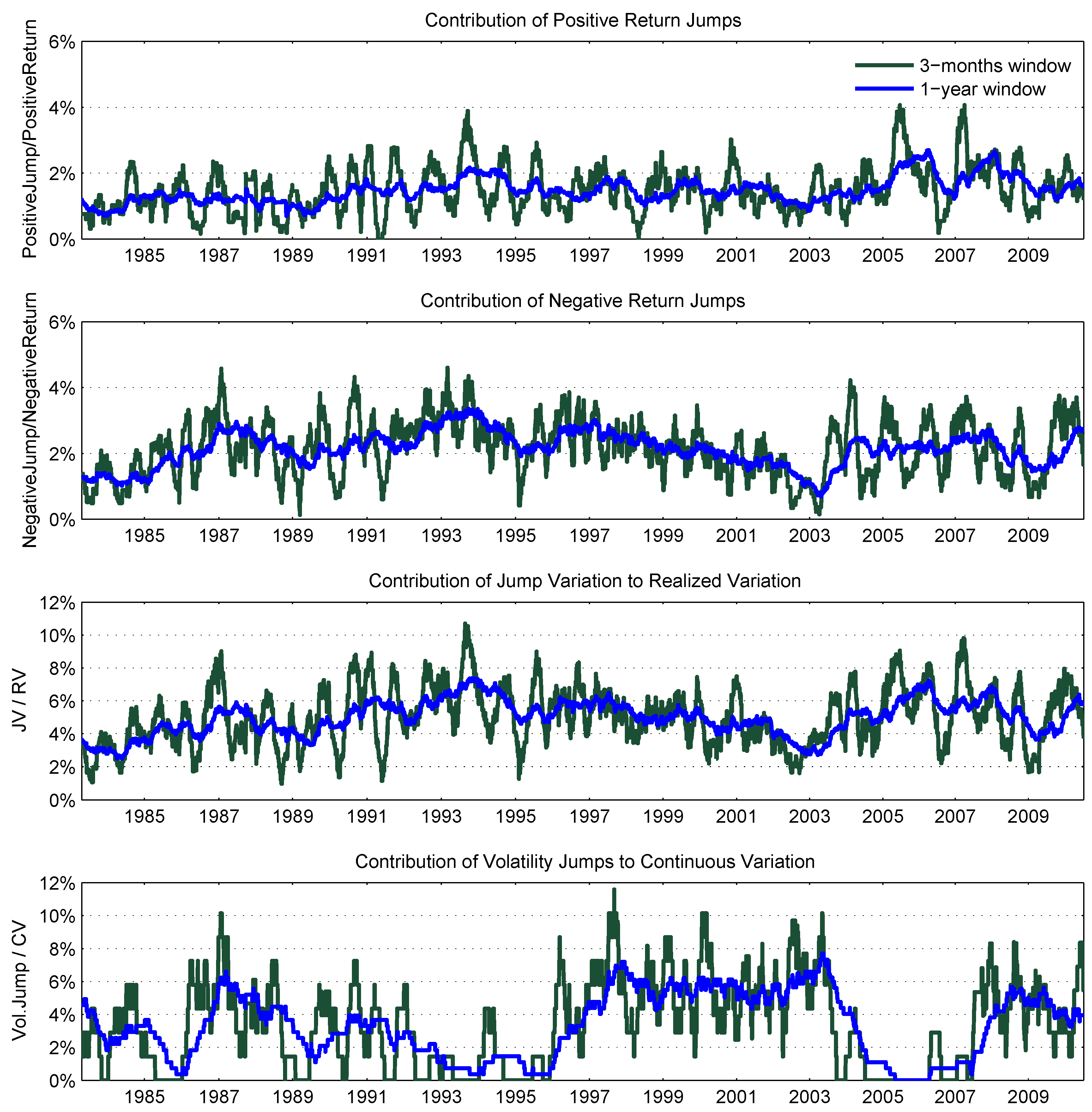In this paper, we ignore microstructure noise and do not compare the performance of jump detection procedures, but rather, we compare the performance of volatility forecasting models that are based on the chosen jump detection methodology introduced in [8].1

Using a different jump test, Huang, X. and Tauchen, G. [12] studied the power of their jump detection test statistics and presented evidence of daily jump frequency in the S & P500 financial market. They found that for the S & P500 Index futures, the contribution of jump variation to total variation is between 4.4% and 4.6% for the time period from 1997 to 2003. The work in [13] used ultra-high frequency data (tick-by-tick) to study the contribution of jump variation to total variation for a large set of securities. Their jump variation is estimated as the difference between total variation and continuous variation, with the two components, in turn, estimated by pre-averaged returns in a local neighborhood to be robust to noise and outliers. They found that jump variation estimated with ultra-high frequency data is of an order of magnitude lower than jump variation estimated with five minute price data. In this paper, we sample at five minutes to smooth microstructure noise, and unlike the previous paper, using a high-frequency jump test, we are able to estimate jump variation directly from the return jump size instead of resorting to the daily difference of estimated total and continuous variation. With this method of estimating jump variation, we find the contribution of jump variation to be in line with [12]2. As pointed out in [13], with a higher sampling frequency, the jump variation magnitude may be different, and the estimates of jump variation based on five minute data may capture variation in liquidity. We do not aim to justify jumps and study microstructure noise effects, but rather, compare the out-of-sample forecasting performance of an imperfect proxy, such as the realized volatility.

Using daily price data, Jacquier, E. and Okou, C. [14] separated jump from continuous variation to predict future excess returns. Their paper is related to the intertemporal capital asset pricing literature. They found evidence of past continuous variation having a longer lasting effect in pricing than jump variation. While focusing on volatility forecasting, we find that continuous variation is the driving factor for the persistence in volatility. In contrast, the effect of jumps is short-lived. This is in line with the finding of [14].

The remainder of the paper is organized as follows. Section 2 presents realized estimators used in the analysis, the continuous time framework on which the estimates are based and the methodology to disentangle continuous and jump components from both return and volatility processes. Section 3 presents the data used in the empirical analysis and the candidate forecasting models. Section 4 contains evidence of the leverage and jump effects and presents estimation results and the out-of-sample forecasting performance evaluation. Finally, Section 5 concludes.

2. Theoretical Framework

The underlying framework for the empirical analysis is based on a double jump-diffusion data-generating process. This stochastic process features a continuous sample path component and occasional jumps in both return and volatility dynamics. The framework was first laid down by Duffie, D. et al. [15]. The empirical analysis of this class of models can be found in [16,17,18,19,20]. Generally, the previous results support jumps in volatility, as well as jumps in returns for speculative prices. Let $s_t$ denote the logarithmic asset price at time t, for $t\in [0,T]$. In stochastic differential equation form, the price and volatility processes are

$$\begin{array}{ccc}\hfill d{s}_t& =& m_{t}dt+{\sigma }_{t}d{W}_t^s+{\kappa }_t^{s}d{J}_t^s,\hfill \end{array}$$

(1)

$$\begin{array}{ccc}\hfill d{\sigma }_t^2& =& \vartheta \left(\theta -{\sigma }_t^2\right)dt+{\sigma }_t^{v}d{W}_t^v+{\kappa }_t^{v}d{J}_t^v,\hfill \end{array}$$

(2)

where $\left\{W_t^s,W_t^v\right\}$ is a bivariate standard Brownian motion, $\left\{d{J}_t^s,d{J}_t^v\right\}$ is a bivariate count process and $\left\{{\kappa }_t^s,{\kappa }_t^v\right\}$ represents the size of the jumps in return and in volatility if a count occurs at time t3. The mean of the variance Equation (2) is characterized by a long-run level parameter θ and a mean-reverting parameter ϑ. Moreover, the process is restricted to be non-negative.

This framework allows the generation of the contemporaneous leverage or volatility feedback effects through the correlation between the continuous components, as well as through the correlation between the jump components that may be both in the time and in the size of the jumps.

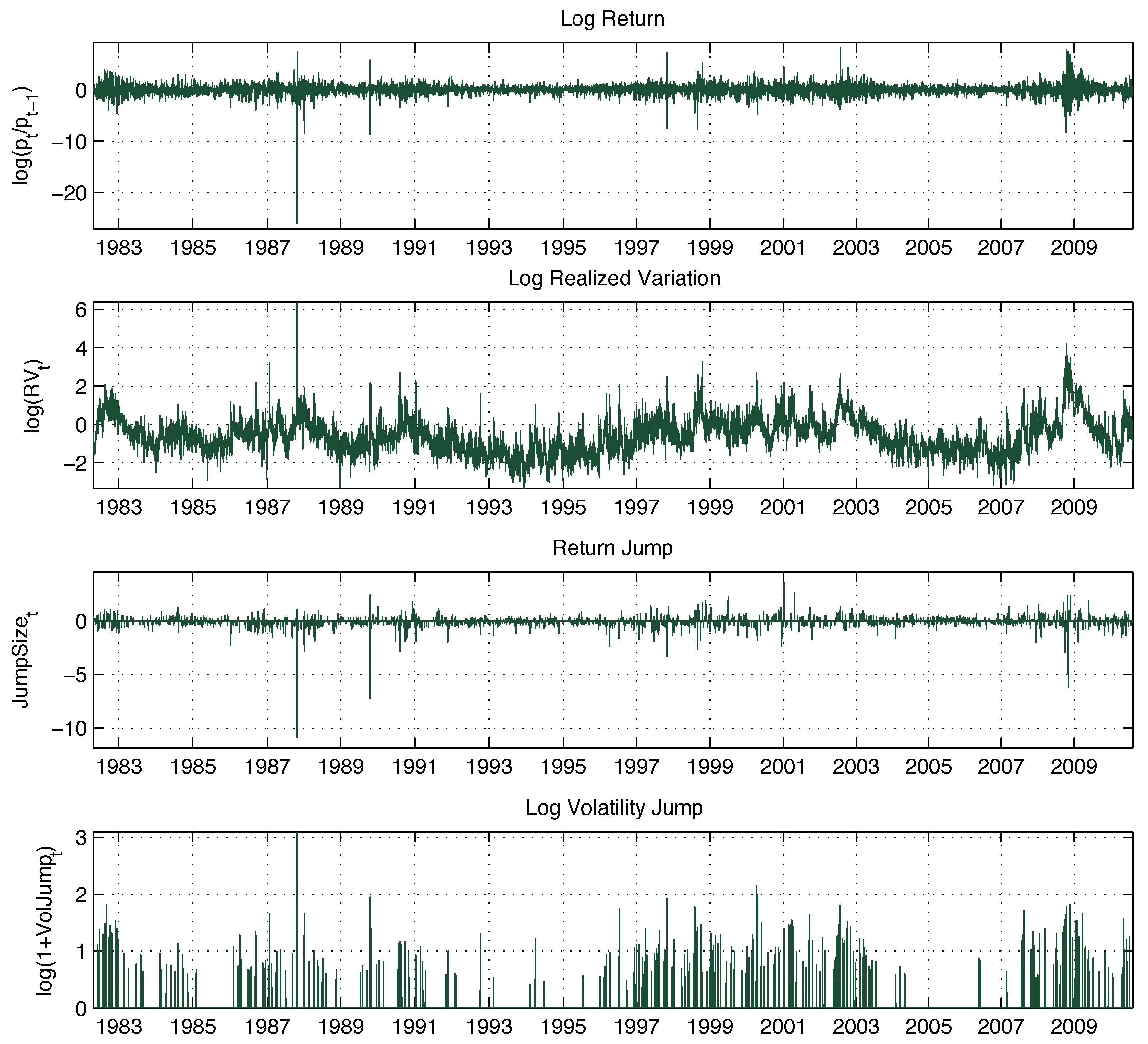
Following the theory of quadratic variation, the volatility of the price process is estimated with the realized volatility from high frequency data. Below, we present the estimators for volatility and jump components used in the analysis.

2.1. Return Volatility and Jumps

Let $r_{t,i}$ be the discretely-sampled i-th intraday return for day t. In the presence of jumps in return, the realized variance, $R{V}_t={\sum }_{i=1}^m{r}_{t,i}^2$, introduced by Andersen, T.G. et al. [2] and Andersen, T.G. et al. [21], captures both continuous and jump components of the quadratic variation:

$$R{V}_t\stackrel{p}{⟶}{\int }_{t-1}^t{\sigma }_{\tau }^{2}d\tau +\sum _{t-1<\tau \le t}{\left({\kappa }_{\tau }^s\right)}^{2}t=1,\dots ,T.$$

(3)

The bi-power variation, introduced by [22], is instead a consistent estimator for the continuous component only:

$$B{V}_t={\mu }^{-2}\sum _{i=2}^m\left|r_{t,i}\right|\left|r_{t,i-1}\right|\stackrel{m\to \infty }{⟶}{\int }_{t-1}^t{\sigma }_{\tau }^{2}d\tau$$

(4)

where $\mu =2^{1/2}\frac{\Gamma \left(1\right)}{\Gamma \left(1/2\right)}$=$\sqrt{2/\pi }$, with $\Gamma \left(·\right)$ denoting the gamma function.

The work in [23] and [8] proposes detecting intraday jumps using the ratio between intraday returns and estimated spot volatility. We follow more closely the methodology of [8], and in particular, we test the presence of intraday jumps with the statistics

$${\mathcal{L}}_{t,i}=\frac{r_{t,i}}{\sqrt{\left(\frac{1}{K-1}{\sum }_{k=1}^{K-1}\left|r_{t,i-k}\right|\left|r_{t,i-k-1}\right|\right)}},$$

(5)

where the expression contains in the denominator the estimates of the spot volatility as the average bi-power variation over a period with K observations. Lee, S.S. et al. [8] suggests using $K=78,110,156,270$, respectively, with return sampled at frequencies of 60, 30, 15 and 5 minutes. Under the null of no intraday jump, the test statistics ${\mathcal{L}}_{t,i}$ follow a normal distribution (with variance $\sqrt{2/\pi }$).

In order to select the rejection region for the test statistics ${\mathcal{L}}_{t,i}$, Lee, S.S. et al. [8] propose to look at the asymptotic distribution of maxima of the test statistics. As the sampling frequency tends to zero, under the null of no jumps between time $\left(t,i-1\right)$ and $\left(t,i\right)$, the absolute value of ${\mathcal{L}}_{t,i}$ converges to a Gumbel distribution:

$$\frac{{max}_{\left(t,i\right)}\left|{\mathcal{L}}_{t,i}\right|-C_n}{S_n}\stackrel{d}{⟶}\zeta ,$$

(6)

where ζ has a standard Gumbel distribution, $C_n=\frac{{\left(2logn\right)}^{1/2}}{\mu }-\frac{log\pi +log\left(logn\right)}{2\mu {\left(2logn\right)}^{1/2}}$, $S_n=\frac{1}{\mu {\left(2logn\right)}^{1/2}}$ and n is the number of observations for each period t. We reject the null of no jump at time $t,i$ if

$$\frac{\left|{\mathcal{L}}_{t,i}\right|-C_n}{S_n}>{\beta }^{*},$$

(7)

such that $exp\left(-e^{-{\beta }^{*}}\right)=1-\alpha$, i.e., ${\beta }^{*}=-log\left(-log\left(1-\alpha \right)\right)$, with α being the significance level4.

The test is able to detect the jump arrival time $i_j$ for each day t, where j denotes the presence of a jump. Moreover, the jump size is computed as

$${\kappa }_{t,i_j}=\left(r_{t,i}\right){\mathbb{1}}_{\left\{\frac{\left|{\mathcal{L}}_{t,i}\right|-C_n}{S_n}>{\beta }^{*}\right\}}.$$

(8)

consequently, the jump size for the day t is

$$jRe{t}_t=\sum _{i_j=i_1,\dots ,i_{J_t}}{\kappa }_{t,i_j},t=1,\dots ,T,$$

(9)

where $J_t$ is the total number of significant jumps for day t, and the jump-adjusted daily return is

$$cRe{t}_t=r_t-jRe{t}_t,t=1,\dots ,T.$$

(10)

With this methodology to identify intraday jumps, it is possible to directly estimate the jump variation, i.e., the quadratic variation of return jumps. We follow [25] and estimate the quadratic variation due to the continuous and the jump components respectively as

$$\begin{array}{ccc}\hfill C{V}_t& =& R{V}_t-J{V}_t,t=1,\dots ,T,\hfill \end{array}$$

(11)

$$\begin{array}{ccc}\hfill J{V}_t& =& \sum _{j=1}^{J_t}J{V}_{t,j},t=1,\dots ,T,\hfill \end{array}$$

(12)

where

$$J{V}_{t,j}={\mathbb{1}}_{\left\{{\kappa }_{t,i}\ne 0\right\}}\left({\kappa }_{t,i_j}^2-\frac{1}{m-J_t}\sum _{k\in \left\{1,\dots m\right\}\backslash \left\{i_j,\dots ,i_{J_t}\right\}}{r}_{t,k}^2\right),$$

(13)

is the contribution to the quadratic variation of each intraday jump ${\kappa }_{t,i_j}$, with $j=1,\dots ,J_t$ and $t=1,\dots ,T$. We find that the daily jump variation identified with this methodology is highly correlated with more traditional methods to identify jump variation that primarily take the positive differences between $R{V}_t$ and $B{V}_t$.

2.2. Downside Continuous and Jump Variation

To capture the sign asymmetry of the volatility process, the continuous variation and jump variation are decomposed using signed intraday returns. The work in [9] introduced a new estimator that captures the quadratic variation due to signed returns, termed realized semi-variance. In a similar way, the continuous variation and jumps variation can both be decomposed into signed semi-variations by using the test of [8]. This represents the main advantage of the test, as it is able to identify the sign and the timing of intraday jumps. If jump variation is instead identified by means of significant $\left(R{V}_t-B{V}_t\right)$, as normally done in the previous literature, no information is available about the sign or timing of intraday jumps, and therefore, we are not able to disentangle jump or continuous semi-variations.

The realized semi-variances of [9] are defined as

$$\begin{array}{ccc}\hfill R{S}_t^{+}& =& \sum _{i=1}^m{r}_{t,i}^2{\mathbb{1}}_{\left\{r_{t,i}>0\right\}},\hfill \end{array}$$

(14)

$$\begin{array}{ccc}\hfill R{S}_t^{-}& =& \sum _{i=1}^m{r}_{t,i}^2{\mathbb{1}}_{\left\{r_{t,i}<0\right\}}.\hfill \end{array}$$

(15)

We estimate the jump semi-variances in a similar fashion by using signed intraday jumps:

$$\begin{array}{ccc}\hfill JS{V}_t^{+}& =& \sum _{j=1}^{J_t}JS{V}_{t,j}^{+},\hfill \end{array}$$

(16)

$$\begin{array}{ccc}\hfill JS{V}_t^{-}& =& \sum _{j=1}^{J_t}JS{V}_{t,j}^{-},\hfill \end{array}$$

(17)

where

$$\begin{array}{ccc}\hfill JS{V}_{t,j}^{+}& =& {\mathbb{1}}_{\left\{{\kappa }_{t,i}>0\right\}}\left({\kappa }_{t,i_j}^2-\frac{1}{m-J_t}\sum _{k\in \left\{1,\dots m\right\}\backslash \left\{i_j,\dots ,i_{jt}\right\}}{r}_{t,k}^2\right),\hfill \end{array}$$

(18)

$$\begin{array}{ccc}\hfill JS{V}_{t,j}^{-}& =& {\mathbb{1}}_{\left\{{\kappa }_{t,i}<0\right\}}\left({\kappa }_{t,i_j}^2-\frac{1}{m-J_t}\sum _{k\in \left\{1,\dots m\right\}\backslash \left\{i_j,\dots ,i_{jt}\right\}}{r}_{t,k}^2\right),\hfill \end{array}$$

(19)

for $j=1,\dots ,J_t$ and $t=1,\dots ,T.$ Consequently, the continuous semi-variances are estimated by

$$\begin{array}{ccc}\hfill CS{V}_t^{+}& =& R{S}_t^{+}-JS{V}_t^{+},\hfill \end{array}$$

(20)

$$\begin{array}{ccc}\hfill CS{V}_t^{-}& =& R{S}_t^{-}-JS{V}_t^{-}.\hfill \end{array}$$

(21)

The realized variance is decomposed into quarter variances, and this decomposition is complete as $R{V}_t=R{S}_t^{+}+R{S}_t^{-}$, $J{V}_t=JS{V}_t^{+}+JS{V}_t^{-}$ and $C{V}_t=CS{V}_t^{+}+CS{V}_t^{-}$. To study the volatility feedback effect, a particular focus is on the downside continuous variation and jump variation captured by $CS{V}^{-}$ and $JS{V}^{-}$, respectively, as Patton, A.J. and Sheppard, K. [7] show that negative semi-variances are more informative than positive semi-variances for forecasting future volatility. These quantities are used in the empirical analysis of the following sections.

2.3. Volatility Jumps

The estimation of volatility jumps is a prominent topic of research (see [20]). The difficulty in estimating volatility jumps is due to the model misspecification of the jump process coupled with the fact that volatility is a latent quantity. Here, we consider a methodology to estimate the size of (continuous) volatility jumps without imposing assumptions on its distribution while we assume that the realized variance estimate (continuous variation given in Equation (11)) is the true variance, as is standard practice in the realized variance literature.

We consider an auxiliary first order autoregressive $\left(AR\left(1\right)\right)$ model on the first difference of continuous variation with the variance of continuous variation following generalized autoregressive conditional heteroskedasticity $\left(GARCH\left(1,1\right)\right)$ dynamics. This choice is motivated empirically and theoretically. The $AR-GARCH$ on the changes in continuous volatility is a natural discrete approximation of the volatility process in Equation (2) without the volatility jump component, with the $AR\left(1\right)$ approximating the volatility mean and the $GARCH\left(1,1\right)$ equation capturing the volatility of volatility. Empirically, it fits very well with the continuous variation sample series by excluding extreme values. It is specified as

$$\begin{array}{ccc}\hfill {\left(\Delta CV\right)}_t& =& c+\varphi C{V}_{t-1}+u_t,\hfill \end{array}$$

(22)

$$\begin{array}{ccc}\hfill u_t& =& {\sigma }_t^v{e}_t,e_t\sim N\left(0,1\right),\hfill \end{array}$$

(23)

$$\begin{array}{ccc}\hfill {\left({\sigma }_t^v\right)}^2& =& \omega +\alpha u_{t-1}^2+\beta {\left({\sigma }_{t-1}^v\right)}^2,\hfill \end{array}$$

(24)

with stationarity constraint $\left|\varphi \right|<1$, $\left(\alpha +\beta \right)<1$ and non-negativity constraints on ${\left({\sigma }_t^v\right)}^2$: $\omega >0,\left\{\alpha ,\beta \right\}\ge 0$. The jump in volatility is estimated as

$$Vol{J}_t={\mathbb{1}}_{\left\{e_t>{\Phi }_{1-\alpha }^{-1}\right\}}{u}_t,$$

(25)

where ${\Phi }_{1-\alpha }^{-1}$ denotes the $1-\alpha$ quantile of the standard normal distribution, and the indicator for the timing of volatility jumps is given by $e_t>{\Phi }_{1-\alpha }^{-1}$.5 Intuitively, in the absence of volatility jumps, the auxiliary model approximates the true volatility dynamics. However, in the presence of large jumps, the auxiliary model is not able to fit the data, and large residuals from the model fit represent contributions of volatility jumps.

At this point, it is worth reiterating that the estimated volatility jumps are in fact jumps of the continuous variation, where the continuous variation is an estimate of the variance process without return jumps. Given the double-jump process as the data-generating process, the continuous variation may well jump itself, even without jumps in the return process. The combination of the terms “jumps in continuous variation” may sound paradoxical. Therefore, the term “volatility jumps” instead of “jumps in continuous variation” is used.

3. Data and Forecasting Models

3.1. Data and Summary Statistics

The data used in the analysis consist of tick-by-tick prices for the Standard & Poor (S & P500) Future. The sample period covers almost the entire history of this security: from 28 April 1982 to 6 August 2010. The S & P500 Future is traded “open outcry” on regular market opening hours of the Chicago Mercantile Exchange (from 8:30 a.m. to 3:15 p.m.), and it has also been used by Bollerslev, T. et al. [26] and Corsi, F. [1], among others, as an index for the composite market.

The data cleaning procedure follows [27]. In particular, as trades before 9:00 a.m. for the first several years from the introduction of this security are often not very active, all trades outside 9:00 a.m. and 3:15 p.m. are discarded. Transactions with zero volume are also discarded. Moreover, days with less than five consecutive trading hours are also discarded. Prices are then sampled every five minutes, starting from 9:00 a.m., in order to smooth the impact of market microstructure noise. Furthermore, whenever there is no observed price attached to a specific time stamp, the “previous tick” method is used to replace the missing price.

Figure 1 represents the time series of returns, log realized variance, return jumps and volatility jumps. The highest levels of realized volatility were reached on “Black Monday,” 19 October 1987, and the following day, 20 October, where returns were respectively about −26% and −9.6%. The test Equation (7) detects jumps during both days. However, for 19 October 1987, the intraday price changes were less drastic than on the following day, resulting in a lower jump variation. On 20 October 1987, jump variation was at the highest level. During that day, negative jumps were combined with positive jumps, while on 19 October, sequences of negative intraday returns dominated. The jumps test are carried out through the analysis with an $\alpha =0.01$ significance level.

Jumps in volatility are also identified for both 19 and 20 October 1987, with the volatility jump for 19 October being at the highest level. Accordingly, the market crash of 19 October 1987 is explained with jumps in returns and even more with a jump in volatility. This underscores the importance of allowing for volatility jumps in order to fully capture the dynamics of extreme events. Return jumps alone, identified with the testing methodology, are not able to fully account for extreme market events. Summary statistics for the intensity of jumps in return and in volatility are reported in

Table 1. The table reports the number of days with return jumps, their percentage, the average daily jump intensity conditional on the presence of at least one jump, the maximum daily jump intensity and the percentage of days with jumps in continuous variation. All of the statistics are sorted by year. The tests for jumps in return and in continuous variation are conducted with significance level $\alpha =0.01$. * The sample period for 1982 starts on 20 April; $**$ The sample period for 2010 stops on 6 August.

Year	n. Days with Return Jump	% Days with Return Jump	Mean Jump Intensity (One Day)	Max Jump Intensity (One Day)	% Days with Volatility Jump
1982*	31	17.92	1.10	3	6.94
1983	29	11.51	1.38	6	1.98
1984	48	19.05	1.13	2	3.57
1985	50	19.76	1.22	4	0.40
1986	48	18.97	1.60	7	5.14
1987	36	14.63	1.89	10	5.28
1988	45	17.86	1.47	6	3.97
1989	42	16.67	1.48	8	2.38
1990	47	18.65	1.51	5	3.17
1991	48	19.05	1.46	8	2.78
1992	60	23.9	1.47	8	1.20
1993	67	26.59	1.51	6	0.40
1994	57	22.71	1.47	5	1.59
1995	48	19.2	1.38	4	0.40
1996	49	19.6	1.49	5	4.40
1997	48	19.35	1.77	6	7.26
1998	48	19.2	1.33	4	5.20
1999	49	19.6	1.39	4	5.60
2000	39	15.6	1.59	7	6.00
2001	39	15.92	1.41	3	5.71
2002	33	13.31	1.12	3	7.66
2003	50	20.16	1.12	3	4.03
2004	47	19.34	1.43	4	1.23
2005	67	27.13	1.33	4	0.00
2006	50	20.24	1.32	4	0.81
2007	60	24.19	1.65	7	3.63
2008	48	19.43	1.38	4	7.29
2009	44	17.6	1.41	5	4.80
2010**	35	23.33	1.49	4	4.67
Full Sample		19.29	1.43		3.65

.

On average, there is less than one return jump per day. With significance level $\alpha =0.01$ and five minute sampling, the number of days with at least one intraday jump represents 19.29% of the sample period. The intraday jump intensity ranges from zero to 10 jumps (maximum corresponding to 19 October 1987). Conditional on the presence of jumps, there are on average 1.43 intraday return jumps each day. Regarding jumps in volatility, we find an intensity of about 6.65% of the trading days. The analysis for volatility jumps is also carried out at significance level $\alpha =0.01$ in Equation (25). As with jumps in return, other significance levels are experimented with. The chosen cutoff level $\alpha =0.01$ is empirically motivated by the quantile-quantile plot shown in Figure 2.

The empirical distribution with this cutoff level best approximates a standard normal distribution. Without a threshold, the residuals from the auxiliary $GARCH$ model fitting deviate substantially from the assumed standard normal distribution. Only large departures from the standard normal distribution are categorized as volatility jumps.

The contribution of return jumps to total return levels, the relative contribution of jump variation to the total variation and the contribution of volatility jumps to the continuous volatility are reported in Figure 3.

The contribution of negative jumps to negative returns appears to be higher, on average, than the contribution of positive jumps to the corresponding signed returns. This jump sign asymmetry may account for the negative skewness observed in financial markets. Based on rolling averages of three-month and one-year windows, the contribution of the negative jumps to corresponding signed returns ranges from approximately 0.1% to 4.5%, on a three-month basis, and from 1% to 3.5%, on a yearly basis, while that of positive jumps ranges from 1% to 2.5%, on a yearly basis. Jump variation accounts for approximately 3% to 7% on a yearly basis. This statistic is in line with those reported by the previous literature despite the use of a different methodology to test for the presence of jumps. The work in [6], for example, reports an average percentage over almost 28 years of about 6% for the S & P500 Index; Andersen, T.G. et al. [25] report an average percentage over five years that ranges from 2.1% to 5.8% for different stocks; and Huang, X. and Tauchen, G. [12] report an average of 4.4% to 4.6% between 1997 and 2003 for the S & P500 Index. By contrast, volatility jumps make a minor contribution to the continuous variation, as they are more sporadic than return jumps. They account for about 0% to 8% of the continuous variation on a yearly basis, and for the entire sample period from 1982 to 2010, they represent 3.4% of continuous variation.

3.2. Forecasting with Jumps, Leverage Effect and Volatility Persistence

Given the measures of volatility and jump magnitude introduced previously, it is of interest to study their additional forecasting power for future volatility. The models proposed are based on the heterogeneous autoregressive ($HAR$) framework of [1] and extend it by considering semi-variances, jumps in return and in volatility and the leverage effect due to continuous return and return jumps.

The realized volatility features long memory. The $HAR$ model, although it does not belong formally to the class of long memory models, represents a parsimonious approximation, which is able to closely mimic such a stylized fact. In more detail, the benchmark model is

$$log{\left(RV\right)}_{t,t+h}=\alpha +{\varphi }^{d}log{\left(RV\right)}_t+{\varphi }^{w}log{\left(RV\right)}_{t-5,t}+{\varphi }^{m}log{\left(RV\right)}_{t-22,t}+erro{r}_t,$$

(26)

where $log{\left(RV\right)}_{t,t+h}$ is the average log realized variance between time t and $t+h$. The variables $log{\left(RV\right)}_{t-5,t}=\frac{1}{5}{\sum }_{i=t-4}^{t}log\left(R{V}_i\right)$ and $log{\left(RV\right)}_{t-22,t}=\frac{1}{22}{\sum }_{i=t-21}^{t}log\left(R{V}_i\right)$ capture long memory features of the volatility process. The coefficients of the model may be interpreted as the reaction of heterogeneous agents who forecast with different time horizons: daily, weekly and monthly. The representation of the $HAR$ forecasting model based on realized variance instead of log realized variance,

$${RV}_{t,t+h}=\alpha +{\varphi }^{d}R{V}_t+{\varphi }^{w}R{V}_{t-5,t}+{\varphi }^{m}R{V}_{t-22,t}+erro{r}_t,$$

(27)

is also considered. However, the latter produces inferior forecasts, and therefore, results are summarized and discussed for the log-log model.

Several model extensions based on the $HAR$ framework have been proposed in the recent literature: see, among others, [5,6,7]. The work in [5] included jump variation in forecasting volatility dynamics. The work in [6] studied the impact of the leverage effect on volatility by including past signed returns. Finally, Patton, A.J. and Sheppard, K. [7] and Chen, X. and Ghysels, E. [28] considered the use of realized semi-variances to forecast volatility. None of the previous studies, however, used the return jumps themselves and jumps in volatility to generalize the $HAR$ model.

Jumps in return arguably have an impact on future volatility. Their effect can be interpreted as a leverage effect. The leverage effect can manifest itself differently if it comes about through continuous jump returns. In fact, although both continuous and discontinuous components together generate the final leverage effect, their dynamics differ, as jumps have a very short impact on future volatility, while continuous returns tend to have a persistent impact on future volatility.

Disentangling jump variation and continuous variation systematically improves volatility forecasts, and disentangling downside semi-variation and upside semi-variation also improves forecasts. We combine the ideas of [5] and [7] by considering a complete decomposition into signed continuous and jump variation, leading to even better forecasts. Negative jump semi-variation has in fact a completely different impact on future volatility compared to positive jump semi-variation. Lastly, jumps in volatility may also improve future volatility forecasts through the effect of volatility trading strategies. Taking into account all of these effects, the candidate model we propose is

$$\begin{array}{ccc}\hfill log{\left(RV\right)}_{t,t+h}& =& \alpha +{\beta }^{+}log{\left(CS{V}^{+}\right)}_t+{\beta }^{-}log{\left(CS{V}^{-}\right)}_t\hfill \\ & +& {\gamma }^{+}log{\left(1+JS{V}^{+}\right)}_t+{\gamma }^{-}log{\left(1+JS{V}^{-}\right)}_t\hfill \\ & +& \theta log{\left(1+VolJ\right)}_t+\delta cRe{t}_t^{-}+{\delta }_{w}cRe{t}_{t-5,t}^{-}\hfill \\ \mathrm{(28)}& & +& {\vartheta }_{w}log{\left(RV\right)}_{t-5,t}+{\vartheta }_{m}log{\left(RV\right)}_{t-22,t}+erro{r}_t,\hfill \end{array}$$

where past negative returns and jumps are defined by $cRe{t}_t^{-}={\mathbb{1}}_{\left\{cRe{t}_t<0\right\}}cRe{t}_t$ and $cRe{t}_{t-5,t}^{-}=\frac{1}{5}{\sum }_{i=t-4}^{t}cRe{t}_i^{-}$. Note that the realized jump semi-variances already capture the effect of return jumps, since they are derived from them. The interpretation of their effects is that of discontinuous risks that capture jump leverage effects. Therefore, return jumps are not included in this model specification.

Given that one of the goals of this study is volatility forecasting, one can argue that such a model may be over-parametrized and therefore may lead to poor out-of-sample results. As we will show in the next sections, this is not (entirely) the case. Nevertheless, to overcome this problem, we consider a simplified version of Model (28) that differs from the previous one by discarding jump semi-variations, the weekly persistence in the leverage effect and the jumps in volatility6. Moreover, the impact of jump semi-variations on future volatility is being replaced by that of return jumps, which is to be interpreted as a leverage effect due to jumps:

$$\begin{array}{ccc}\hfill log{\left(RV\right)}_{t,t+h}& =& \alpha +{\beta }^{+}log{\left(CS{V}^{+}\right)}_t+{\beta }^{-}log{\left(CS{V}^{-}\right)}_t+\delta cRe{t}_t^{-}\hfill \\ & +& \phi jRe{t}_t+{\vartheta }_{w}log{\left(RV\right)}_{t-5,t}+{\vartheta }_{m}log{\left(RV\right)}_{t-22,t}+erro{r}_t.\hfill \end{array}$$

(29)

this model is very simple, consisting of only seven parameters to be estimated, e.g., three parameters less than the $LHAR-CJ$ model proposed by Corsi, F. et al. [6]. Still, the model focuses on the most relevant effects for volatility forecasting: downside risk, leverage effect and the $HAR$ structure capturing long memory.

The models are estimated by $OLS$ with [29] covariance matrix correction to account for serial correlation. The bandwidth used is $2\left(h-1\right)$, where h is the forecasting horizon.

4. Empirical Evidence

4.1. Leverage Effect, Volatility Feedback Effect and Persistence

Leverage and volatility feedback effects are commonly studied by means of correlations. The work in [4] provides exhaustive evidence of the leverage effect at high frequency by studying cross-correlations among return and volatility series for a horizon spanning several days. Exploiting the methodology we use to disentangle the continuous and jump components of return and volatility dynamics, we present new evidence of leverage and volatility feedback effects arising from both continuous and jump components. Moreover, we use signed intraday returns to capture sign asymmetries.

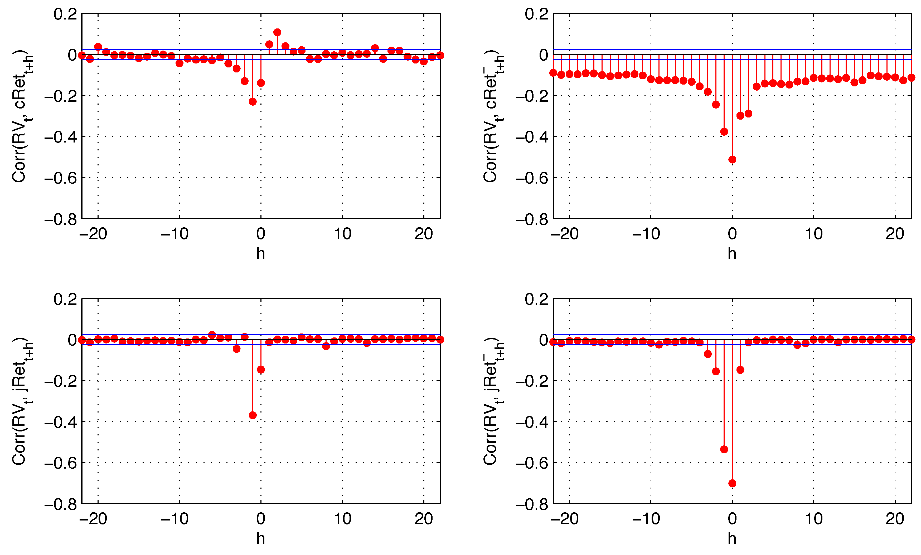
Figure 4 reports cross-correlations among different components of the return and realized variance as evidence of leverage and volatility feedback effects.

As in [4], the leverage effect (negative correlation between $R{V}_t$ and $cRe{t}_{t-h}$) is significant for prolonged days, while there is no clear evidence of a volatility feedback effect (negative correlation between $R{V}_t$ and $cRe{t}_{t+h}$). The sign asymmetry of the leverage effect becomes evident as negative returns generate most of the negative correlation of return and lagged variance (see top right plot, Figure 4), and the magnitude of this effect is higher than the positive correlation between positive returns and realized variance. We also observe a negative correlation between realized variance and future negative returns. However, this correlation is smaller in absolute value than the positive correlation of realized variance and positive future returns (cross-correlations with positive intraday return components are not plotted in order to save space). Therefore, it is insufficient to generate the sign asymmetry for the volatility feedback effect. In other words, while negative returns have a higher impact on future variance than positive returns (leverage effect), the variance does not have a higher impact on future negative returns than it does on future positive returns (no volatility feedback effect).

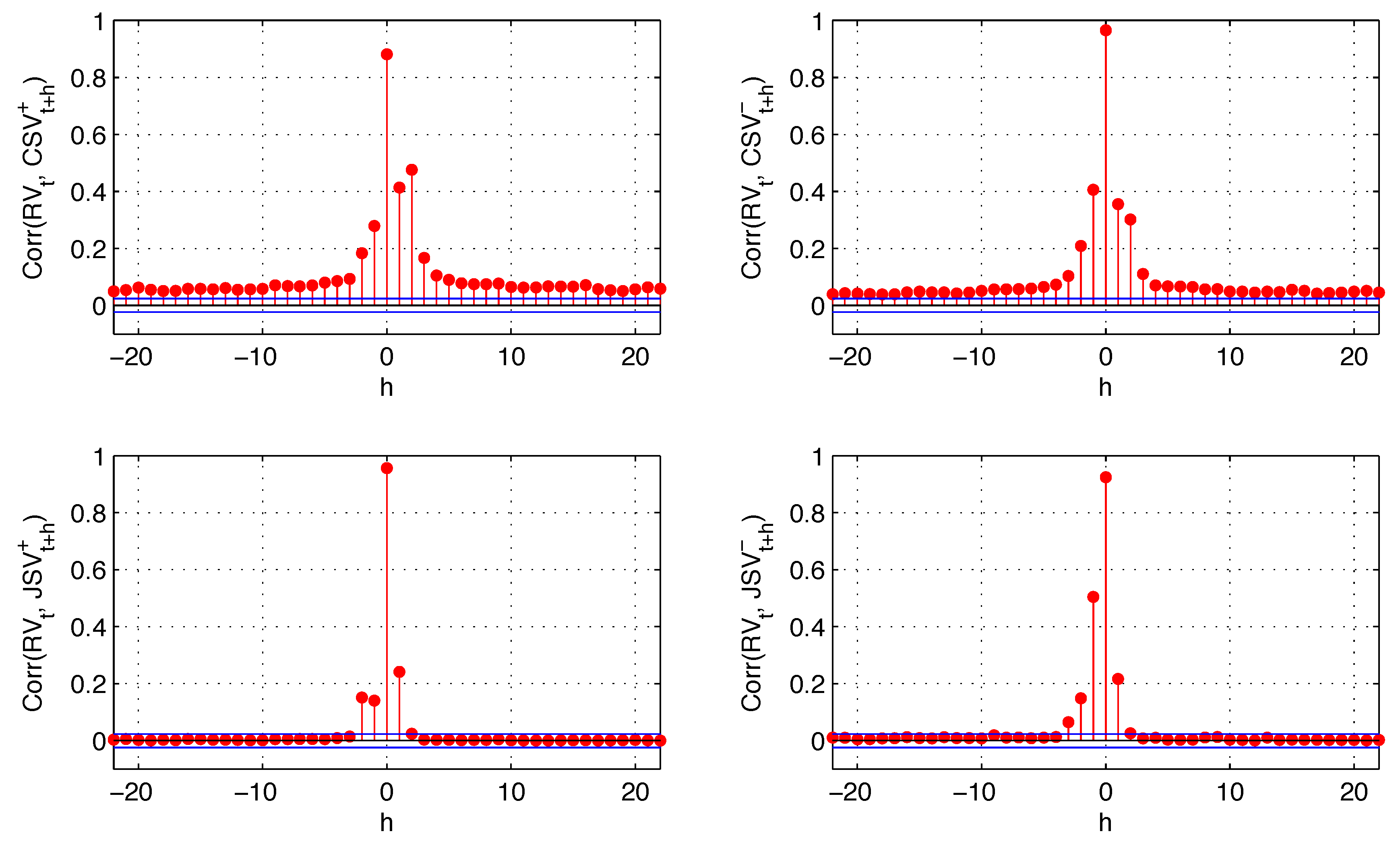
The persistence in volatility is also examined. It is well known that volatility is autocorrelated for a prolonged period of time. Evidence is found in [30] for the S & P500 stock index. Models to capture the persistence in conditional volatility have been proposed in their early stage by Engle, R.F. and Bollerslev, T. [31] and Baillie, R.T. et al. [32]. This autocorrelation is one of the drivers of the volatility feedback effect. The interpretation is that when an increase in volatility is associated with an expectation of higher future volatility, market participants may discount this information, resulting in an immediate drop in stock prices. We find that the persistence in volatility is mainly generated by the continuous component of the return variation. Jump variation has an effect on realized variance, as well, but this effect is short lived. The cross-correlations of realized variance with continuous variation and with jump variation are reported in Figure 5.

The quarter variances represent different sources of risk: positive and negative quarter variances represent “good” and “bad” risks, while continuous and jump quarter variances represent “expected” and “unexpected” risks. At a short horizon, they all have an impact on future volatility when they happen, while the persistence of this effect is mainly due to expected risks.

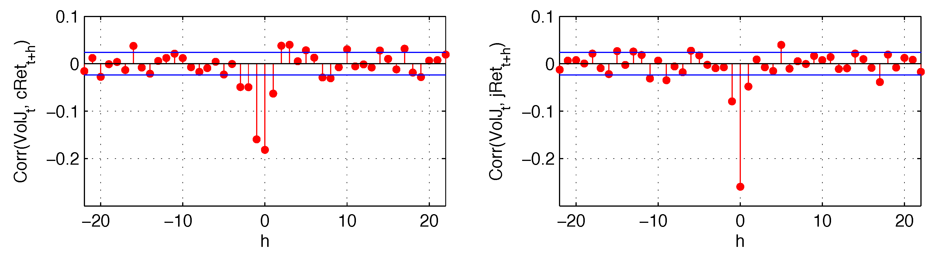
Finally, in Figure 6, we analyze the cross-correlation of both continuous and jump returns with the estimated volatility jumps. Both of those components are negatively and contemporaneously correlated with volatility jumps, with correlation between the two jump components reaching almost $-0.3$. Continuous and jump returns also have a short-lived impact on future volatility jumps. These results suggest that the leverage effect is also transmitted to the jump part of the variance. Consequently, the realized variance that we forecast consists of both continuous variation and jump variation, with the continuous variation not readjusted for volatility jumps.

4.2. In-Sample Analysis

Estimation results of the proposed forecasting models are discussed in this section. The in-sample evaluations are based on different horizons. The regression results of the candidate models are reported in

Table 2. The table contains estimates of the coefficients and t-statistics, in square brackets, based on Newey-West $HAC$ consistent standard errors, for the two model specifications. Model 1 and Model 2 correspond to Equations (28) and (29), respectively. The models are estimated for forecasting horizons of 1, 5, 15 and 22 days.

Horizon	Model	Variables
		Cons	CSV+	CSV-	JSV+	JSV-	VolJ	cRet-	cRet- (t-5,t]	jRet	RV (t-5,t)	RV (t-22,t)	adj-R2
1 day	1	0.030	0.137	0.146	-0.074	0.195	-0.001	-0.194	-0.173		0.330	0.263	0.727
		[1.16]	[6.29]	[7.41]	[-0.91]	[2.17]	[-0.04]	[-9.6]	[-4.44]		[10.64]	[11.37]
	2	0.098	0.158	0.136				-0.237		-0.099	0.375	0.235	0.726
		[4.89]	[7.78]	[7.1]				[-14.66]		[-2.64]	[12.92]	[10.59]
5 days	1	-0.004	0.113	0.088	-0.089	0.092	0.035	-0.125	-0.128		0.321	0.349	0.798
		[-0.14]	[7.01]	[5.44]	[-1.49]	[1.69]	[1.26]	[-7.48]	[-3.29]		[8.37]	[10.61]
	2	0.047	0.13	0.082				-0.157		-0.053	0.352	0.328	0.797
		[2.27]	[8.39]	[5.28]				[-10.39]		[-2.21]	[9.73]	[10.29]
15 days	1	-0.064	0.096	0.05	-0.061	0.061	0.043	-0.089	-0.130		0.271	0.413	0.777
		[-1.92]	[6.09]	[3.14]	[-1.19]	[1.39]	[1.74]	[-6.92]	[-2.75]		[6.23]	[9.58]
	2	-0.010	0.113	0.046				-0.123		-0.034	0.301	0.392	0.776
		[-0.35]	[6.92]	[2.83]				[-7.1]		[-1.84]	[7.15]	[9.11]
22 days	1	-0.078	0.084	0.044	-0.054	0.051	0.046	-0.080	-0.099		0.252	0.433	0.754
		[-2.13]	[5.42]	[2.62]	[-0.97]	[1.16]	[1.86]	[-6.3]	[-2.01]		[5.27]	[9.63]
	2	-0.034	0.099	0.042				-0.106		-0.026	0.273	0.416	0.754
		[-1.05]	[5.97]	[2.53]				[-5.97]		[-1.41]	[5.93]	[9.14]

, for horizons of 1, 5, 15 and 22 days. For multi-period forecasts, the predicted variable is the cumulative average log realized variance between time t and $t+h$.

In order to check the stability of the coefficients, regressions are run for different overlapping subsamples. As the full sample period is relatively long, consisting of more than 28 years, it is likely that structural breaks have occurred. This seems to be the case, as some coefficients estimated by including data for the initial eight years, from 1982 to 1989 (the forecasts are relative to the period 1990 to 1997), appear to differ from those estimated by using data starting from 1990. Conversely, the coefficients associated with the model for the last 20 years are relatively stable. 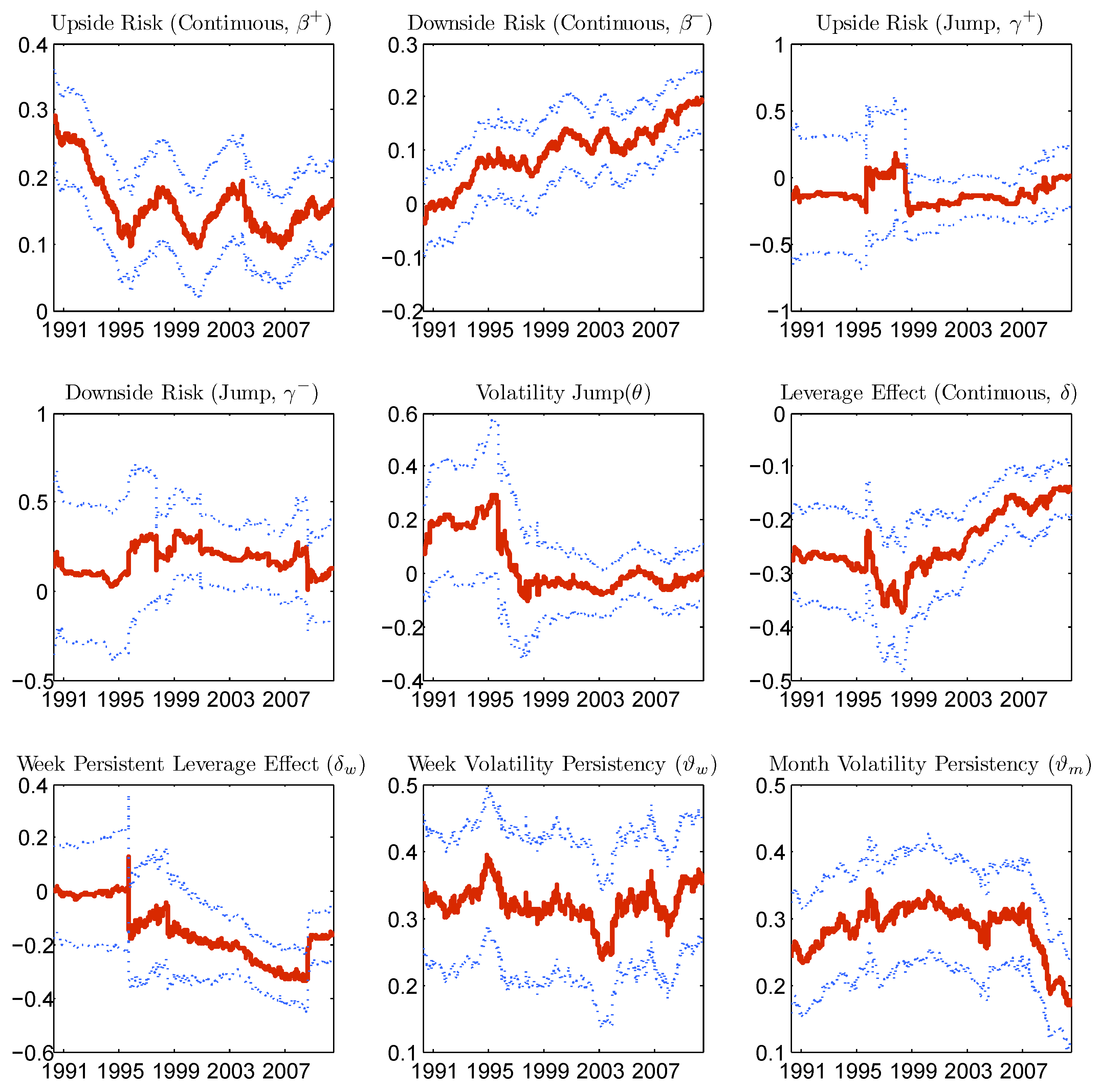Figure 7 reports the estimated coefficients of one period forecast of Model (28) with rolling subsamples of 2000 observations (corresponding to almost eight years).

With an in-depth inspection, the difference of the coefficient estimates for the initial subsamples from those of the remaining subsamples is mainly caused by the market crash of October 1987. The sample period is therefore reduced, and the results of the in-sample analysis contained in Table 2 are relative to the subperiod from 4 January 1988 to 6 August 20107. By contrast, the out-of-sample evaluations of the next sections, as they are performed using rolling forecasts, will be based on the whole sample period. Volatility jumps have a marginal power to forecast the one period ahead volatility only with the initial subsamples, which contain the market crash data, while for the remaining subsamples, they do not add further value. This indicates that volatility jumps are useful for forecasting during extremely agitated periods.

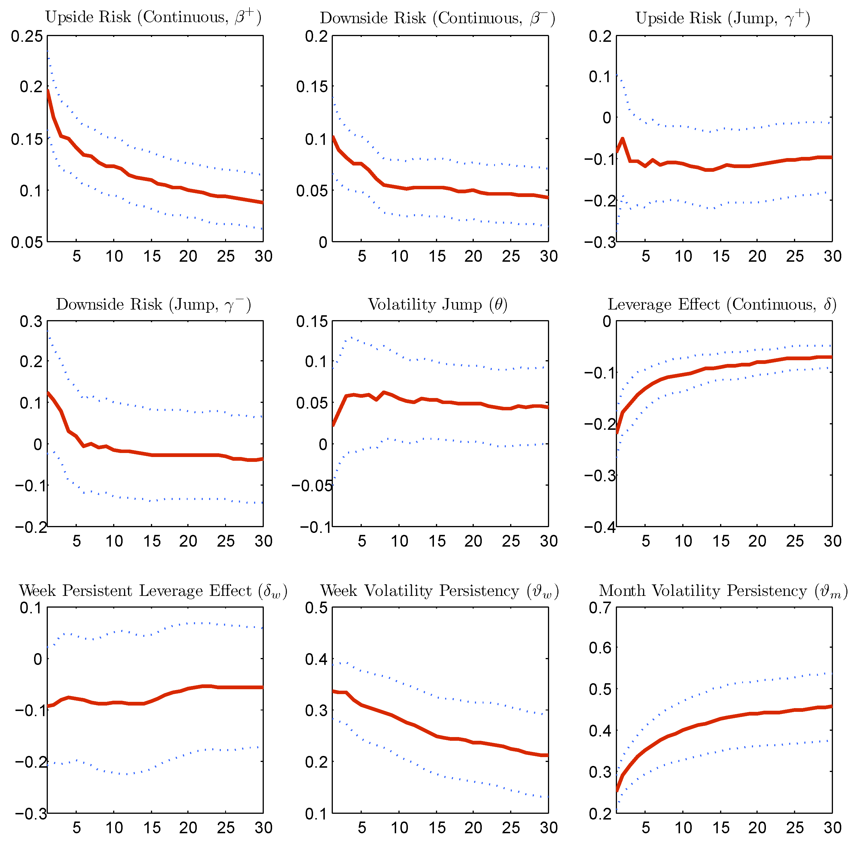
To check the stability of the estimates for different forecasting horizons, Figure 8 reports the estimated coefficients for forecasting horizons ranging from one day to 30 days. The estimated parameters appear to be well behaved. The major differences between the coefficients for the different forecasting horizons lie in the horizon of one to five days, while after five days, all of the estimates of the coefficients are stable. This stability is due to the fact that we predict the average cumulative variance over multiple periods.

The following results from the estimation are worthy of comment. “Bad risks” have a significant impact on future volatility. In fact, both continuous and jump downside quarter variances increase future realized variance. However, when “good risks” are disentangled into upside continuous and jump quarter variances, a striking difference emerges. The effect of upside continuous variance on future volatility is still positive and statistically significant, but that of the upside jump variance is on average negative and negligible. This may well answer the critique advanced by Corsi, F. et al. [24], as they argue that influential studies, such as [5] and [33], among others, find a negative or null impact of jumps (more appropriately jump variation) on future volatility, while economic theory suggests the opposite. In fact, one needs to distinguish between downside and upside jumps. Future volatility is indeed increasing with downside jump variation, as jump variations are likely associated with an increase in uncertainty on fundamental values. However, the effect of upside jump variation does not necessarily increase future volatility. This would be consistent with the economic model of [34]. Intuitively, a positive jump is associated with the occurrence of good news, as well as the expectation of higher future returns. The effect of the latter is able to offset the effect of an increasing uncertainty. The future volatility given the occurrence of a positive jump is therefore lower than the one associated with the occurrence of a negative jump.

Consistent with the leverage effect, both continuous and jump components of the return have a significant impact on future volatility. As mentioned previously, the persistence in leverage effect is captured mainly by the continuous component. In fact, as the forecasting horizon increases, the leverage effect generated by past jumps becomes less statistically significant. On the contrary, either coefficients associated with the negative continuous return over the past day and over the past week remain statistically significant even for longer forecasting horizons.

Concerning long memory features, the persistence parameters associated with the one week and the one month realized variance terms are both highly statistically significant for all horizons. Ultimately, jumps in volatility (continuous variation) do not appear to be statistically significant. Given that volatility jumps are present during extremely agitated periods, their null forecasting performance on the short horizon is due to the fact that only a few volatility jumps are identified for the sample period under investigation. There are in fact volatility jumps for only 3.6% of the sample days.

Finally, by examining the (in-sample) performance of the simplified Model (29) in comparison with that of the full model, the losses in accuracy that occur for the simplified model are negligible based on the adjusted $R^2$.

4.3. Out-of-Sample Forecasting Performance

The methodology used to assess the forecasting performance of the proposed models is presented in this section. The analysis is based on the out-of-sample predictive accuracy of these models in comparison to the $HAR-RV$ Model (26). The predicted variable is the cumulative average log realized variance between time t and $t+h$. For predictions of horizons $h>1$, a “direct method” is employed, that is the model specifies only the relation between $log{\left(RV\right)}_{t,t+h}$ and the regressors at time t. The evaluation of the performance is done recursively with rolling windows. The forecasting horizons considered are $h=\left\{1,5,15,22\right\}$.

The recursive procedure is applied as follows: The forecasts are generated by using an in-sample estimation window of 2000 observations, corresponding to about eight years, starting from 28 April 1982. For $h=1$, the performance is evaluated on 5040 out-of-sample data points, corresponding to about 20 years. The forecasting performance is based on the $MSE$ function of the log realized variance forecasts and the negative $QLIKE$ loss function:

$$\begin{array}{cc}\hfill MSE& ={\left(\widehat{ln{\left(RV\right)}_{t,t+h\mid {\mathcal{F}}_t}}-ln{\left(RV\right)}_{(t,t+h]}\right)}^2,\hfill \end{array}$$

(30)

$$\begin{array}{cc}\hfill QLIKE& =\widehat{ln{\left(RV\right)}_{t,t+h\mid {\mathcal{F}}_t}}+\frac{R{V}_{(t,t+h]}}{\widehat{R{V}_{(t,t+h]\mid {\mathcal{F}}_t}}}.\hfill \end{array}$$

(31)

The $MSE$ is a symmetric loss function, while $QLIKE$ is asymmetric. The work in [35] shows that the $QLIKE$ loss function is robust to noise in the volatility proxy, as volatility forecasts represent a case where the true values are not observable. Moreover, this function has certain optimal properties in that it is less sensitive to large observations by more heavily penalizing under-predictions than over-predictions. It is therefore more suited to yield model rankings in the presence of imperfect proxies.

To test for the superior forecasting performance of the proposed models over the benchmark $HAR-RV$ model, the [36] test is employed. The asymptotic variance of the loss differential (of each model and the $HAR-RV$ model) is estimated with Newey-West $HAC$ consistent sample variance, as suggested by Giacomini, R. et al. [37]. The work in [38] shows that in the presence of nested models, the distribution of the Diebold-Mariano test statistics for mean square error losses, under the null, can be nonstandard. Therefore, the test of forecasting performance for mean square error losses is based on the [39] test statistic, which appropriately corrects the loss differential.

Table 3. The table reports results from the out-of-sample pairwise forecast performance comparison. The performance is based on the $QLIKE$ and $MSE$ loss functions for Models 1 and 2 corresponding to Equations (28) and (29), respectively. Each model is evaluated against the benchmark $HAR-RV$ (Equation 26). Forecast horizons considered are 1 day, 5 days, 15 days and 22 days. The upper panel reports the Diebold-Mariano t-statistics on $QLIKE$ losses, and the bottom panel reports the Clark-West test statistics on $MSE$ losses. The out-of-sample performance period ranges from May 1990 to August 2010.

	Model	Horizon
		1 day	5 days	15 days	22 days
DM Test Statistics with QLIKE Losses	1	4.87	4.34	2.38	1.80
	2	4.44	4.65	3.16	3.13
CW Test Statistics with MSE Losses	1	11.34	10.83	7.72	6.67
	2	11.70	10.84	7.73	6.79

reports the test statistics under the null of equal forecasting performance for each model pair. A positive value represents the superior average forecasting performance of the proposed model with respect to the $HAR-RV$.

At the 99% confidence level, the proposed models outperform the base model for forecasting horizons of one day and five days. For longer forecasting horizons, overall, the models also perform well, with the reduced model (Equation (29)) achieving surprisingly high performance. Based on the $QLIKE$ loss function, the out-performance of the full Model (28) compared to the $HAR-RV$ model is only weakly statistically significant. This is a warning signal that Model (28) is probably over-parametrized, although as shown in the next section, outperforming the benchmark $HAR-RV$ model in forecasting long-run volatility seems to be a difficult task.

4.4. Model Confidence Set

The $HAR$ model in logarithmic form generally has a good out-of-sample forecasting performance. In an attempt to raise the bar, other reference models recently proposed in the literature are considered. First, we test the performance of the $HAR$ model for the realized variance, which yielded the lowest forecasting power among all of the candidate models when evaluated on the loss functions Equations (30) and (31). Then, we investigate the accuracy of the variance forecasts for several models involving two model specifications of [5] (Equation (13), p. 709, and Equation (28), p. 715), named $HAR-RV-J$ and $HAR-RV-CJ$, respectively, which explicitly take into account continuous and jump variation; two specifications proposed by Patton, A.J. and Sheppard, K. [7] (Equation (19), p. 16, and Equation (17), p. 13, without upside semi-variance) based on upside and downside variances, one with complete decomposition into quarter variances and the other with a downside quarter variance only for the daily component; and two models of [6] (Equation 2.4, p. 8, and Table 3, p. 16) that add the leverage effect, named $LHAR-CJ$ and $LHAR-CJ+$, respectively. Finally, simple and commonly-used models are also taken into account. These are an autoregressive model on the daily log realized variance component only and an exponential smoothing model. The last is popularly used by risk practitioners (see [40]) and is specified as

$$\widehat{log{\left(RV\right)}_{(t,t+h]}}=\alpha ·log{\left(RV\right)}_{(t-h,t]}+\left(1-\alpha \right)·\widehat{log{\left(RV\right)}_{(t-h,t]}}$$

(32)

with parameter α optimized for each rolling window following

$$arg\underset{\alpha }{min}\sum _t\left[log{\left(RV\right)}_{(t-h,t]}-\widehat{log{\left(RV\right)}_{(t-h,t]}}\right].$$

All of the models (except the $HAR-RV$) are evaluated on log realized variance. They are also estimated on the same rolling window and evaluated on the same out-of-sample data points. It is also worth mentioning that jump detection and quarter variance estimation are executed in the same way as described in this article.8

In order to evaluate forecasts of those models, the model confidence set ($MCS$) methodology of [41] and [42] is the most well suited. The comparison is done among a set of models, as pairwise comparisons would not be appropriate. The methodology allows the models to be ranked based on a given loss function, and it gives an indication of whether the forecast performances are significantly different. Out of the surviving models in the confidence set, the interpretation is that they have equal predictive ability, and they yield the best forecasts given a confidence level.

The model confidence set approach allows the user to specify different criteria to establish equal forecasting performance for the model set and subsets. We use both the “range” statistic and the “semi-quadratic” statistic:

$$\begin{array}{ccc}\hfill T_R& =& \underset{k,s\in M_{set}}{max}\frac{\left|{\overline{d}}_{k,s}\right|}{\sqrt{\widehat{var}\left({\overline{d}}_{k,s}\right)}},\hfill \end{array}$$

(33)

$$\begin{array}{ccc}\hfill T_{SQ}& =& \sum _{k,s\in M_{set}}\frac{{\overline{d}}_{k,s}^2}{\widehat{var}\left({\overline{d}}_{k,s}\right)},\hfill \end{array}$$

(34)

where ${\overline{d}}_{k,s}$ is the mean loss differential between each pair combination of models, with k and s denoting each model.

Table 4. The table reports the forecasting performance of models in the confidence set. A block bootstrap procedure with 5000 replications is used to establish equal predictive ability of the surviving models according to both “range” and “semi-quadratic” test statistics. Moreover, both $QLIKE$ and $MSE$ (on log realized variation) losses are used. Forecast horizons considered are 1 day, 5 days, 15 days and 22 days. “+” denotes included models in the final confidence set with significance level 5%, and “++” denotes included models in the confidence set with significance level 10%, with $MC{S}_{10\%}\subseteq MC{S}_{5\%}$. Models 1 and 2 correspond to Equations (28) and (29), respectively.

Model	Statistics	QLIKE Loss Function Forecasting Horizon				MSE Loss Function (on log RV) Forecasting Horizon
		1 Day	5 Days	15 Days	22 Days	1 Day	5 Days	15 Days	22 Days
HAR (log RV)	Mean loss (Full Sample)	0.524	0.453	0.455	0.465	0.260	0.158	0.163	0.176
	MCS (R-Stat)
	MCS (SQ-Stat)			+	++			+	++
HAR (RV)	Mean loss (Full Sample)	0.614	0.682	0.743	0.773	0.650	0.629	0.661	0.682
	MCS (R-Stat)
	MCS (SQ-Stat)
Mod. 1	Mean loss (Full Sample)	0.514	0.449	0.453	0.463	0.245	0.152	0.159	0.174
	MCS (R-Stat)	++	++	++	++		++	++	++
	MCS (SQ-Stat)	++	++	++	++		++	++	++
Mod. 2	Mean loss (Full Sample)	0.515	0.449	0.453	0.463	0.244	0.152	0.159	0.173
	MCS (R-Stat)	++	++	++	++	+	++	++	++
	MCS (SQ-Stat)	++	++	++	++	+	++	++	++
Semivariances - HAR 1 (PS, 2011)	Mean loss (Full Sample)	0.521	0.452	0.456	0.466	0.255	0.157	0.163	0.178
	MCS (R-Stat)
	MCS (SQ-Stat)			++	+			++	++
Semivariances - HAR 2 (PS, 2011)	Mean loss (Full Sample)	0.521	0.452	0.455	0.464	0.255	0.156	0.162	0.176
	MCS (R-Stat)
	MCS (SQ-Stat)			++	++			++	++
HAR-RV-J (ABD, 2007)	Mean loss (Full Sample)	0.524	0.453	0.455	0.465	0.259	0.158	0.162	0.176
	MCS (R-Stat)
	MCS (SQ-Stat)			+	++			++	++
HAR-RV-CJ (ABD, 2007)	Mean loss (Full Sample)	0.524	0.452	0.455	0.465	0.258	0.157	0.161	0.176
	MCS (R-Stat)			++				++
	MCS (SQ-Stat)			++	++			++	++
LHAR-CJ (CR, 2010)	Mean loss (Full Sample)	0.513	0.449	0.454	0.464	0.242	0.151	0.160	0.175
	MCS (R-Stat)	++	++	++	++	++	++	++	++
	MCS (SQ-Stat)	++	++	++	++	++	++	++	++
LHAR-CJ+ (CR, 2010)	Mean loss (Full Sample)	0.513	0.449	0.454	0.464	0.242	0.151	0.160	0.175
	MCS (R-Stat)	++	++	++	++	++	++	++	+
	MCS (SQ-Stat)	++	++	++	++	++	++	++	++
Autoregressive 1 day	Mean loss (Full Sample)	0.562	0.502	0.513	0.524	0.325	0.247	0.265	0.282
	MCS (R-Stat)
	MCS (SQ-Stat)
Exponential Smoothing	Mean loss (Full Sample)	0.527	0.460	0.774	0.490	0.265	0.170	0.192	0.210
	MCS (R-Stat)
	MCS (SQ-Stat)

reports the model confidence set and the selected models at the classic 5% and 10% significance levels. The model confidence set p-value is obtained through a block bootstrap procedure. An autoregressive process is estimated for each $d_{k,s}$, the loss differential between each model k and s and the lag length, for it is determined by Akaike information criteria, as suggested by Hansen, P.R. et al. [41]. The block length for the bootstrap procedure is then fixed as the maximum lag length among $d_{k,s}$, and it varies between nine and 30 depending on the forecasting horizon and the loss function used. Five thousand bootstrap repetitions are used to compute the test statistics. The model confidence set p-value obtained by using the semi-quadratic test statistics is less conservative than the one obtained by using the range statistics. The surviving model set after using the semi-quadratic test statistic is therefore larger than the set obtained by using the range test statistic.

Overall, the best forecasting models for all different horizons are the candidate Models (28) and (29) and the two $LHAR-CJ$ models proposed by Corsi, F. et al. [6], which take into account past negative return without disentangling return jump size. The reduced model of Equation (29) achieved equal forecasting performance, compared to the $LHAR-CJ+$ model, with a lower model complexity (four variables less). Jumps in return indeed substantially improve the forecasting performance, while volatility jumps are infrequent and have a minor effect on future realized variance. For the one period ahead forecast, the full Model (28), which includes volatility jumps, does not survive based on the $MSE$ loss function. However, it does survive based on the $QLIKE$ loss function. This is due to the fact that by adding volatility jumps, the model tends to produce marginally less conservative forecasts of volatility. The $QLIKE$ loss, since it less heavily penalizes over-predictions than under-predictions, still selects this model. Finally and not surprisingly, the best forecasting models are the ones that include the leverage effect.

The following considerations can be pointed out for the simplest models: for long horizons, the simple $HAR-RV$ model is hard to beat. As has already been shown in the literature, the autoregressive model that takes only the daily component into account is not selected for any forecasting horizon and loss function used, pointing to the importance of correctly modeling long memory. Moreover, the exponential smoothing model, often used in practice, is clearly outperformed.

5. Conclusions

This paper analyzed the performance of volatility forecasting models that take into account downside risk, jumps and the leverage effect. The volatility forecasting model proposed consists of the following ingredients: First, the timing and the size of intraday return jumps is estimated based on the jump test of [8]. Second, jump variation and continuous variation are disentangled into signed quarter variances using signed intraday returns. Finally, the size of jumps in volatility is also estimated with inference based on an auxiliary $AR-GARCH$ model. The best candidate model for forecasting realized variance must simultaneously take into account return jumps, “good” and “bad” risks, leverage effect and strong volatility persistence (i.e., long memory).

The model is motivated by the overwhelming empirical evidence of asymmetries in financial time series. We show that correlation asymmetries are present for both continuous and jump components among return and volatility. Moreover, asymmetries exist not only in size, but also in sign, justifying the use of quarter variances in forecasting volatility. Finally, the persistence of the volatility leverage effect is mostly due to the continuous returns.

The forecasting model is very simple to implement, as it is based on the parsimonious $HAR$ framework. The gain over the base $HAR-RV$ in terms of out-of-sample forecasting power is substantial, and this is especially true for short and mid- forecasting horizons. However, for an accurate identification of jumps and the estimation of the jump size, the availability of high frequency data is required. In fact, the empirical analysis is based on a long history of high frequency S & P500 Futures data. When enough high frequency data are available, the effort of estimating return jumps and signed quarter variances is compensated with generally better predictions of future volatility.

Considering that synthetic instruments with financial market implied volatility (e.g., VIX index) as the underlying asset have existed for decades and that the use of the realized volatility itself as a market index is also becoming popular, the methodology proposed can be applied directly to construct profitable trading strategies that apply leading indicators based on quarter variances and jumps. In such applications, given the need for a long history of data and the possible presence of structural breaks, the forecasting model must be re-trained often to obtain accurate predictions. In this article, for example, for the out-of-sample forecast performance evaluation, we re-estimated the model every day using a rolling window strategy. Moreover, depending on the investment horizon and the economic objective of the trading strategy, for instance a minimum return strategy within a period of time or a “no-big loss” strategy, the forecasting model can be selected based on variants of the “MSE” or “QLIKE” loss functions used in this paper or other direct economic evaluation methods.