We report distributions of biases instead of means, variances and/or mean squared errors because of the possible non-existence of the second (and even first) moments for these distributions.
Appendix B ‘Selected Bias Distributions’ shows noteworthy graphs representative of the results; an online Appendix at
is.gd/vartarget contains a more complete collection of graphs (see the table with the description of experiments in its preamble), as well as tables with their numerical representation. Of primary interest is a median bias as the most appealing characteristic of the bias of estimated objects. See Andrews [
25] who made forceful arguments about the practical appeal of the notion of median-unbiasedness, especially “when the parameter space is bounded or when the distributions of estimators are skewed and/or kurtotic,” the circumstances we face here.
3.1. Parameter Biases
In this subsection, we present the results on parameter biases
given by (
20) and expressed in percentages, from QML estimation in the skewed Student GARCH model in the following order:
,
,
,
and
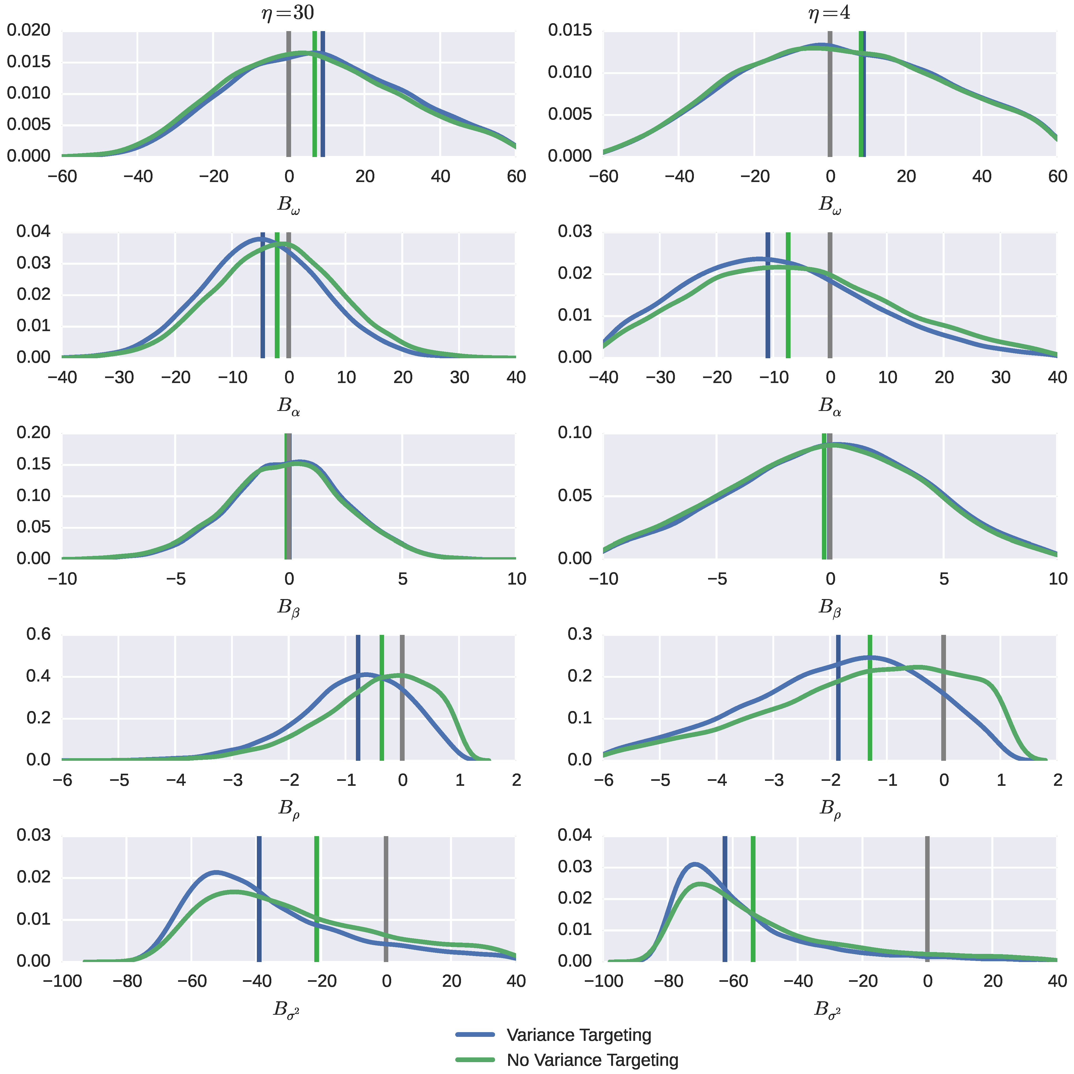
. Their distributions are partly shown in
Figure 3; more graphs are available in the online Appendix as Figures A.1–A.5. The axes are expressed in percentages to true parameter values. In
Figure 3, the two columns correspond to two selected values of the degrees of freedom parameter
η representing almost mesokurtic (
) and highly leptokurtic (
) standardized return distributions, while the five rows correspond to five parameters; the value of the feedback parameter
β is fixed at 0.8. In Figures A.1–A.5, the two columns correspond to two values of the feedback parameter
β, while the five rows correspond to five values of the degrees of freedom parameter
η. The blue lines correspond to variance targeting, the green lines to “regular” QML estimation. The vertical lines of corresponding color are placed at the medians of distributions; in addition, gray vertical lines are placed at zero, the ideal value of a bias. Correspondingly, Tables A.1–A.5 contain 5%, 25%, 50%, 75% and 95% percentiles, expressed in percentages to the true parameter value, of bias distributions. Recall that throughout,
and
(implying
).
The estimates of the intercept ω are not severely median biased: the maximal reported median bias corresponds to an about 13% deviation from the true value. The median bias is positive, smaller for the smaller value of β and always bigger when variance targeting is used, although by a narrow margin. The shape of the bias distribution is similar in the cases of variance targeting and of no variance targeting and so is its dispersion. The median bias stays stable (or goes up very slowly) when the return distribution becomes heavier tailed, but sharply drops down when the tails become so heavy that the higher moments of the standardized error distribution fail to exist. The dispersion goes up significantly with heavy tailedness for both methods: the inter-percentile range approximately doubles when the return distribution turns from mesokurtic to strongly leptokurtic. The maximal reported 95% percentile corresponds to an estimate that is higher than triple the true value.
The median bias for the news impact parameter α is negative and is again larger in absolute value when variance targeting is used, up to twice as large, although the discrepancy in relative terms falls with the degree of heavy tailedness. In contrast to median biases for ω, it is larger for the smaller value of β (and hence, the bigger value of α). The median bias, importantly, increases (in absolute value) with the degree of return leptokurtosity pretty quickly. However, even for highly tailed return distributions, the median bias is relatively moderate (maximum 20%) if contrasted to the bias dispersion, which is big in both cases: the percentile can exceed 120%. It tends to be bigger when no variance targeting is used, though not significantly, and bigger for the smaller value of α.
The median bias of estimates of the feedback parameter β is practically non-existent (which is natural given its high identifiability), whether the return distribution is thin or thick tailed and whether variance targeting is used or not; it amounts to less than half a percent in absolute value, even when the distribution is very leptokurtic. However, the tails of the distributions and their dispersion steadily rise with the degree of return leptokurtosity. The left tail is about twice as long as the right tail.
The relative bias of estimates of the persistence parameter ρ is of a similar magnitude as that for β, the median bias being of order of a few percent, despite the fact that estimation of the other ingredient of the sum, α, may be subject to substantial biases. This happens because in absolute terms, α is (as typically) much smaller than β, whose estimation is subject to a very small median bias. The median bias is always negative, larger (in absolute value) for the smaller value of β and moderately increasing in the degree of return leptokurtosity. It is larger when variance targeting is used than when it is not, though not appreciably. As far as the dispersion is concerned, it is inherited from those in the estimation of both β and α in such a way that most probability weight is put on the left tail, which is quite long and heavy. The right tail of bias distributions are bounded because of an implicitly-embedded condition on ρ not to exceed unity.
Last, but not least, and in fact most importantly, one can see that estimates of the unconditional variance
exhibit severe biases
12 compared to those of the other parameters. Even the median bias reaches and well exceeds (in absolute value) 50% in some cases. It steadily goes up with the degree of return leptokurtosity and is noticeably larger for the smaller value of
β. The bias distribution quickly shifts leftward as the degree of return leptokurtosity increases. When variance targeting is used, the median bias is much larger, up to twice as much, although the discrepancy in relative terms falls with the degree of heavy tailedness, and when the tails are very thick, the difference is not so impressive. The larger median bias under variance targeting may sound surprising, as the estimate in this case is just that of the method-of-moments, which is mean unbiased (but highly skewed and, thus, severely median biased) and does not use the GARCH model at all. Exploitation of the model imposing the connection between the model parameters in the likelihood function significantly reduces the median bias, though making the bias distribution much more dispersed, primarily in the right tail. The latter fact is explained by a high frequency of estimates of
ρ that get close to unity and make the estimate of
unstable; this phenomenon, naturally, becomes weaker when the persistence is not so strong.
To conclude, parameter estimate biases are strongly and positively related to the heaviness of the tails of the return distribution. Among the model parameters, it is the unconditional variance that experiences the severity of estimation bias most, with the intercept coming next. However, that severity is qualitatively different when variance targeting is used or not.
3.2. VaR Prediction Biases
Now, we analyze the bias of one-period and long-run value-at-risk predictions
and
defined in Equations (
23) and (
24), respectively. The biases of VaR predictions are inherited from the biases in the intercept
ω and the persistence parameter
ρ in the case of short-run prediction and from the biases in the unconditional variance
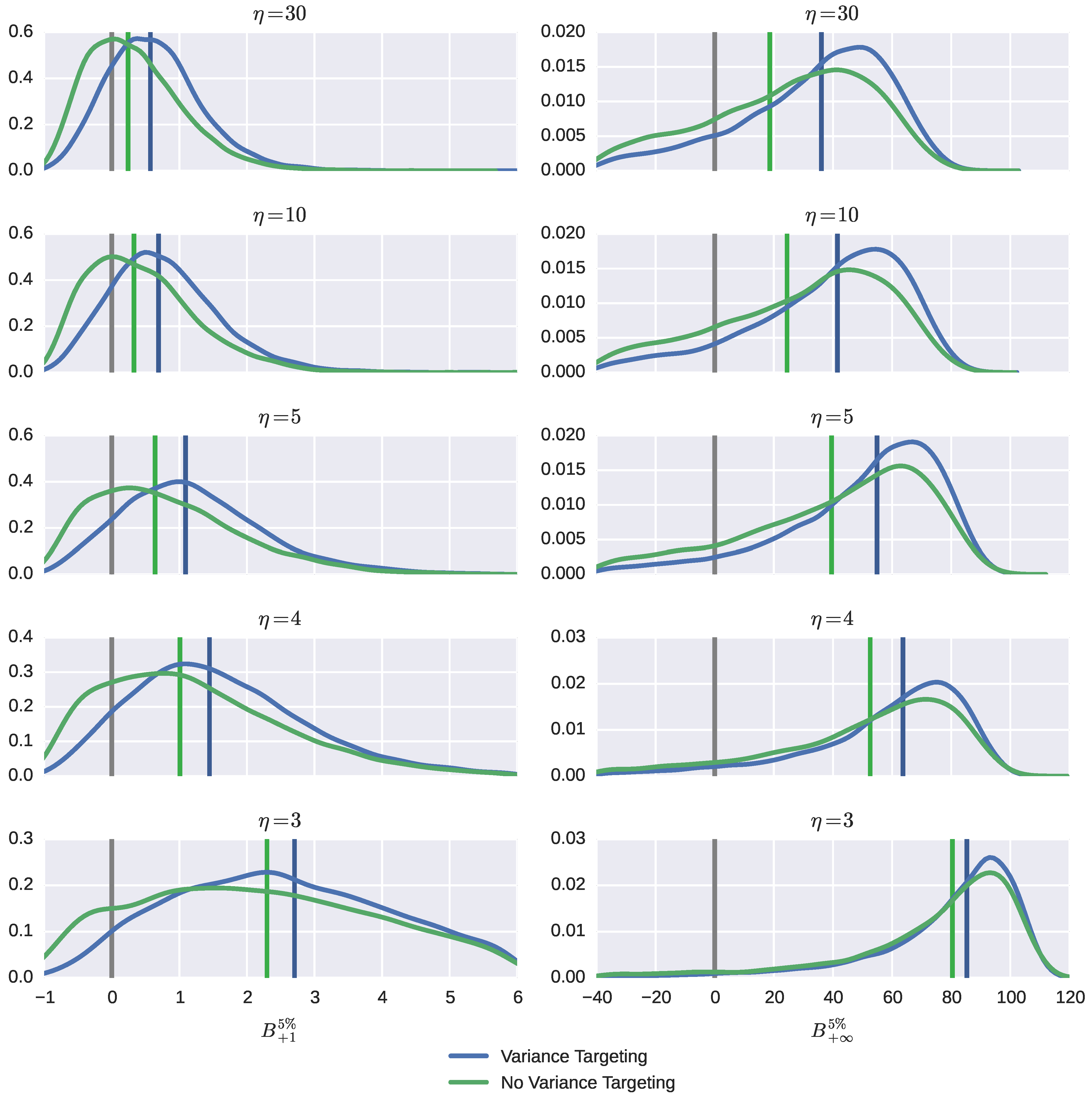
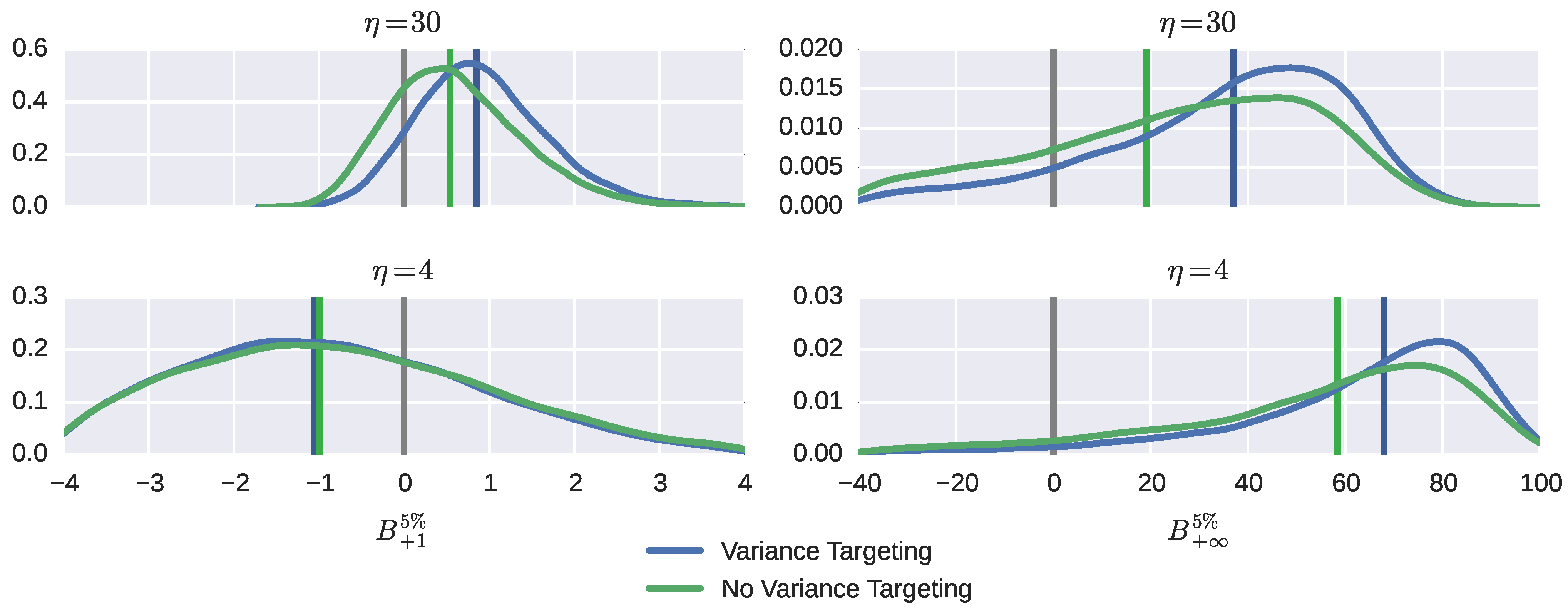
in the case of long-run prediction. From the previous analysis, it is clear that the behavior of biases is expected to be qualitatively different in the two cases. Their distributions are shown in
Figure 4 and more fully in Figures A.6–A.7, with numerical presentation given in Tables A.6–A.7. The format of the graphs and tables is the same as described before. In
Figure 4, the left column contains distributions for
and the right column for
.
One-period VaR predictions are the most frequently overpredicted, although the bias is quite small, except when the standardized return distribution is highly leptokurtic. This bias is driven mostly by the bias in the persistence parameter ρ, hence it is larger for the smaller value of β. The median bias rises with return leptokurtosity and becomes perceptible only for very heavy-tailed distributions of standardized returns. It is systematically larger when variance targeting is used, but by small amounts; the discrepancy almost vanishes when the standardized error distribution gets very thick tailed. The inter-percentile ranges are also quite similar.
However, the typical figures of the maximum mere a few percent, characterizing that the median biases for short-run VaR are incomparable to those for the long-run VaR, which can reach 50% and higher. This bias is driven entirely by the bias in the unconditional variance , hence such a result. The median bias is appreciably higher for the smaller value of feedback β. Under variance targeting, for mesokurtic standardized returns, the median bias is about twice as much as that without variance targeting. The median bias is increasing with the degree of thick tailedness and so do the inter-percentile ranges. An interesting phenomenon occurs when the degrees of freedom parameter η changes its value from four (implying the existence of conditional skewness, but the non-existence of conditional kurtosis) to three (implying the non-existence of either). When this happens, the distributions of VaR predictions (in addition to spreading out) shift rightward, leading to significant increases in either median bias. Overall, the bias is more dispersed when no variance targeting is used.
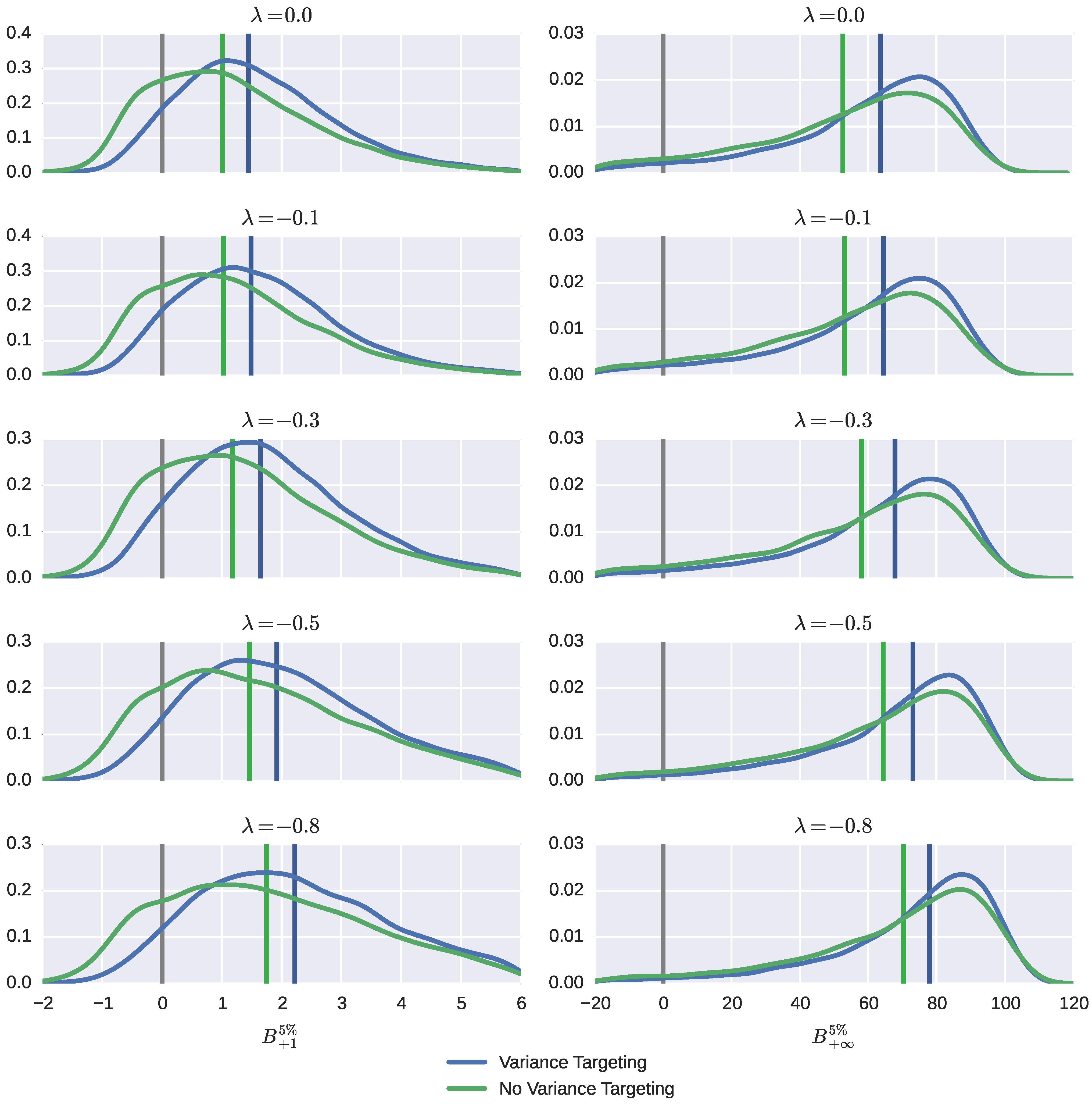
Next we analyze the impact of skewness of the return distribution on the bias. The evidence for the VaR criteria is shown in
Figure 5, while Figures and Tables B.1–B.7 give a more complete picture, including that for parameter estimates. The five rows now correspond to five values of the asymmetry parameter
λ; the degrees of freedom parameter is fixed at
, implying a highly leptokurtic distribution for standardized returns. As the degree of distributional asymmetry varies from zero up to extreme values, the distribution of the bias does change, but not very significantly. Biases in some parameters double and so do biases in short-run VaR predictions as a result. The unconditional variance
and, as a result, the long-run VaR predictions are subject to higher estimation biases when the return distribution becomes asymmetric, but this change is not too dramatic: the median bias goes up by less than 50% of its value.
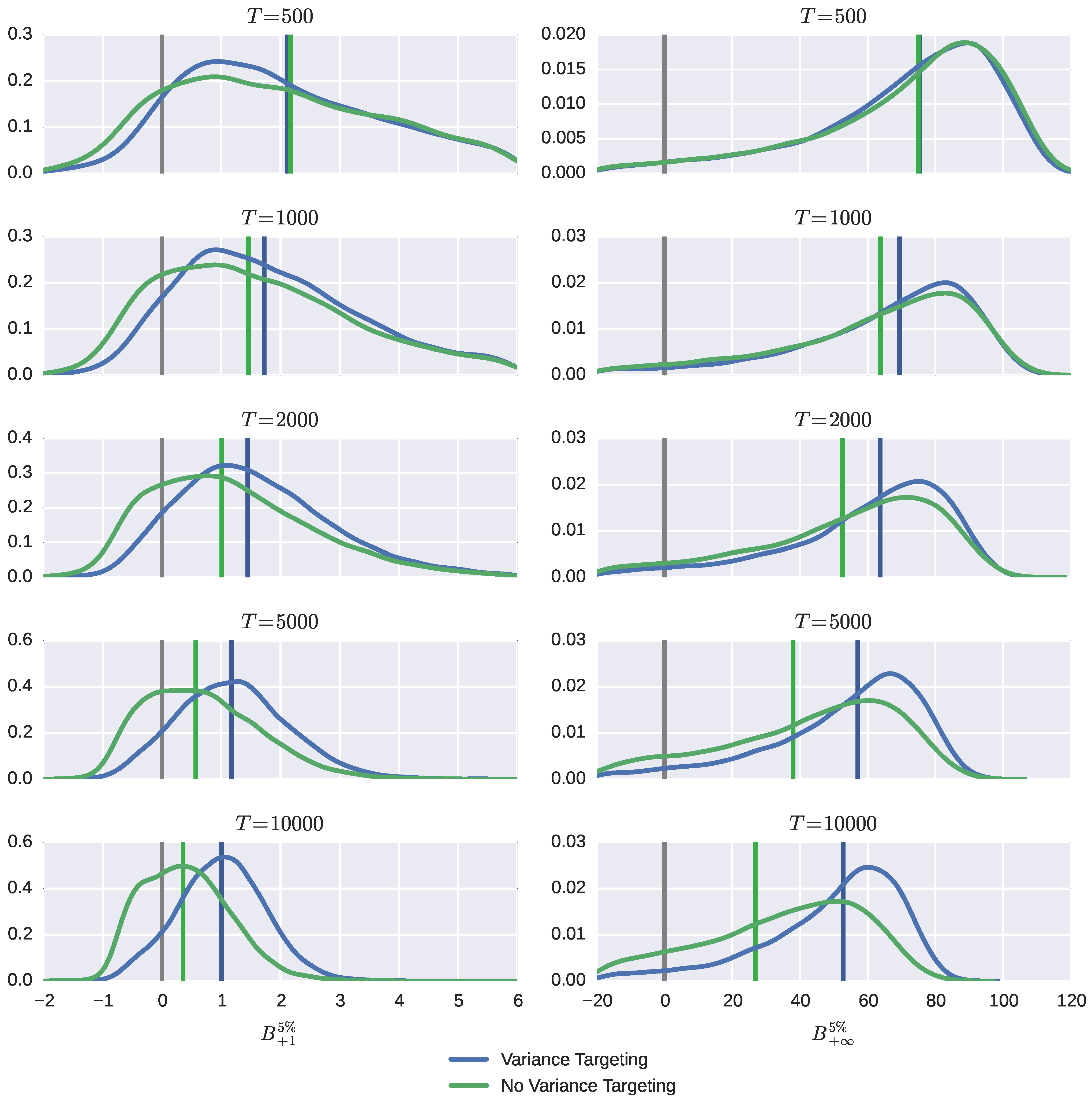
Recall that all previous evidence is given when the sample size
T equals 2000. Now, we analyze the impact of a sample size on the bias. The evidence for the VaR criteria is shown in
Figure 6, while Figures and Tables C.1–C.7 give more complete evidence, including that for parameter estimates. The five rows now correspond to five values of
T; the shape parameters are fixed at
,
implying a highly leptokurtic symmetric distribution for standardized returns. Note that for a very small (for typical financial series, about two years of daily data) sample size of 500, our previous conclusions are exacerbated. As
T increases, all biases naturally become substantially smaller, both in median and inter-percentile terms. However, this happens at a different rate depending on whether short- or long-run VaR predictions are considered and whether variance targeting is used or not. Overall, biases of short-run predictions tend to shrink faster than long-run counterparts and faster when no variance targeting is used than when it is used. Indeed, as
T rises by 20 times (note that
), while the median bias drops by 6–8 times or by 2–3 times, depending on the value of the feedback parameter under QML, it drops only by 3–5 times or 1.5–2 times, respectively, under variance targeting. However, QML predictions of long-run VaR predictions bear a significant risk of underprediction, even when sample sizes are quite large.
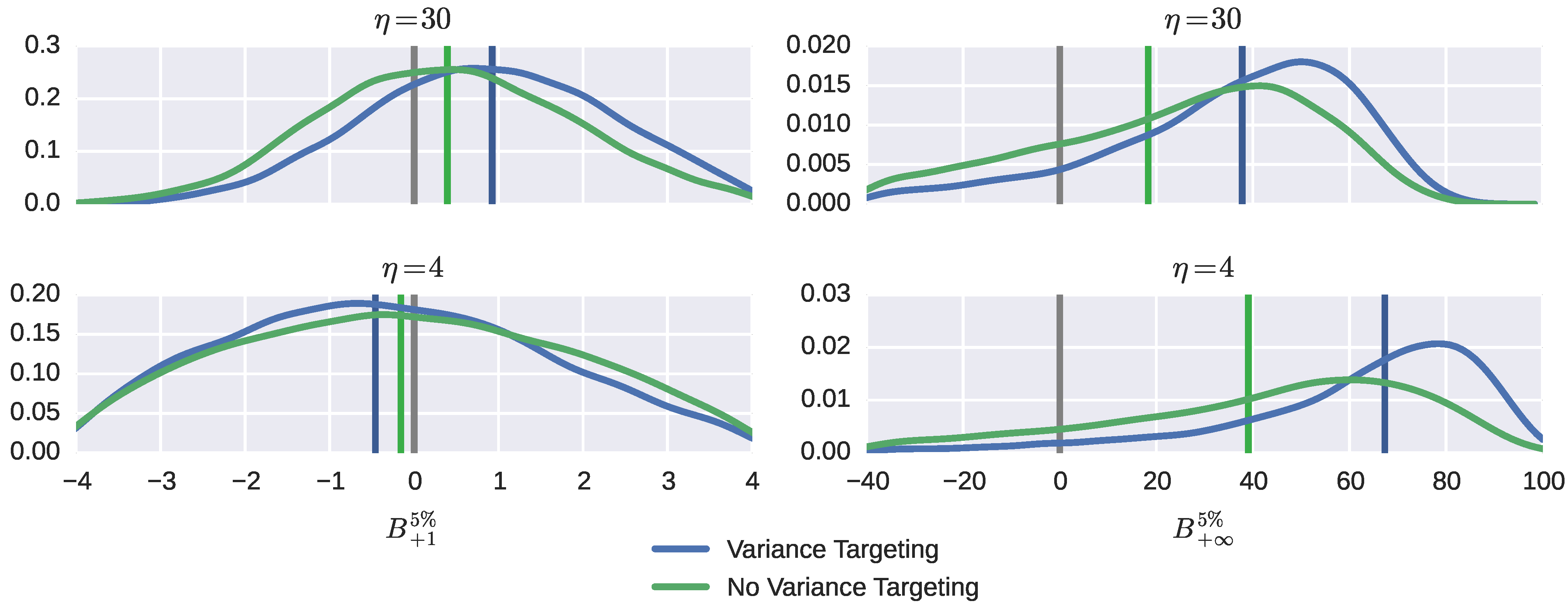
3.3. GJR in Place of GARCH
Next, we verify whether and how the presence of leverage effects in the volatility equation affects bias. The distributions of biases for selected parameters and VaR predictions are shown in
Figure 7. Figures and Tables D.1–D.8 contain more complete information; one can compare these to Figures and Tables A.1–A.8 and
Figure 7 to
Figure 3 and
Figure 4.
The bias properties of estimates of the news impact parameter α when leverage is present naturally deteriorate, as serial correlation features in squared returns (together with return signs) now need to identify two parameters α and γ at the same time; effectively, only (approximately) half of the sample is used for either. As a result, the (negative) median bias increases and so does bias variability. This effect is especially pronounced for the larger value of β and, hence, smaller value of α. However, the bias properties for the persistence parameter ρ do not significantly change, even though it contains both α and γ; evidently, persistence is identifiable as adequately with leverage effects as without them. The discrepancy in bias properties for α and γ between variance targeting and no variance targeting are similar, though noticeably magnified. The intercept parameter ω and feedback parameter β experience bias properties practically indistinguishable from those when there is no leverage effect. The invariance of properties of estimates of ω and ρ to the presence of leverage in the volatility equation makes the bias properties of one-period VaR predictions also invariant to it.
Interestingly, the bias properties of estimates of the unconditional variance do not change much either as a result of adding the leverage effect. The median bias tends to shrink a little when no variance targeting is employed and tends to expand a little when variance targeting is employed; in addition, in the former case, the upper tail becomes even more extreme. These tendencies pass over to the bias of long-run VaR predictions (with the change that an upper tail becomes a lower tail).
3.4. ML in Place of QML
If a researcher uses a non-normal distribution to construct estimates and, more importantly, VaR predictions, the bias properties of the latter are expected to significantly improve; see Mittnik and Paolella [
22] and Kuester
et al. [
24] for the evidence in favor. The evidence when the (underspecified) Student
t distribution is used is shown in
Figure 8, while Figures and Tables E.6–E.7 give a more complete picture. Likewise, when the (correct) skewed Student distribution is used, the results are contained in
Figure 9 and Figures and Tables F.6–F.7.
Comparison of these to
Figure 4 and Figures and Tables A.6–A.7 reveals that for one-period VaR predictions, the expectations are met in median terms, except, possibly, for the case when the tails of the standardized return distribution are so thick that the conditional kurtosis fails to exist. However, perhaps surprisingly, in inter-percentile terms, the `naive' one-period VaR predictions are less biased when one uses predictions based on an erroneous normal distribution than when one uses ML based on correct (nearly or entirely) correct distributional shapes. This can be explained by additional noise arising from a higher number of parameters that enter into the construction of quantiles under ML. The prediction median bias under variance targeting is still larger, often by a factor of two and more, than when no variance targeting is employed.
As far as the long-run VaR predictions are concerned, these exploit the same quantiles of the normal distribution irrespective of the shape of the return distribution. Naturally, then, the bias properties are not expected to vary much with which estimation method is used. Indeed, this is the case when variance targeting is employed. However, interestingly, when no variance targeting is used, the median bias systematically declines as the tails of the conditional return distribution get thicker, and so, the discrepancy in median bias across the techniques sharply goes up when ML is used (recall that it goes down and seems to vanish when QML is used). Such a property, of course, is inherited from a similar behavior of the median bias of estimates of the unconditional variance , which, in turn, is inherited from that for the persistence parameter ρ; this can be verified from Tables and Figures A.4–A.5, E.4–E.5 and F.4–F.5. This intriguing phenomenon, evidently, is explained by a much better identifiability of persistence when the shape of the error distribution, especially leptokurtosity, is taken into account during estimation.

