1. Introduction
For a panel linear regression model with lags of the dependent variable as regressors (dynamic panel model) and agent specific fixed effects, the maximum likelihood estimators (MLE) of the common parameters, whose number does not change with sample size, are inconsistent when the number of time periods is small and fixed, see Nerlove [
1] and Nickell [
2]. This problem, known as the “incidental parameter problem”, has been reviewed by Lancaster [
3]. A plethora of studies have been undertaken to obtain consistent estimators for the common parameters in dynamic panel models. Among them there are two main approaches: one is to use the generalized method of moments (GMM), see the overview in Hsiao [
4]; the other is based on modified profile or integrated likelihood, see e.g., the recent works by Bester and Hansen [
5], Hahn and Kuersteiner [
6], Arellano and Bonhomme [
7], Dhaene and Jochmans [
8]. Researchers using these two approaches usually presume the moment conditions or the parametric models are correctly specified and the issue of model selection has relatively attracted less attention. Correct model specification is very important, without which consistent parameter estimation can not be achieved. In Andrews and Lu [
9], the authors proposed model and moment selection criteria (MMSC) under GMM context based on J-test statistics to address the issue. However, for dynamic panel models, GMM will suffer from the weak instrument problem when the coefficient for the lagged dependent variable is close to 1. Hence MMSC is unlikely to work for such situation.
Lee and Phillips [
10] used the bias reducing prior from Arellano and Bonhomme [
7] to develop integrated likelihood information criterion to study lag order selection in dynamic panel models. The prior in Arellano and Bonhomme [
7] is designed to obtain first-order (in the time dimension) unbiased estimators.
1 Lancaster [
11] suggested a way to reparameterize the fixed effects to achieve consistent estimation (not just first-order) in the panel. While Lee and Phillips [
10] only considered stationary data in their application, we show that it is possible for Lancaster's method to handle non-stationary data. Different from Lee and Phillips [
10], our paper focuses on the selection of exogenous regressors rather than lag order selection. For the purpose of model comparison, proper priors must be used for parameters not common to all the models to avoid Bartlett's paradox when Bayes factors are used (see e.g., [
12]). Dhaene and Jochmans [
8] found that the modified profile likelihood with Lancaster's correction term can be infinite for infinite parameter support, which implies a prior to ensure the posterior distribution to be proper should be used in a Bayesian context. We develop a data dependent proper prior to combine with Lancaster's reparameterization to calculate Bayes factors and find that model selection based on Bayes factors is inconsistent only for very extreme situations, such as when the number of time periods is 2 or when the true value of the lag coefficient is less than
. On the other hand, model selection based on Bayesian information criterion (BIC) with the parameters evaluated at the biased MLE can be inconsistent under more common circumstances. From an empirical point of view, researchers could often be confronted with a large number of possible regressors and hence many possible models. Model uncertainty leads to estimation risks especially for small samples since the estimates that we use from a misspecified model could be far away from the true parameter values and hence misleading. From our simulations, we find that Bayesian model averaging (BMA) can reduce such risk and produce point estimators with lower root mean squared errors (RMSE).
The plan of the paper is as follows.
Section 2 summarizes the model and the posterior results with the estimation strategies discussed.
Section 3 gives our motivations to compare different model specifications and shows the conditions under which our estimator will be consistent when the model is misspecified.
Section 4 presents the conditions under which Bayes factors and BIC can be consistent in model selection. In
Section 5, we carry out simulation studies to verify our claims before
Section 6 concludes.
2. The Model and the Estimation
Here we investigate the first order autoregression linear panel model with a fixed effect,
,
where ρ is a scalar and
is a
vector of explanatory variables. Denote
as
,
and
as
. We can rewrite Equation (
1) into the vector form below,
where
ι is a
vector of ones. By repeated substitution, we can obtain
where
,
The following are the assumptions we use throughout the paper.
Assumption 1. where is an identity matrix with dimension .
Assumption 2. (a)
is a cross-sectionally independent sequence;
- (b)
, and , for some , all , and , where denotes the hth element in ;
- (c)
k and T are finite;
- (d)
is finite and uniformly positive definite (see [
13], p. 22) where
;
- (e)
For any finite values of ρ, the following expression is uniformly positive,
i.e., given sufficiently large
N,
Assumption 1 implies that
,
and
are strictly exogenous. In comparison to the i.i.d. regularity conditions in Lancaster [
11], Assumption 2 (a)–(d) allow the distribution of
,
and
to be heterogeneous for cross sectional units with slightly more rigorous conditions on their moments such that the asymptotic results in the paper can hold. Assumption 2 (e) is used to simplify the proofs of Proposition 4 and Lemma 10 in
Appendix D. Its purpose is to prevent the (within-group) regression of
on fixed effects and
from having perfect fit asymptotically,
i.e., R-squared tends to 1 as
N increases and to ensure the true value of ρ to be the local mode of its marginal posterior (discussed later) asymptotically. When
(no exogenous regressors in the model), Assumption 2 (e) rules out
. When
, if Assumption 2 (e) is satisfied and
, as shown in
Appendix D (Equation (53) and its discussion), the following probability limit should also be strictly positive,
where
and
. In practice, one could calculate the expression after
in Equation (
5) to check Assumption 2 (e) with ρ and β replaced by their consistent estimates. If the value of the expression decreases towards 0 with
N,
2 there would be concern for Assumption 2 (e). We would think such case should be very rare with real data.
The MLE of the common parameters, ρ, β and
, are not consistent due to the presence of the incidental parameter
, whose number will increase with
N. For fixed
T, it is impossible for the MLE of
to be consistent. When the predetermined regressor
is included, the MLE for ρ will be correlated with that of
and will also be inconsistent. To obtain the consistent estimators for the common parameters, Lancaster [
11] suggested the following way to reparameterize the fixed effect:
where
is the new fixed effect,
ι is a vector of ones and
is defined as
We use the following prior for ρ, β and
and
:
In other words, a flat prior for
g and Jeffreys' prior for
are used. is uniformly distributed over
. The specifications of
and
will be discussed in Proposition 4 later.
takes the form of g-prior in [
14]:
where
. The strength of the prior depends on the value of
η. The smaller is
η, the less informative is our prior. As discussed in
Section 4, to ensure model selection consistency we can choose
for
. For our simulation studies below, we choose
. The posterior results of the model are summarized below.
Proposition 3. The posterior distributions of the parameters in our model will take the following forms:where ,
and denotes inverted gamma distribution with degrees of freedom and mean .
Note that
a and
c in Equations (15) and (17) are close to the sum of squared residuals (SSR) obtained by respectively regressing
and
on fixed effects and
.
3 in Equation (
14) is the term from Lancaster's reparameterization, which corrects the marginal posterior local mode of ρ to make it consistent. Dhaene and Jochmans [
8] showed that the modified profile likelihood function with
can be infinite for
. Analogical to their results, we show that the marginal posterior of ρ will be infinite and hence improper when
or when
T is odd and
in
Appendix D. Lancaster [
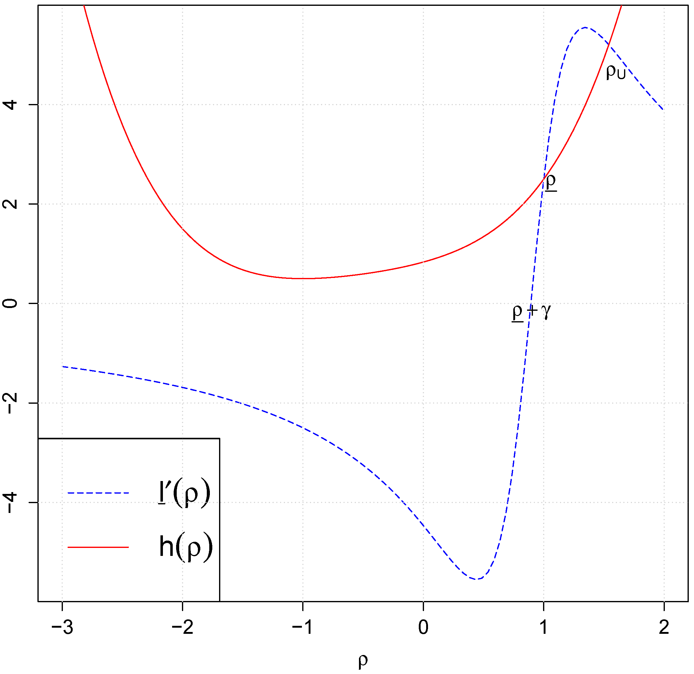
11] noted such behaviour of ρ's marginal posterior in simulations, but did not discuss much on how to specify the boundary points. In Proposition 4, we provide a data dependent way to specify
and
, which is necessary for model comparison to avoid Bartlett's paradox. First note that the probability limit of
is
where
Proposition 4. If are the true set of exogenous regressors used to generate ,
under Assumption 1 and 2, asymptotically the marginal posterior of ρ in Equation (13) will have more than one stationary points satisfying : 3
stationary points when T is odd and 2 when T is even, regardless of the true value of ρ. The local posterior mode, which is a consistent point estimator, is the stationary point nearest to the MLE satisfying asymptotically, which the other stationary point(s) do not satisfy. can be specified as the stationary point on the right of the posterior mode. When T is odd, can be specified as the stationary point on the left of the posterior mode; when T is even, could be chosen as a function of N such that is sufficiently small.
4 Choosing the boundary points as in Proposition 4 can ensure the marginal posterior of ρ to be proper and its support to contain the true value of ρ asymptotically.
and
are different from the boundary points in the constrained maximization in Dhaene and Jochmans [
8], who only considered parameter estimation. The interval of our boundary points is wider than theirs, since we want to preserve the bell-shaped part of the posterior density curve for model comparison. Another point to note is that when the true exogenous regressors are included, the local posterior mode will exist regardless of the true value of ρ (even if it is 1) due to Assumption 2.2 (e). Next we investigate the consequences when we can not include the true regressors.
3. Motivations and Methods to Compare Different Model Specifications
In empirical applications, researchers are often faced with many possible regressors suggested by different economic theories to be included into Equation (
1). Different models are defined by the inclusion of different combinations of the exogenous regressors and by whether or not the lagged dependent variable is present. Proposition 5 below implies there is no guarantee that the posterior mode in Equation (
13) is a consistent estimator if some true regressors are excluded from the model.
Proposition 5. The posterior mode in Equation (13) is a consistent estimator for ρ if and only if we have eitherorwhereHere represents the regressors in the true model and X denotes the regressors we actually include in our candidate model, while is the true value of ρ.
The values of
and
depend on how the true regressors and the included regressors are related, apart from the values of β and
. For
to be satisfied, it suffices that the true regressors
are a subset of
X.
5 When some true regressors are excluded, the model will suffer omitted variable bias unless Equation (
21) holds. Given Assumption 1 and 2, one example for Equation (
21) to hold could be that all the true regressors are covariance stationary and they have no serial correlation; the included regressors have zero correlation with the true regressors; moreover,
. For this restrictive case, it will be possible to estimate ρ consistently without any true regressors included.
6To avoid inconsistent estimation due to model misspecification, one could include all the potential regressors into the model. For finite sample, however, that could inflate the posterior variances for the coefficients of the true regressors if too many irrelevant regressors are included. The simulation studies in
Section 5 reveal that while including all the regressors does not influence the estimation of ρ in comparison to other consistent approaches, it leads to substantially high RMSE when estimating β. Hence appropriate procedures for model selection are desirable. In a Bayesian framework, one can evaluate different model specifications, denoted by
below, by their posterior model probabilities, which can be calculated as
where
denotes the regressors included under
and
is the marginal likelihood, obtained by integrating out ρ in Equation (
13) or (
43) in
Appendix C.
K is the number of all potential exogenous regressors. The total number of models is therefore
.
is the prior model probability of model
j. For finite samples, Ley and Steel [
15] showed that the choice of prior model probability will affect the posterior results to a large extent when the number of potential regressors is large compared to the sample size. In what follows, we focus on the asymptotic behaviour of posterior model probabilities and assume all the models are equally possible a priori. The posterior model probability
will hence only depend on
.
4. Consistency in Model Selection
In this section, we discuss the situations when the posterior model probability of the true model will tend to 1 as N tends to infinity. We will also analyze whether Bayesian information criterion (BIC) based on biased MLE is consistent in model selection.
For static panel models when the true value of ρ is zero and the lagged dependent variable is not included as a regressor, the analysis of Bayes factors is similar to that of Fernandez
et al. [
16]. In our context, we can ensure model selection consistency by setting
η as a function of
N with
for
. As for BIC, it is consistent in model selection for static panel models.
Let us now consider the case when our candidate model (
) contains
and
.
is compared to either
, which has
but no
, or
, which has
and
.
denotes the exogenous regressors included under model
for
, which satisfy Assumption 2.1 and 2.2.
can be the same or different from
, while
is different from
. The Bayes factors respectively are:
where
denotes the number of columns in
;
,
and
in
defined in Equation (
14) are calculated by replacing
with
in Equations (15) to (17) for
, which multiplied by
have the following probability limits under Assumption 1 and 2 with
and
:
stands for the Nickell MLE bias of ρ under
. We can see the MLE bias results from two sources: the incidental parameter part (
) and the model misspecification part (
). Proposition 4 shows that when the model is correctly specified, the local posterior mode is a consistent estimator for ρ. In the simulation studies in
Section 5 we find that when some combination of the wrong exogenous regressors are included, the marginal posterior density of ρ can be either monotonically increasing or is U-shaped depending on the value of
T and does not have a local maximum. When we find such a wrong model, we will assign 0 as its posterior model probability and will not estimate the model. In Proposition 6 and 7 below, we consider the cases when the local maximum exists for
in Equation (
18) and show the sufficient conditions under which the Bayes factors in Equations (
25) and (
26) can lead to the selection of the true model asymptotically. Denote
as the local maximum of
in
with
.
Proposition 6. When is the true model, i.e., and is the set of true regressors to generate Y, as N increases, in Equation (25) will tend to infinity if the following holds, When is the true model, i.e., is the set of true regressors and ,
as N increases, in Equation (25) will tend to 0 if either of the following is satisfied: If Equation (21) is true under ,
Equation (32) will hold. (b) Equation (20) is true under .
In this case, the left hand side of Equation (32) is equal to 0. Proposition 7. When is the true model and is the misspecified model, as N increases, in Equation (26) will tend to 0 if either of the following holds: If Equation (21) is true under ,
Equation (33) will hold. (b) Equation (20) is true under .
In this case, the left hand side of Equation (33) is equal to 0. Since both Equations (
20) and (
21) imply that the local posterior mode in Equation (
13) is a consistent estimator for ρ, from Proposition 6 and 7, we can see that if the posterior mode is consistent under the misspecified model, the misspecified model will not be chosen by the Bayes factor (model selection will be consistent). In
Appendix D, we show that
is positive over ℝ when
T is an even number. This implies
is an increasing function over ℝ. Also note that
. Hence
for
and it is possible for Equation (
31) to be violated when
T is even and
is a negative number. As shown in the last paragraph in
Appendix E, though Equation (
31) could be violated for the extreme case of
and
, fortunately, apart from this extreme case, violation of Equation (
31) could only occur when
for
T being an even number greater than 2, which may not be relevant for most economic applications with
.
Note that Equation (
32) is the special case of Equation (
33) with
. When the posterior mode is not consistent under the misspecified model, it is difficult to state under what circumstances Equation (
33) is or is not satisfied since
generally does not have closed form. By construction,
is a local minimum for the left of Equation (
33). In our simulation studies in
Section 5, we calculate Equation (
32) or (
33) under different settings when model selection errors based on Bayes factors occur. We cannot find a single occurrence of either Equation (
32) or (
33) being violated except the cases when Equation (
20) is true, that is, when the candidate model nests the true model. It appears that the left hand sides of Equation (
33) could be interpreted as how close the candidate model is to nest the true model. Note that with real data, it is difficult to check Equation (
20), but one can assess whether Equation (
33) is violated by replacing
with
and supplanting
and
by their consistent estimates e.g., those from the model including all the potential regressors.
Proposition 8 below shows when the BIC based on the biased MLE is consistent in model selection. BIC for the model with and without the lagged dependent variable is defined respectively below,
where
a,
b and
c are defined respectively in Equations (15), (16) and (17) with
, and
k is the number of exogenous regressors included. The model with smaller BIC value will be preferred.
Proposition 8. For the comparison of the two models in Equation (25), when is the true model, BIC will be consistent if the following is satisfied However, if Equation (20) is true under ,
the left of Equation (36) will be greater than 0 and BIC will be inconsistent. When is the true model, BIC will be consistent in model selection if the following condition is met: If is the same as and the probability limit of is equal to 0, the left of Equation (37) will be 0 and BIC will be inconsistent. For the comparison of the two models in Equation (26), when is the true model, BIC will be consistent in model selection if the following holds Conditions (
36), (
37) and (
38) are just the sufficient but not necessary conditions for BIC to be consistent in model selection since BIC has a penalty term against over-parameterization (the last term in Equations (
34) and (35)). Note that
and
from Equations (
27) and (28), where
γ is the Nickell bias. The violation of Equations (
36) and (
37) is related to the hypothesis test,
. When
(
) and
, the probability of making type I errors based on classical test statistics, such as Wald or likelihood ratio (LR), will be 1 and BIC will choose
asymptotically with the left hand side of Equation (
36) being
; when
and
, the probability of making type II errors will be 1 asymptotically and BIC will choose
even if
with the left hand side of Equation (
37) being
. When incidental parameters are present, Cox and Reid [
17] suggest using the likelihood conditional on the MLE of the orthogonalized incidental parameters to construct LR statistics. In practice, if we find
is close to 0 or the estimated Nickell bias, we should be cautious to use BIC for model selection. For Equation (
38), as shown in
Appendix G, if
is the true model and
nests
, the left hand side of Equation (
38) will be less than or equal to 0 asymptotically depending on whether
is less than or equal to
. Though Equation (
38) is violated when
, BIC can still favour
since there are more parameters under
. However, if
, which could happen when
is highly correlated with all the potential regressors, BIC will choose the wrong model
asymptotically, as shown in
Section 5.3. Given the SSR interpretation of
a in Equation (15) (with
), the practical implication of this result is that if BIC chooses the model with all the regressors included, which always has smaller
for finite sample comparing to other models, we should be cautious with such choice in the application.


