Article

Selection Criteria in Regime Switching Conditional Volatility Models

Aix-Marseille University (Aix Marseille School of Economics), CNRS & EHESS, Marseille, 13002, France
Econometrics 2015, 3(2), 289-316; https://doi.org/10.3390/econometrics3020289
Submission received: 13 January 2015 / Revised: 26 March 2015 / Accepted: 28 April 2015 / Published: 11 May 2015

Abstract

:
A large number of nonlinear conditional heteroskedastic models have been proposed in the literature. Model selection is crucial to any statistical data analysis. In this article, we investigate whether the most commonly used selection criteria lead to choice of the right specification in a regime switching framework. We focus on two types of models: the Logistic Smooth Transition GARCH and the Markov-Switching GARCH models. Simulation experiments reveal that information criteria and loss functions can lead to misspecification ; BIC sometimes indicates the wrong regime switching framework. Depending on the Data Generating Process used in the experiments, great care is needed when choosing a criterion.
JEL classifications:
C15; C22; C52

1. Introduction

Ever since Engle [1] developed the Autoregressive Conditional Heteroskedasticity (ARCH) models which provide a fruitful framework to analyze volatility and financial time series, this has been a major research focus in financial econometrics. Bollerslev [2] subsequently proposed Generalized Autoregressive Conditional Heteroskedasticity (GARCH) models, where volatility is a linear function of past volatility and squared residual past shocks. These models are of the form ϵ t = η t h t where h t is a positive process (volatility) and η t an identically and independently distributed random variable with zero mean and unit variance. Although GARCH models are attractive, copious empirical evidence in the econometric literature argues against their suitability. For example, these models do not adequately fit the data over a long period of time. Lamoureux and Lastrapes [3] show that if structural changes are not considered, upward GARCH estimates of persistence in variance may be biased. Moreover, while the squares of a GARCH(1,1) process follow the dynamics of an ARMA process with an autocorrelation function (ACF) which goes to zero very fast, the sample ACFs of the squares tend to stabilize around a positive value for larger lags. This is known as long range dependence in volatility. To circumvent these problems, practitioners can use other types of model, such as regime switching models. Several regime switching behaviors exist: in this paper we focus on regime switches driven by a hidden Markov Chain and regime switches driven by a transition function. Markov Switching GARCH (MS-GARCH) models belong to the first class. They have stochastic regime switches, and volatility can therefore take different forms depending on probabilities. Asymmetric GARCH models belong to the second class. The volatility has deterministic regime switches: it depends on a transition variable through a particular transition function, for example, a logistic smooth function which gives the Logistic Smooth Transition GARCH (LST-GARCH) model.
Practitioners studying empirical data need to choose a specific model to estimate conditional volatility. The wrong model will lead to incorrect interpretation of data. For example,selecting the wrong type of regime switching could cause a structural change to be confused with asymmetry. A well-known citation from Box [4] says that “Models, of course, are never true but fortunately it is only necessary that they be useful”. Thus, models are just an approximation of the true Data Generating Process (DGP). The challenge for data analysts is to select the best model, the one closest to the DGP. All the inferences and evaluations of real life data depend on accurate specifications yielding good in-sample forecasting results and more accurate interpretation of the economic world. This is known as goodness of fit. In practice, a set of plausible models is selected and narrowed down according to one of a number of criteria. The most popular are Information Criteria (IC), loss functions, and the R 2 from a regression. In time series analysis, IC and in-sample forecasts evaluated with loss functions are very often used. In contrast with out-sample forecasts, where in a lot of cases simpler models provide better results, in-sample forecasts should be better when the closest model is estimated.
In this article, we seek to identify whether certain criteria are more likely to lead to a good choice of regime switching type. To do so, we perform Monte Carlo experiments. We simulate data according to DGPs. We focus on two models: MS-GARCH and LST-GARCH. The estimation of LST-GACRH has been widely discussed in the literature; methods proposed include Quasi Maximum Likelihood (QML) estimation ([5,6]), Generalized Method of Moments ([7]) and Bayesian estimation ([8,9]). All these methods have advantages and drawbacks. We focus on the QML method here, since it is very commonly used in empirical applications. To our knowledge, the consistency and the asymptotic normality of LST-GARCH QML estimation has not been established yet1. There appear to be no findings on MS-GARCH models to date, nor on the asymptotic distribution of the Maximum Likelihood (ML) estimation. For example, Augustyniak [12] conducts an experiment which shows that Gray’s method does not generate consistent estimates for the path-dependent MS-GARCH model. These models suffer from a lack of theoretical grounding, and our aim here is to investigate the consequences on goodness-of-fit. Our experimental task is to estimate the data generated, using a wide variety of specifications. Finally, we apply various selection criteria to these estimations to see which model is chosen by the criteria. This method was employed in recent studies to highlight pitfalls in smooth transition models ([11]).
Our results raise interesting questions, revealing that selection criteria lead to misspecification in some cases. Does this mean that the criteria are not suitable for regime switching conditional volatility models? Probably not: we argue that if these criteria lead the choice of the wrong specification it is more because these regime switching models are difficult to estimate using the QML estimation, especially when the regimes are poorly identified in MS-GARCH models.
The remainder of this article is organized as follow out as follows. In Section 2, we briefly explain the different types of models and the selection criteria we explore. We present our simulation experiment framework in Section 3. Section 4 presents the results and the discussion. Section 5 contains concluding remarks.

2. Theory: Models and Selection Criteria

2.1. Models

In this section we describe the three classes of GARCH-type models that interest us here, explaining why we focus on these models. First, we describe the class of univariate GARCH models. Secondly, we present some asymmetric GARCH-type models: the LST-GARCH of Hagerud [6] and Gonzalez-Rivera [13], the Glosten-Jagannathan-Runkle (GJR) GARCH and the Exponential GARCH (EGARCH). Then, MS-GARCH-type models are introduced.

2.1.1. Univariate GARCH Model

The univariate GARCH model was introduced by Bollerslev [2] and many other followed. The GARCH model is a benchmark in volatility modeling since it can capture the main stylized facts of a financial time series that exhibit time-varying volatility clustering. A process ( ϵ t ) is called a GARCH(p,q) process if for t = 1 , , T , with T the sample size and
E ( ϵ t | ϵ s , s < t ) = 0 , t = 1 , , T
ϵ t = η t h t , η t I I D ( 0 , 1 )
with η t an identically and independent distributed random variable with zero mean and unit variance and if there exist ω, α j , j = 1 , , q and β i , i = 1 , , p such that
h t = V a r ( ϵ t | ϵ u , u < t ) = ω + j = 1 q α j ϵ t j 2 + i = 1 p β i h t i
GARCH-type models are generally estimated with the Gaussian Quasi Maximum Likelihood (QML) method. A QML estimation of the vector parameters θ 0 = ( ω 0 , α 01 , , α 0 q , β 01 , , β 0 p ) is defined as any solution θ ^ Q M L of
θ ^ Q M L = a r g m a x L = n 1 t = 1 T t
with
t = 1 2 log 2 π 1 2 log h t 1 2 ϵ t 2 h t
Gaussian QML estimation assumes that ϵ t are normally distributed. However, if this assumption is not verified, θ ^ Q M L is still consistent but can be inefficient, as shown in [14] and [15].

2.1.2. Asymmetric Volatility Models

This kind of model belongs to the class of “asymmetric” or “leverage” volatility models. They were introduced in response to empirical evidence that the increase in volatility is larger when returns are negative than when they are positive2. This characteristic is known as the “leverage-effect”. These models can be seen as regime switching GARCH models. They have different specifications according to the sign of the past shocks. We consider in this article three different asymmetric GARCH-type models: the LST-GARCH [6], the GJR-GARCH [20] and the EGARCH [21]. A process ( ϵ t ) is called an LST-GARCH(p,q) process if there exist ω, α 1 j , α 2 j , j = 1 , , q , β i , i = 1 , , p , and γ such that
h t = ω + j = 1 q [ α 1 j + α 2 j F ( ϵ t j ) ] ϵ t j 2 + i = 1 p β i h t i
where
F ( ϵ t j ) = ( 1 + e x p ( γ ϵ t j ) ) 1 1 2
with γ, the so-called transition parameter. The LST-GARCH process can be seen as a generalization of the well-known GJR-GARCH. A process ( ϵ t ) is called a GJR-GARCH(p,q) process if there exist ω, α 1 j , α 2 j , j = 1 , , q and β i , i = 1 , , p such that
h t = ω + j = 1 q [ α 1 j + α 2 j 𝟙 ( ϵ t 1 > 0 ) ] ϵ t j 2 + i = 1 p β i h t i
where 𝟙 ( . ) is the indicator function. When γ + , the logistic function becomes a double step function like the indicator function in the GJR-GARCH. In terms of regime, because the logistic function is continuous, Gonzalez-Rivera [13] talks about a “continuum” of regimes where the probability of regime switching is one. However, the term “regimes” does not have the same meaning as in the MS-GARCH models. Conditions for a stationary positive process are given in Hagerud [6] and Gonzalez-Rivera [13]. There is empirical evidence of how difficult it is to estimate the transition parameter3. We will therefore try to determine whether this inefficient selection criteria. Finally, we consider the popular EGARCH model by Nelson [21]. A process ( ϵ t ) is called an EGARCH(p,q) process if there exist ω, α 1 j , α 2 j , j = 1 , , q and β i , i = 1 , , p
log ( h t ) = ω + j = 1 q g j ( η t j ) + i = 1 p β i log ( h t i )
where
g j ( η t j ) = α 1 j η t j + α 2 j ( | η t j | + E | η t | )
The function g j depends on the magnitude and sign of η t . This makes it possible to respond asymmetrically to positive and negative values of the error term. As with the GARCH model, estimation is performed by maximizing the log-likelihood function given by L = t = 1 T t with t represented by Equation (5) assuming the normality of the error term.

2.1.3. MS-GARCH Models

These models give rise to a conditional mixture distribution. They allow time-varying skewness contrary to the traditional GARCH-type models: asymmetry exists in the conditional return distribution but this asymmetry is time-varying ([22]). Their main difference from the previous model is the following, for t = 1 , , T :
r t = ϵ t
with
ϵ t = η t h t ( Δ t )
and η t an identically and independently distributed random variable with zero mean and unit variance. Δ t is a variable which indicates the state of the world at time t . We will focus on MS-GARCH processes: Δ t follows a Markov chain with finite state spaces S = 1 , . . . , k , and a transition matrix P. However, other models exist where transition probabilities have a different definition. In contrast to the LST-GARCH process, the probability of switching from one regime to another is no longer equal to one but depends on the transition matrix P, given by
P = p 11 p k 1 p 1 k p k k
with p i j = p ( Δ t = j | Δ t 1 = i ) the probability of being in state j at time t, given of being in state i at time t 1 . In this sense, this type of regime switch is endogenous. A process ( ϵ t ) is called a MS(k)-GARCH(p,q) process if
ϵ t = η t h t ( Δ t ) , η t I I D ( 0 , 1 )
and there exist ω ( Δ t ) , α i ( Δ t ) , i = 1 , , q , β l ( Δ t ) , l = 1 , , p and j = 1 , , k such that
h t ( Δ t ) = ω ( Δ t ) + i = 1 q α i ( Δ t ) ϵ t q 2 + l = 1 p β l ( Δ t ) h t l
This model cannot be estimated by QML. The calculation of the likelihood function for a sample of T observations is infeasible because it requires the integration of k T possible regime paths ([23] and [24]). To circumvent the path dependence problem, Gray [5] introduces an MS-GARCH model under the hypothesis that the conditional variance at any regime depends on the expectation of previous conditional variance. He proposes to replace h t 1 by the conditional variance of the error term ϵ t 1 given the information up to t 2 . Klaassen [25] enlarges the information set to t 1 by conditioning the expectation of previous conditional variances on all available observations and also on the current regime:
h t ( Δ t ) = ω ( Δ t ) + α ( Δ t ) ϵ t 1 2 + β ( Δ t ) i = 1 k p ( Δ t 1 = i | Ω t 1 , Δ t = j ) h i , t 1
with j = 1 , . . . k and Ω t is the information set of the process (i.e., the return history up to date t 1 ). The model of Klaassen is the second model of interest. The model of Haas et al. [26] contrasts with this approach where each specific conditional variance depends only on its own lag,
h t ( Δ t ) = ω ( Δ t ) + α ( Δ t ) ϵ t 1 2 + β ( Δ t ) h t 1 ( Δ t )
This model can be rewriten in matrix form:
h t = ω + α ϵ t 1 2 + β h t 1
where ω = [ ω 1 , ω 2 , . . . , ω j ] , α = [ α 1 , α 2 , . . . , α j ] and β = d i a g ( β 1 , β 2 , . . . , β j ) . h t is thus a vector of k × 1 components. In this specification, every regime can be represented as an A R C H ( ) , which is the direct generalization of the single-regime GARCH model. This specification permits practitioners to interpret the coefficients in the same way as in the single regime framework. These two MS-GARCH models4 can easily be estimated by Maximum Likelihood (ML) estimation following the work of Hamilton [28]. An ML estimation of θ 0 , with the vector parameters θ 0 = ( ω 0 , α 0 , β 0 ) to be estimated is defined as any solution of θ ^ M L of
θ ^ M L = a r g m a x L = t = 1 T log f ( ϵ t | Ω t 1 )
where f ( ϵ t | Ω t 1 ) is the conditional density of ϵ t given the process up to time t. This density is the sum of conditional regime densities weighted by the conditional regime probabilities P r ( Δ t = j | Ω t 1 , θ ) . These probabilities are obtained by using the recursive scheme proposed by [29]. Moreover, in-sample forecasts of volatility are computed using these predicted probabilities:
h ^ t = j = 1 k P r ( Δ t = j | Ω t 1 , θ ^ M L ) h t , j
Finally, an assumption on conditional regime densities has to be made. In this paper, we investigate a case where the conditional regime densities follow a Gaussian density. As noted by [25,30,31], if regimes are not normal but leptokurtic, the use of within-regime normality affects identification of the regime process. It implies, for example, that ML estimation based on Gaussian components does not provide a consistent estimator. Hereafter, for convenience, we call the processes MSG-GARCH-K and MSG-GARCH-H respectively, for Klaassen [25] and Haas et al. [26], assuming Gaussian conditional regime densities. Moreover, we call the processes MST-GARCH-K and MST-GARCH-H respectively, for Klaassen [25] and Haas et al. [26], assuming Student conditional regime densities.

2.2. Selection Criteria: Information Criteria and Loss Functions

In empirical analysis, model selection is based on different methods. A statistical specification test comparing LST-GARCH and MS-GARCH processes does not exist yet5. The remaining way of choosing a specification for a model is to use the selection criteria. We focus on IC and in-sample forecasts. In contrast to hypothesis testing, they can be used to compare two models which have different specifications and which are not necessarily nested. According to Akaike [33], a model should be selected on the basis of good results when it is used for prediction. He proposed the well-known AIC to evaluate models in terms of Kullback-Leibler (KL) information ([34]),
A I C = 2 m 2 log ( L ( θ ^ | X ) )
where L ( θ ^ | X ) represents the value of the likelihood function in θ ^ , the vector of the estimated parameters, given the observed data and m the number of parameters. In general linear models, AIC tends not to perform well in small samples but the criterion tends to select the right model in large samples as shown in [35]. BIC has a similar form,
B I C = m log ( T ) 2 log ( L ( θ ^ | X ) )
with T the sample size. AIC imposes less of a penalty on the number of parameters than does BIC. In contrast to AIC, BIC is reputed to perform poorly in small samples in the context of general linear models.
In-sample forecasting can also be used to compare the real volatility with the predicted volatility. Loss functions measure the difference, and the model with the lowest loss is selected. However, volatility is a latent variable: in practice we do not observe real volatility, so we use proxies to compute it. Hansen and Lunde [36] show that the sufficient condition for a loss function to be robust is that L ( σ 2 , h ) ( σ 2 ) 2 does not depend on h, with σ ^ 2 the proxy and h the predicted volatility. Patton [37] derives necessary sufficient conditions. Moreover, he provides a new class of loss functions that guarantee the consistency of the ranking (asymptotically) when the unbiased volatility proxy is used instead of true volatility. The following class requires the assumption that the volatility proxy is unbiased. Loss functions are defined as
R ( σ ^ , h , b ) = 1 ( b + 1 ) ( b + 2 ) ( σ ^ 2 b + 4 h b + 2 ) 1 b + 1 ( h b + 1 ( σ ^ 2 h ) ) b { 1 , 2 } σ ^ 2 l o g σ ^ 2 h ( σ ^ 2 h ) b = 1 σ ^ 2 h l o g σ ^ 2 h 1 b = 2
with b a scalar parameter. In this article, we focus on three loss functions: Mean Squared Error (MSE), Quasi Likelihood (QLIKE) and Mean Absolute Error (MAE). MSE and QLIKE are special cases of Equation (16) when b = 0 and b = 2 respectively whereas MAE is not a robust loss function. For t = 1 , , T they are each equal to
M S E : L ( σ ^ t , h t ) = 1 T t = 1 T ( σ ^ t 2 h t ) 2
Q L I K E : L ( σ ^ , h t ) = 1 T i = 1 T ( σ t ^ 2 h t l o g σ t ^ 2 h t 1 )
M A E : L ( σ ^ , h t ) = 1 T t = 1 T | σ ^ 2 h t |
One important difference between MSE and QLIKE is that the former treats positive and negative errors equally, while the latter imposes a larger penalty when the forecast underestimates the realized volatility.

3. Design of the Experiments

The objective of our study was to perform Monte-Carlo experiments to see if the most commonly used information criteria and loss functions lead practitioners to choose the right specification in a conditional volatility regime switching framework. Since many practitioners use these models, it is important to assess the performance of the selection criteria, in order to guide professionals in their model selection process. This section gives details of the different experiments.

3.1. Common Design: Starting Values and Numerical Method

First, we present all the features of our overall experimental framework. In all the the experiments, data are first generated following a specific DGP described in great detail with more details below. Then, all the different models are estimated6. Finally, the selection criteria and loss functions presented in Section 2 are computed. According to the criteria, we report the percentage of selection for each specific model. Since we simulate our data, the real value of the volatility is known, but in order to come as close as possible to reality, squared errors are also used to compute the loss functions. DGPs are restricted to the LST-GARCH(1,1) and the MS(2)-GARCH(1,1) models. We focus on these models because there is some evidence in the literature that their estimation can be problematic: for example, the latent regime state estimation of MS-GARCH models. Our objective is therefore to show that these problems can lead to a deterministic regime switching type being chosen instead of a stochastic one, resulting in spurious interpretations. To interpret our results, we propose a working hypothesis that defines whether a selection criterion is efficient in this simulation framework:
Remark 1 From now on, we consider a selection criterion as strongly efficient if and only if it leads to the selection of the true DGP in at least 90 % of cases. Moreover, we consider a selection criterion as weakly efficient if and only if it leads to selection of the true DGP regardless of the assumption on the distribution of the error term in at least 90 % of cases.
The first part of our working hypothesis is very restrictive. In this case, we consider a selection criterion as efficient only if the entire true DGP is selected. The second part relaxes the misspecification on the error distribution. For example, if the true DGP is the MSG-GARCH-H and the selection criterion leads to selection of the MST-GARCH-H in 95% of cases, we conclude that it is only weakly efficient. Each simulation experiment is replicated 2000 times with a sample size7 T = 2000 . With the estimation framework described in the previous section, we face the well-known issue of selecting the starting values to initialize the local optimization procedure. For the likelihood function, we use traditional methods. The sample data variance is used to initialize the conditional variance and we employ ergodic probabilities to set the parameters governing the Markov Chain for MS-GARCH models, as recommended by [29]. To handle the issue of the initial parameter values, we use the true generating values when they are known. Otherwise, starting values for the parameters are selected from a grid of ten different random sets. We specify a plausible range for the parameters to avoid unusual sets. Thus, we draw the vectors θ ˜ g = ( ω 1 , α 1 , β 1 , ν ) , θ ˜ l s t = ( ω 1 , α 1 , α 2 , β 1 , γ , ν ) , θ ˜ g j r = ( ω 1 , α 1 , α 2 , β 1 , γ , ν ) , θ ˜ e g = ( ω 1 , α 1 , α 2 , β 1 , γ , ν ) and θ ˜ M S = ( ω 1 , ω 2 , α 1 , 1 , α 1 , 2 , β 1 , β 2 , p 11 , p 22 , ν ) which are respectively the vectors of starting values of the GARCH, LST-GARCH, GJR-GARCH, EGARCH and MS-GARCH models used in the estimation. All the parameters are drawn using a uniform distribution: ω j U ( 0 . 0001 ; 0 . 5 ) , α 1 U ( 0 . 1 ; 0 . 3 ) , α 2 U ( 0 . 15 ; 0 . 15 ) , α 1 , j U ( 0 . 1 ; 0 . 3 ) , β j U ( 0 . 4 ; 0 . 9 ) , γ U ( 0 ; 5 ) and p j j U ( 0 ; 1 ) . Parameter ν is null when data are estimated under the normality assumption. In the Student case, ν also follows a uniform distribution such that ν U ( 2 . 1 ; 10 ) . For each set of starting values, we check the positivity and the stationarity of the process. If the constraints are not verified, we draw another set of starting values. The set which gives the highest likelihood is selected to start the estimation procedure, which is based on the fmincon MATLAB routine. The options remain the same for all estimations. We also check for optimization convergence by checking the output structure of the fmincon function. If the procedure does not converge, we try another set of starting values until optimization convergence is achieved.

3.2. Experiment 1: Simulation of MS-GARCH-K Processes

The purpose of the first experiment is to generate data following an MS-GARCH-K process. As mentioned in Section 2.1.3, there are two different approaches to an MS-GARCH process. This experiment focuses on the traditional approach, the one adopted in [25]. Data are generated following Equation (12). The simulation procedure is the following. We start by generating the random error vector { η t } and the regime process vector { Δ t } for t = 1 , , T . The random errors are drawn randomly from a Gaussian distribution8. The regime process variable follows a Markov chain with finite state space S = { 1 , 2 } and a 2 × 2 transition probability matrix P = p 11 p 21 p 12 p 22 . Next, we construct9 h 1 ( Δ 0 ) = ω ( Δ 0 ) + α ( Δ 0 ) ϵ 0 2 + β ( Δ 0 ) h 0 and ϵ 1 = η 1 h 1 . Finally, we compute recursively the sequence { h 2 , ϵ 2 , , h T , ϵ T } where h t = ω ( Δ t ) + α ( Δ t ) ϵ t 1 2 + β ( Δ t ) h t 1 and ϵ t = η t h t . In this approach h T depends on the entire history of regimes up to T. The variance specification of Klaassen [25] is reasonable since, as in the standard GARCH model, past shocks and past variances affect today’s variances. However, it is not in keeping with the initial aim of GARCH models, which is the representation of a high order ARCH process. In this first experiment, we use four different transition matrices and two sets of GARCH parameters. For the first three cases, we have ω = 0 . 001 0 . 05 , α 1 = 0 . 2 0 . 1 and β = 0 . 4 0 . 85 . We focus on three different transition matrices P 1 = 0 . 1 0 . 9 0 . 9 0 . 1 , P 2 = 0.5 0.5 0.5 0.5 and P 3 = 0.9 0.1 0.1 0.9 . In this framework, the long-run (i.e., unconditional) probabilities10 are equal for each process. However, the regime persistence δ 11 differs. Matrix P 1 represents the case where regime switches occur often (anti-persistence), while the second matrix, P 2 , represents the case where the probability of remaining in the same regime is equal to the probability of switching regime (short memory behavior). The last case, matrix P 3 (long memory behavior) represents persistent regimes. In a fourth case, we use a different specification for both the Markov chain and the GARCH parameters. The first regime occurs very few times, with high unconditional variance. The second regime is the most common regime, with low unconditional variance : ω = 0.1 0.05 , α 1 = 0.4 0.1 and β = 0.9 0.4 with P 4 = 0.1 0.1 0.9 0.9 . The long-run probability of being in the first regime is equal to 0.1 while the long-run probability of being in the second regime is 0.9. In this setup the first regime is highly non-stationary, and can be seen as a jumps regime: at a time t a jump occurs (regime 1), but since this regime is not persistent, we go back rapidly to the normal regime (regime 2). However, the overall process is in good keeping with conditions described in [26]. We focus mainly on transition matrices because they are the source of stochastic regime switches. The probability of switching tends to one when switching rates increase. In this case, the selection criteria could fail to identify the true nature of the model.

3.3. Experiment 2: Simulation of MS-GARCH-H Processes

The second approach is introduced by [26] and defined by Equation (14). The simulation procedure differs from the first experiment in its second and the third steps. As before, we start by generating the random error vector { η t } and the regime process vector { Δ t } for t = 1 , , T . The random errors are drawn randomly from both a Gaussian distribution and a Student distribution with a degree of freedom ν = 5 . The state variable Δ t follows a Markov chain with finite state space S = { 1 , 2 } and a 2 × 2 transition probability matrix P = p 11 p 21 p 12 p 22 . In the second step, we construct h 1 = ω + α ϵ 0 2 + β h 0 , h 1 ( Δ 1 ) and ϵ 1 = η 1 h 1 ( Δ 1 ) 12. In the third step, we compute recursively the sequence { h 2 ( Δ 2 ) , ϵ 2 ( Δ 2 ) , , h T ( Δ T ) , ϵ T ( Δ T ) } where h t ( Δ t ) = ω ( Δ t ) + α ( Δ t ) ϵ t 1 2 + β ( Δ t ) h t 1 ( Δ t ) . All specific conditional variances need to be computed at each period: h t = ω + α ϵ t 1 2 + β h t 1 . Note that if the variable Δ t switches, the conditional variance differs instantaneously. Then, the error term is generated: ϵ t = η t h t ( Δ t ) . The set of parameters are the same as in the first experiment, so that results can be compared. However β = 0.4 0 0 0.85 for P 1 , P 2 and P 3 and β = 0.9 0 0 0.4 for P 4 due to notation.

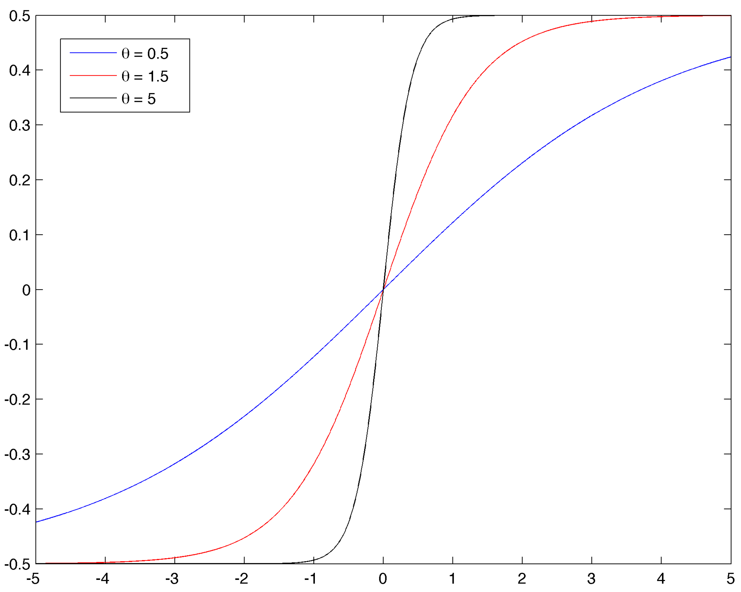
3.4. Experiment 3: Simulation of LST-GARCH Processes

In this third experiment, the underlying process is an LST-GARCH. The DGP of such a model is more trivial since there is no latent process. It is described by Equation (6) for p = q = 1 . To simulate this process, we start by drawing η t from a Gaussian distribution. Then, we compute recursively h t and ϵ t 13. As in the first experiment, we estimate the data with all the models. We focus on three different sets of parameters. γ is the parameter of interest since it governs the transition function. If the transition parameter is large, the transition function becomes steep and we can see it as a “two regimes” model, as shown by Figure 1. The sets of parameters are ω = 0 . 05 , α 1 = 0 . 3 , α 2 = 0 . 55 , β = 0 . 3 and γ = { 0.5 , 1.5 , 5 } .
Figure 1. Logistic functions with different γ.
Econometrics 03 00289 g001

4. Results and Discussion
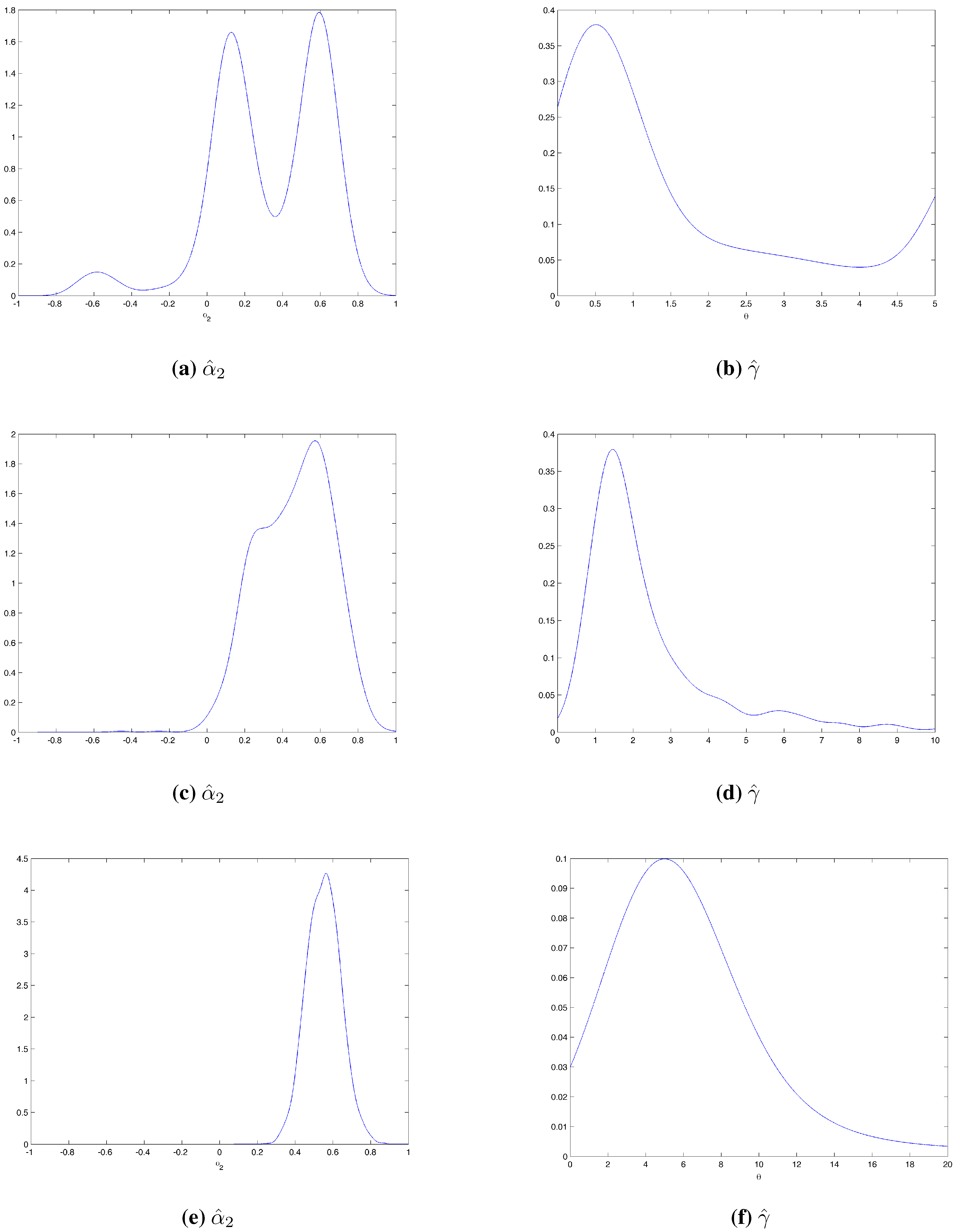
4.1. Results

Table 1 sums up the results. It shows whether or not the selection criteria are weakly efficient as defined in remark 1. Table 2 to Table 12 present in detail the results of the three Monte-Carlo experiments described in Section 3. The choice percentage is given per selection criterion. For example, in Table 2, the GARCH model is selected in first position by AIC in 16.6% of cases. Our results show that when regimes are difficult to identify (i.e., many regime switches or one regime occurring very few times) and data are generated as per Klaassen, information criteria and loss functions do not find always the true DGP. Thus, practitioners could make the wrong choices in these cases. Moreover, squared residuals should not be used as a proxy of volatility ; we encourage practitioners to use different proxies, like realized volatility. In addition, the results show that information criteria perform poorly when LST-GARCH is the generating process.

4.1.1. Experiment 1

In this first experiment, the DGPs are MS-GARCH-K path-dependent with Gaussian innovations. With the first set of parameters, the transition probabilities are high: there are a lot of regime switches. The results of the selection process are presented in Table 1 row 1 and in Table 2. In this case, none of the criteria are strongly or weakly efficient as defined by our working hypothesis. However, if we sum the results for both MSG-GARCH-K and MST-GARCH-K, loss functions select the right model at a rate of 71.3% for MSE, 86.1% for QLIKE and 83.7% for MAE. They come close to the weakly efficient point. Loss functions computed with ϵ t 2 often select the wrong model whatever the process used to simulate the data, and thus are not efficient with this volatility proxy. What stands out is the poor performance of information criteria. AIC does not enable us to choose between MSG-GARCH-K and the univariate GARCH-T model, while BIC is weakly inefficient, leading to choice of a GARCH model in 98.9% of cases.
Table 1. Summary of the results of experiments 1 and 2. A cross means that the criterion is weakly efficient as defined in remark 1.
DGPMSE( h t )QLIKE( h t )MAE( h t )MSE( ϵ t 2 )QLIKE( ϵ t 2 )MAE( ϵ t 2 )AICBIC
Experiment 1 and 2 with Gaussian innovations
P 1 MS-K
MS-Hxxx xx
P 2 MS-K
MS-Hxxx xx
P 3 MS-Kxxxxxxxx
MS-Hxxx xx
P 4 MS-K
MS-Hxxxxxxxx
Experiment 2
γ = 0.5 LST-G
γ = 1.5 LST-G
γ = 5 LST-G
Table 2. Results of experiment 1 with MSG-GARCH-K DGP when many switches occur. Data are generated with the transition matrix P 1 . The top row of the table gives the selection criteria. The left column gives the different models. The line in grey indicates the process which should be selected in first position by each criterion. Regime persistence and volatility persistence are respectively δ = 0.8 and λ = 0.9228 .
MSE( h t )QLIKE( h t )MAE( h t )MSE( ϵ t 2 )QLIKE( ϵ t 2 )MAE( ϵ t 2 )AICBIC
GARCH7.23.80.500016.667.8
GARCH-T4.22.10.500032.231.1
MSG-GARCH-H8.04.913.233.552.259.26.60
MST-GARCH-H0.40.60.695.32.30.30
MSG-GARCH-K30.746.154.349.134.234.027.10
MST-GARCH-K40.640.629.48.48.34.51.10
LST-GARCH1.10.90.10000.40
LST-GARCH-T1.30.200001.30
GJR0.70.40.10003.80.8
GJR-T0.70.30.10005.50.1
EGARCH3.10.10.40002.00.1
EGARCH-T2.000.80002.10
With the matrix P 2 (Table 1 row 3, Table 3), there are fewer regime switches. AIC and BIC lead to do the wrong choices at a respective rate of 57.9% and 94.6%. This frequency is a little bit lower than where there are many regime switches. The second model chosen by AIC is the MSG-GARCH-H. AIC leads to the right choice of regime switching behavior in 82.5% of cases. The rate of regime switching errors decreases, since we less often select the GARCH model. In contrast, BIC still selects the GARCH Student specification at a rate of 82.3%. As in the previous case, the in-sample forecasts selection method improves the frequency of good choices. However, these selection criteria need to be more than weakly efficient. Loss functions computed with ϵ t 2 return good results when data are simulated with MS-GARCH-K. The results are better than in the previous experiment: the percentage of good selection increases for all loss functions. For example, MSE leads to 49.1% good selection with the transition matrix P 1 , increasing to 74.6% with P 2 .
Table 3. Results of experiment 1 with MS-GARCH-K DGP when probabilities of remaining are equal to probabilities of switching. Data are generated with the transition matrix P 2 . The top row of the table gives the selection criteria. The left column gives the different models. The line in grey indicates the process which should be selected in first position, by each criterion. Regime persistence and volatility persistence are respectively δ = 0 and λ = 0 . 9165 .
MSE( h t )QLIKE( h t )MAE( h t )MSE( ϵ t 2 )QLIKE( ϵ t 2 )MAE( ϵ t 2 )AICBIC
GARCH0.50.1000001.8
GARCH-T0.200.10008.282.3
MSG-GARCH-H24.017.323.813.321.619.321.45.2
MST-GARCH-H9.37.05.45.61.71.58.40.2
MSG-GARCH-K36.146.149.574.672.774.442.15.4
MST-GARCH-K21.929.419.66.54.04.812.70.1
LST-GARCH00.1000000
LST-GARCH-T0.4000000.20
GJR0.20000000.1
GJR-T0000003.30.5
EGARCH6.101.600000.1
EGARCH-T1.3000003.74.3
This improvement is accentuated when data are generated with persistent regimes. Let us consider MSG-GARCH-K and MST-GARCH-K together. In this case, all the decision criteria are weakly efficient (Table 1 row 5, Table 4). Specification errors is reduced to below 10 % . All the selection criteria are efficient in this case. However, if these two models are compared, the Student version may be selected even though the data are generated with Gaussian errors.
In the fourth case, the two variances are totally different. Selection criteria lead to the choice of a misspecified model in this case (Row 7, Table 1 and Table 5). For example, BIC selects the simple GARCH model at a rate of 69.4% and the GARCH-T with at rate of 28.8%. The MSG-GARCH-K is never selected by this criterion. Loss functions do not work any better. Although MSE selects, in first position, the right model, the rate is very low (22.2%). No model is clearly selected in first position. Under the definition in remark 1, they are all inefficient and fail to recognize the true regime switching behavior.
Table 4. Results of experiment 1 with MSG-GARCH-K DGP when regime-specific variances are persistent. Data are generated with the transition matrix P 3 . The top row of the table gives the selection criteria. The left column gives the different models. The line in grey indicates the process which should be selected in first position, by each criterion. Regime persistence and volatility persistence are respectively δ = 0.8 and λ = 0.9147 .
MSE( h t )QLIKE( h t )MAE( h t )MSE( ϵ t 2 )QLIKE( ϵ t 2 )MAE( ϵ t 2 )AICBIC
GARCH00000000
GARCH-T00000000
MSG-GARCH-H5.15.54.41.9 0.16.47.9
MST-GARCH-H3.24.31.30.10.101.70.2
MSG-GARCH-K48.843.164.785.793.690.172.288.8
MST-GARCH-K42.947.129.612.25.99.819.73.1
LST-GARCH00000000
LST-GARCH-T00000000
GJR00000000
GJR-T00000000
EGARCH0000.10000
EGARCH-T00000000
Table 5. Results of experiment 1 with MS-GARCH-K DGP when the first regime has a high variance which occurs very few times. Data are generated with the transition matrix P 4 . The top row of the table gives the selection criteria. The left column gives the different models. The line in grey indicates the process which should be selected in first position, by each criterion. Regime persistence and volatility persistence are respectively δ = 0 and λ = 0.8888 .
MSE( h t )QLIKE( h t )MAE( h t )MSE( ϵ t 2 )QLIKE( ϵ t 2 )MAE( ϵ t 2 )AICBIC
GARCH8.45.75.700021.969.4
GARCH-T7.35.55.90.100.143.828.8
MSG-GARCH-H13.815.514.534.725.827.25.30
MST-GARCH-H10.010.36.027.616.820.20.20
MSG-GARCH-K22.234.241.730.051.945.35.00
MST-GARCH-K14.919.716.77.45.27.00.50
LST-GARCH3.81.71.20000.20
LST-GARCH-T4.83.31.80.20.201.00
GJR2.31.11.500.106.91.4
GJR-T2.22.32.10009.90.1
EGARCH5.10.51.10001.90.2
EGARCH-T5.20.21.8000.13.40.1

4.1.2. Experiment 2

In this second experiment, the DGP is now an MS-GARCH as per of Haas et al. There is a significant contrast with the previous experiment. In the first case (row 2 of Table 1 and Table 6), information criteria are all strongly efficient as defined by remark 1. As highlighted by Table 6, AIC and BIC select the MSG-GARCH-H model at a rate of 93.6% and 99.4% respectively. Loss functions computed with the true volatility h t return a selection rate of over 50%. The MSG-GARCH-H is always selected in first position. If the percentage selection of the MSG-GARCH-H and the MST-GARCH-H are summed, loss functions are weakly efficient. The MST-GARCH-H model provides a very good fit with data generated by an MSG-GARCH-H model.
Table 6. Results of experiment 2 with MS-GARCH-H DGP when many switches occur. Data are generated with the transition matrix P 1 . The top row of the table gives the selection criteria. The left column gives the different models. The line in grey indicates the process which should be selected in first position, by each criterion. Regime persistence and volatility persistence are respectively δ = 0.8 and λ = 0.9228 .
MSE( h t )QLIKE( h t )MAE( h t )MSE( ϵ t 2 )QLIKE( ϵ t 2 )MAE( ϵ t 2 )AICBIC
GARCH00000000
GARCH-T00000000
MSG-GARCH-H52.346.967.812.249.87.893.699.4
MST-GARCH-H45.745.930.27.67.62.36.35.0
MSG-GARCH-K0.93.91.165.830.670.80.10.1
MST-GARCH-K13.30.912.012.019.100
LST-GARCH00000000
LST-GARCH-T00000000
GJR00000000
GJR-T00000000
EGARCH0.10000000
EGARCH-T00000000
With matrix P 2 (Table 1 row 4, Table 7), there are again no selection problems. The rate of good selection improves in all cases. As previously, information criteria and loss functions computed with the true volatility are largely weakly efficient. However, poor performance is observed with the loss functions computed with the squared residuals. In these cases, there are errors in choosing between the two MS-GARCH-type processes.
When the regimes are persistent, the results are similar to those of the previous experiment where the DGP was the MSG-GARCH-K (Table 1 row 6, Table 8). All the criteria are efficient except when computed with volatility proxy, which leads to the selection of the MSG-GARCH-K model.
Finally, in the last special case (Table 1 row 8, Table 9), the results are very interesting; the MSG-GARCH-H is selected with a strong majority by loss functions. If we add the number of selections of the MST-GARCH-H, the selection criteria based on in-sample forecasts are weakly efficient. Information criteria seem to select the true DGP. AIC is near the strongly efficient point (89.9% of correct selection). BIC selects the MSG-GARCH-H at a rate of 74.9%. However, it also selects the GARCH-T model in 21.8 % of replications. The poor performance of squared residuals as a proxy of volatility is again evident.
Table 7. Results of experiment 2 with MS-GARCH-H DGP when probabilities of remaining are equal to probabilities of switching. Data are generated with the transition matrix P 2 . The top row of the table gives the selection criteria. The left column gives the different models. The line in grey indicates the process which should be selected in first position, by each criterion. Regime persistence and volatility persistence are respectively δ = 0 and λ = 0.9165 .
MSE( h t )QLIKE( h t )MAE( h t )MSE( ϵ t 2 )QLIKE( ϵ t 2 )MAE( ϵ t 2 )AICBIC
GARCH00000000
GARCH-T00000000
MSG-GARCH-H57.954.676.834.257.239.094.999.2
MST-GARCH-H41.139.519.15.13.22.85.00.6
MSG-GARCH-K0.73.23.753.436.854.10.10.2
MST-GARCH-K0.22.70.47.33.34.100
LST-GARCH00000000
LST-GARCH-T00000000
GJR00000000
GJR-T00000000
EGARCH00000000
EGARCH-T00000000
Table 8. Results of experiment 2 with MSG-GARCH-H DGP when regime specific variances are persistent. Data are generated with the transition matrix P 3 . The top row of the table gives the selection criteria. The left column gives the different models. The line in grey indicates the process which should be selected in first position, by each criterion. Regime persistence and volatility persistence are respectively δ = 0.8 and λ = 0.9147 .
MSE( h t )QLIKE( h t )MAE( h t )MSE( ϵ t 2 )QLIKE( ϵ t 2 )MAE( ϵ t 2 )AICBIC
GARCH00000000
GARCH-T00000000
MSG-GARCH-H59.964.679.248.719.135.997.999.8
MST-GARCH-H39.532.819.113.12.87.52.00
MSG-GARCH-K0.61.81.731.273.050.00.10.2
MST-GARCH-K00.106.95.16.600
LST-GARCH0000.10000
LST-GARCH-T00000000
GJR00000000
GJR-T00000000
EGARCH00000000
EGARCH-T00000000
Table 9. Results of experiment 2 with MSG-GARCH-H DGP when the first regime has a high variance which occurs very few times. Data are generated with the transition matrix P 4 . The top row of the table gives the selection criteria. The left column gives the different models. The line in grey indicates the process which should be selected in first position by each criterion. Regime persistence and volatility persistence are respectively δ = 0 and λ = 0.8888 .
MSE( h t )QLIKE( h t )MAE( h t )MSE( ϵ t 2 )QLIKE( ϵ t 2 )MAE( ϵ t 2 )AICBIC
GARCH00000000
GARCH-T0000001.321.8
MSG-GARCH-H88.282.087.273.083.664.289.974.9
MST-GARCH-H8.88.75.313.53.85.91.80.1
MSG-GARCH-K3.09.37.513.212.529.76.33.0
MST-GARCH-K0.1000.20.10.200
LST-GARCH00000000
LST-GARCH-T00000000
GJR00000000
GJR-T0000000.60.1
EGARCH0000.10000
EGARCH-T0000000.10.1

4.1.3. Experiment 3

We report the results of this experiment in the last three rows of Table 1, Table 10, Table 11, and Table 12. None of the selection criteria are efficient when γ is low. However, in this case, loss functions computed with the true volatility yield the best results: roughly 40% correct selection for MSE, QLIKE and MAE loss functions, regardless of the assumption on distribution. The volatility proxies are clearly inefficient and, importantly, they lead to selection of an MS-GARCH-type process in about 80% of cases. Information Criteria also lead the wrong choice of model. BIC is strongly inefficient since it selects a GARCH(1,1) model at a rate of 96.3%. The non-linear effect affecting conditional volatility is not recognized in this case.
When γ = 1.5 , the logistic function is less smooth (red line in Figure 1). Results are presented in Table 11. Loss functions computed with the true volatility have a good selection rate roughly 80%. Thus, they are close to the weakly efficient point. However, they still perform poorly when we use ϵ t 2 . The information criteria again fail to select the true DGP, selecting the LST-GARCH model in only 23.4% of cases for AIC and 1.3% for BIC. All the other univariate GARCH-type models are selected in preference to the LST-GARCH, especially the GJR.
The number of GJR selections with both AIC and BIC is shown to increase when γ increases (Table 12). There is also a large non-negligible number of selections of the EGARCH model. Moreover, the performance of MSE and MAE loss functions computed with h t tends to be worse when γ = 5 . Despite this, errors are not made on the asymmetric effect presents in the conditional volatility. The selection criteria never select Markov switching models, except for the volatility proxy loss functions. This experiment shows that when γ is not large enough, the asymmetric behavior of the conditional volatility may not be detected. Moreover, when γ is too large, the GJR model is a good choice because it avoids the estimation issues encountered with the LST-GARCH.
Table 10. Selection results of experiment 3 with a smooth logistic function. Data are generated with a LST-GARCH model with γ = 0.5 . The top row of the table gives the selection criteria. The left column gives the different models. The line in grey indicates the process which should be selected in first position, by each criterion. The volatility persistence is λ = 0.825 .
MSE( h t )QLIKE( h t )MAE( h t )MSE( ϵ t 2 )QLIKE( ϵ t 2 )MAE( ϵ t 2 )AICBIC
GARCH4.39.96.90.10056.296.3
GARCH-T4.08.86.40.300.22.60.2
MSG-GARCH-H1.82.24.029.621.913.71.30
MST-GARCH-H2.82.55.21.53.525.000
MSG-GARCH-K1.11.92.341.861.345.240
MST-GARCH-K4.37.56.53.93.45.100
LST-GARCH30.932.327.37.32.51.93.50
LST-GARCH-T16.711.118.86.04.61.90.10
GJR14.510.09.91.41.90.926.53.3
GJR-T14.813.511.41.100.31.00
EGARCH2.20.20.83.90.83.08.00.2
EGARCH-T2.60.10.53.10.12.80.40
Table 11. Selection results of experiment 3 with a smooth logistic function. Data are generated with a LST-GARCH model with γ = 1.5 . The top row of the table gives the selection criteria. The left column gives the different models. The line in grey indicates the process which should be selected in first position, by each criterion. Volatility persistence is λ = 0.825 .
MSE( h t )QLIKE( h t )MAE( h t )MSE( ϵ t 2 )QLIKE( ϵ t 2 )MAE( ϵ t 2 )AICBIC
GARCH0000.1007.434.8
GARCH-T0.10.40.10.2000.60
MSG-GARCH-H00.20.128.025.114.10.10
MST-GARCH-H00.10.10.61.923.900
MSG-GARCH-K0.10.2031.958.941.80.10
MST-GARCH-K0.10.403.24.04.200
LST-GARCH43.463.543.110.45.33.223.41.3
LST-GARCH-T33.019.834.58.02.31.82.00
GJR9.76.09.21.51.21.24641.3
GJR-T11.19.310.82.700.93.00.1
EGARCH1.40.71.35.91.24.716.322.5
EGARCH-T1.10.40.87.524.21.10
Table 12. Selection results of experiment 3 with a smooth logistic function. Data are generated with a LST-GARCH model with γ = 5 . The top row of the table gives the selection criteria. The left column gives the different models. The line in grey indicates the process which should be selected in first position, by each criterion. The volatility persistence is λ = 0.825 .
MSE( h t )QLIKE( h t )MAE( h t )MSE( ϵ t 2 )QLIKE( ϵ t 2 )MAE( ϵ t 2 )AICBIC
GARCH0000.10000.1
GARCH-T00000000
MSG-GARCH-H00033.433.222.800
MST-GARCH-H0000.81.019.700
MSG-GARCH-K00030.047.337.000
MST-GARCH-K0004.45.43.900
LST-GARCH48.062.849.57.23.82.428.91.8
LST-GARCH-T19.626.026.38.88.46.31.30
GJR18.15.313.56.30.83.255.892.8
GJR-T14.35.910.78.40.14.53.10.3
EGARCH0000.405.710.95.0
EGARCH-T0000.200.200

4.2. Discussion

To summarize the results presented in Section 4.1, we point out three main selection issues. The first one is whether Student models can outperform Gaussian models for in-sample forecasts. The second is that information criteria perform poorly in some special cases. Finally, we find that squared standardized residuals are a bad proxy for volatility when making in-sample forecasts.
The first issue is interesting. Since the Student distribution tends to the Gaussian distribution when the degree of freedom tends to infinity, it is not surprising that the MST-GARCH can fit MSG-GARCH data well. Moreover, there is no problem with interpretation. Even when a misspecification error is made on the distribution, it does not impact regime switching behavior.
We propose two possible explanations for the poor results obtained with some selection criteria. First, when two processes are similar, the likelihood of model misspecification may be higher. The likelihood value is the principal component of information criteria. MS-GARCH processes with P 1 are anti-persistent since λ = 0 . 8 and the probabilities of switching are equal to 0.9. In asymmetric models, regime switches are deterministic and depend on a transition function. Thus, the equation for h t changes in each period and the probability of switching is equal to one. It is not surprising that the univariate model fits well with MS-GARCH processes with a transition matrix of the form of P 1 . As shown by Guegan and Rioublanc [38], MS-GARCH models with this type of persistence have a similar autocorrelation function to the GARCH process. Moreover, the loss functions work better for the simple reason that the number of parameters impact the information criteria.
A second possible explanation is that, in mixture models, when there is a very small class that is hard to identify or when two classes are very similar, estimation may be less efficient, as pointed out by [39]. This is observed from the results of Table 2, Table 5, Table 6, Table 9, Figure 2 and Figure 3. The four tables correspond to cases where the long-run probabilities are low for at least one regime. Figure 2 gives box plots for each parameter of MSG-GARCH models when the model estimate corresponds to the DGP. This figure highlights the poor estimation efficiency of MSG-GARCH-K parameters when the transition matrices are P 1 or P 4 . Estimations are around the DGP values for both MS-GARCH models, but the variance is higher with MSG-GARCH-K (Figure 2(a) and Figure 2(b)). Moreover, there are more extreme values in this latter process, particularly for the estimation of transition probabilities. With P 3 , estimation errors are less frequent. Figure 3 represents the non-parametric density estimation14 of the simulated conditional volatility processes f ^ ( h t ) (solid lines) and the estimated conditional volatility processes f ^ ( h ^ t ) (dash-dash lines), for one replication15 with f the probability density function. Figure 3 shows the differences between the non parametric density functions when we use P 1 and P 3 . They point to a large difference between the two MSG-GARCH models, which can be explained by the construction of the MSG-GARCH-K. Although the computation of past conditional variance depends only on the previous state, h t is dependent on all the previous regimes. In the MSG-GARCH-H, regime-specific variances are totally independent. That is why both simulated MSG-GARCH-H volatility processes exhibit bimodal densities (blue solid line). Moreover, f ^ ( h ^ t ) seems to fit well f ^ ( h t ) . With MS-GARCH-K processes, f ^ ( h t ) functions (red solid lines) also have two modes but they are less apparent and wider. This is probably due to path-dependence behavior. Although the approximation of Klaassen is attractive, it sometimes fails to adequately fit the overall volatility time series of the path-dependent MSG-GARCH-K model; we can see that f ^ ( h ^ t ) (red dash-dash line) does not exhibit the two modes when the regimes switch a lot (Figure 3(a)). Of course, these figures represent only one replication, but things are very similar for the others. All this illustrates why BIC does not choose the right model (results of Table 2, Table 3 and Table 7): if the regimes are not properly identified, the estimation will be less accurate and the value of the likelihood function lower. Thus, AIC and BIC have higher values and become inaccurate in selecting the model. The loss functions computed with the true volatility are not affected by the likelihood value and are more efficient than the information criteria.
Finally, the impact of using ϵ t 2 differs depending on the loss function and the DGP. For example, the frequency of good choices indicated by the QLIKE loss function decreases when regimes become more persistent and the DGP is the MSG-GARCH-H, whereas it increases when the DGP is the MSG-GARCH-K. However, this proxy works better than information criteria when data are simulated by MSG-GARCH-K. Other proxies which are unbiased and contain much more information should give better results, so we encourage practitioners to use them to estimate RS-GARCH models. Similar remarks are made in [36,37,40] regarding the selection of models using an out-sample forecasts approach. The authors cited above recommend the realized volatility for example.
Our two experiments yield three main findings: first, when data are simulated in the sense of Haas, information criteria are a powerful means of selecting the right model. Secondly, loss functions seem to work well when the DGP is MSG-GARCH-K. Finally, although ϵ t 2 is not a good proxy, it gives good results when data are generated in the sense of Klaassen. Our results also highlight the strong impact that estimation has on the efficiency of these criteria.
Figure 2. Box plots of MSG-GARCH parameter estimations. (a) MS-GARCH-K with P 1 ; (b) MS-GARCH-H with P 1 ; (c) MS-GARCH-K with P 2 ; (d) MS-GARCH-H with P 2 ; (e) MS-GARCH-K with P 3 ; (f) MS-GARCH-H with P 3 ; (g) MS-GARCH-K with P 4 ; (h) MS-GARCH-H with P 4 .
Econometrics 03 00289 g002
Figure 3. Non-parametric density estimation of the simulated and estimated conditional volatility for one replication in Experiment 1 and 2. (a) Transition matrix P 1 ; (b) Transition matrix P 3 .
Econometrics 03 00289 g003
With the third experiment, our framework reveals estimations of α 2 and γ to be very imprecise, as represented in Figure 4. This Figure gives the non-parametric density estimation16 of α 2 and γ for the three cases that we investigate. Figure 4(a) shows that α 2 is very poorly estimated when the transition parameter is low; although there is a mode around 0.55 , the true value of α 2 , a second mode appears around 0.1 . More surprisingly, there is a third mode around 0.55 , i.e., we sometimes estimate an opposite asymmetric effect. A plausible explanation is that when the transition parameter is low, the logistic function is substantially flatter. As a result, estimating the coefficient attached to the logistic function and transition parameter is harder. Figure 4(c) and Figure 4(e) show that estimation works better when γ increases. Figure 4(b), Figure 4(d) and Figure 4(f) give the non-parametric density estimations of γ. They highlight the well-stylized fact that QML is not an accurate means estimating of this parameter. Despite this estimation problem, regime selection is good; on average, the criteria select at least the right regime switching behavior: MS-GARCH models do not capture the continuum of regimes introduced by Gonzalez-Rivera [13]. However, the GJR model adequately fits the LST-GARCH process. As for using squared residuals as a proxy for volatility, we do not recommend this any more than in the previous experiment.
Figure 4. Non-parametric density estimation of α 2 and γ for the three sets of parameters. (a,b) correspond to the first set γ = 0 . 5 ; (c,d) correspond to the second set γ = 1 . 5 ; and (e,f) correspond to the third set γ = 5 .
Econometrics 03 00289 g004

5. Conclusions

This paper presents simulation results regarding the properties of model selection criteria in a regime switching conditional volatility framework. Such models are often difficult to estimate due to their complex forms, posing a number of challenges, MS-GARCH models need to estimate many parameters. ST-GARCH models need to estimate a transition parameter, which is complicated. For example, Chan and McAleer [41] investigate the finite sample properties of MLE for Smooth Transition Autoregressive models (STAR) with GARCH component models. They show that the variability of the threshold value depends on the magnitude of unconditional shocks for the Logistic STAR model. They also examine misspecification on the transition function. Moreover, estimation by QML is know to be very sensitive to starting values.
This article contributes to three strands of the literature. First, we show that it is rare to make an error in the selection of regime switching behavior. Selection criteria manage to distinguish well between stochastic and deterministic switches in most cases. However, Information Criteria could lead practitioners to make the wrong choice between stochastic and deterministic regime switches. Loss functions computed with true volatility are more suitable for this purpose. The second contribution of this work concerns the selection of models based on selection criteria such as AIC, BIC or in-sample forecast performance. Through statistical analysis, we provide empirical evidence that results obtained using these selection criteria are directly impacted by estimation performance. Proper estimation of these models is important, and although regime switching GARCH models provide good indicators to explain the financial crisis17, selection needs to be made with great care. Estimation methods other than QML are available, like Bayesian or GMM estimations. However, with MS-GARCH models, ML is the one most commonly used in empirical work. Finally, we examine in-sample forecasts and show that the noisy proxy of squared returns is, in a lot of cases, not a good choice when selecting a volatility model.
In the first experiment, data are simulated following MSG-GARCH-K models with many transition matrices. Results show that BIC could lead to a majority selection of GARCH and LST-GARCH models when the regimes are not persistent or one of them occurs too often. In the same way, AIC selects MSG-GARCH-H. Loss functions improve model selection accuracy when computed with simulated volatility. Like many other authors, we find that squared errors are a very imprecise proxy for true volatility and these selection criteria do not lead to good results. In the third experiment, the underlying processes are LST-GARCH with different transition parameters. We show that the selection process is difficult when the transition parameter is not large enough or when it is too large. The GJR model may be a good candidate for such model estimations.
Our findings here reflect the complex nature of regime switching GARCH models, implying that practitioners need to perform careful before using this type of model.

Acknowledgments

I thank Anne Peguin-Feissolle and Emmanuel Flachaire for many valuable comments. Thanks also to Marjorie Sweetko for English language editing. Finally, I would like to thank Bilel Sanhaji and Gilles De Truchis who were always ready to help me. I am greatly indebted to participants for comments received at the CEF 2013 in Vancouver BC, the 13th OxMetrics User Conference in Aarhus and the 1st IAAE meeting in London. Finally, I would like to thank both reviewers for their insightful comments on the paper, as these comments led to an improvement of the work. Thanks also to Lu Liao, assistant editor of Econometrics, for the submission procedure which was a nice experience.

Conflicts of Interest

The author declares no conflict of interest.

References

  1. R.F. Engle. “Autoregressive Conditional Heteroscedasticity with Estimates of the Variance of United Kingdom Inflation.” Econometrica 50 (1982): 987–1007. [Google Scholar]
  2. T. Bollerslev. “Generalized autoregressive conditional heteroskedasticity.” J. Econom. 31 (1986): 307–327. [Google Scholar] [CrossRef]
  3. C.G. Lamoureux, and W.D. Lastrapes. “Persistence in Variance, Structural Change, and the GARCH Model.” J. Bus. Econ. Stat. 8 (1990): 225–34. [Google Scholar]
  4. G.E.P. Box. “Robustness in the strategy of scientific model building.” In Robustness in Statistics. Edited by R. L. Launer and G. N. Wilkinson. New York, NY, USA: Academic Press, 1978, pp. 201–236. [Google Scholar]
  5. S.F. Gray. “Modeling the conditional distribution of interest rates as a regime-switching process.” J. Financ. Econ. 42 (1996): 27–62. [Google Scholar] [CrossRef]
  6. G.E. Hagerud. “A Smooth Transition ARCH Model for Asset Returns.” In Working Paper Series in Economics and Finance 162. Sweden, Stockholm: Stockholm School of Economics, 1997. [Google Scholar]
  7. C. Francq, and J.M. Zakoïan. “Deriving the autocovariances of powers of Markov-switching GARCH models, with applications to statistical inference.” Comput. Stat. Data Anal. 52 (2008): 3027–3046. [Google Scholar] [CrossRef]
  8. L. Bauwens, A. Preminger, and J.V.K. Rombouts. “Theory and inference for a Markov switching GARCH model.” Econom. J. 13 (2010): 218–244. [Google Scholar] [CrossRef]
  9. M. Lubrano. “Smooth Transition Garch Models: A Baysian Perspective.” In Discussion Papers (REL—Recherches Economiques de Louvain) 2001032. Louvain, Belgium: Institut de Recherches Economiques et Sociales (IRES), Université Catholique de Louvain, 2001. [Google Scholar]
  10. F. Chan, M. McAleer, and M.C. Medeiros. “Structure and asymptotic theory for nonlinear models with GARCH errors.” EconomiA, 2015. [Google Scholar] [CrossRef]
  11. N. Maugeri. “Some Pitfalls in Smooth Transition Models Estimation: A Monte Carlo Study.” Comput. Econ. 44 (2014): 339–378. [Google Scholar] [CrossRef]
  12. M. Augustyniak. “Maximum likelihood estimation of the Markov-switching GARCH model.” Comput. Stat. Data Anal. 76 (2014): 61–75. [Google Scholar] [CrossRef]
  13. G. Gonzalez-Rivera. “Smooth-Transition GARCH Models.” Stud. Nonlinear Dyn. Econom. 3 (1998): 1–20. [Google Scholar]
  14. I. Berkes, and L. Horvàth. “The efficiency of the estimators of the parameters in GARCH processes.” Ann. Statist. 32 (2004): 633–655. [Google Scholar]
  15. C. Francq, and J.M. Zakoïan. “On Efficient Inference in GARCH Processes.” In Dependence in Probability and Statistics. Edited by P. Bertail, P. Soulier and P. Doukhan. New York, NY, USA: Springer, 2006, Volume 187, Lecture Notes in Statistics; pp. 305–327. [Google Scholar]
  16. F. Black. “Studies of stock price volatility changes.” In Proceedings of the 1976 Meetings of the American Statistical Association, Business and Economics Statistics Section, Boston, MA, USA, 23–26 August, 1976; pp. 177–181.
  17. Z. Ding, C.W. Granger, and R.F. Engle. “A long memory property of stock market returns and a new model.” J. Empir. Financ. 1 (1993): 83–106. [Google Scholar] [CrossRef]
  18. F.P. Hans, and D.V. Dijk. “Forecasting stock market volatility using (nonlinear) GARCH models.” J. Forecast. 15 (1996): 229–235. [Google Scholar]
  19. G.F. Loudon, W.H. Watt, and P.K. Yadav. “An empirical analysis of alternative parametric ARCH models.” J. Appl. Econom. 15 (2000): 117–136. [Google Scholar] [CrossRef]
  20. L.R. Glosten, R. Jagannathan, and D.E. Runkle. “On the Relation between the Expected Value and the Volatility of the Nominal Excess Return on Stocks.” J. Financ. 48 (1993): 1779–1801. [Google Scholar] [CrossRef]
  21. D.B. Nelson. “Conditional Heteroskedasticity in Asset Returns: A New Approach.” Econometrica 59 (1991): 347–370. [Google Scholar] [CrossRef]
  22. M. Rockinger, and E. Jondeau. “Entropy densities with an application to autoregressive conditional skewness and kurtosis.” J. Econom. 106 (2002): 119–142. [Google Scholar] [CrossRef]
  23. J.D. Hamilton, and R. Susmel. “Autoregressive conditional heteroskedasticity and changes in regime.” J. Econom. 64 (1994): 307–333. [Google Scholar] [CrossRef]
  24. J. Cai. “A Markov Model of Switching-Regime ARCH.” J. Bus. Econ. Stat. 12 (1994): 309–316. [Google Scholar]
  25. F. Klaassen. “Improving GARCH volatility forecasts with regime-switching GARCH.” Empir. Econ. 27 (2002): 363–394. [Google Scholar] [CrossRef]
  26. M. Haas, S. Mittnik, and M.S. Paolella. “A New Approach to Markov-Switching GARCH Models.” J. Financ. Econom. 2 (2004): 493–530. [Google Scholar] [CrossRef]
  27. G.M. Gallo, and E. Otranto. “Forecasting Realized Volatility with Changing Average Volatility Levels.” Int. J. Forecast., 2015. forthcoming. [Google Scholar]
  28. J.D. Hamilton. “A New Approach to the Economic Analysis of Nonstationary Time Series and the Business Cycle.” Econometrica 57 (1989): 357–384. [Google Scholar] [CrossRef]
  29. J.D. Hamilton. “Nonlinearities and the Macroeconomic Effects of Oil Prices.” Macroecon. Dyn. 15 (2011): 364–378. [Google Scholar] [CrossRef]
  30. D. Ardia. “Bayesian estimation of a Markov-switching threshold asymmetric GARCH model with Student-t innovations.” Econom. J. 12 (2009): 105–126. [Google Scholar] [CrossRef]
  31. M. Haas, S. Mittnik, and M.S. Paolella. “Asymmetric multivariate normal mixture GARCH.” Comput. Stat. Data Anal. 53 (2009): 2129–2154. [Google Scholar]
  32. L. Hu, and Y. Shin. “Optimal Test for Markov Switching GARCH Models.” Stud. Nonlinear Dyn. Econom. 12 (2008): 3. [Google Scholar] [CrossRef]
  33. H. Akaike. “A New Look at the Statistical Model Identification.” In Selected Papers of Hirotugu Akaike. Edited by E. Parzen, K. Tanabe and G. Kitagawa. Springer Series in Statistics; New York, NY, USA: Springer, 1998, pp. 215–222. [Google Scholar]
  34. S. Kullback, and R.A. Leibler. “On Information and Sufficiency.” Ann. Math. Stat. 22 (1951): 79–86. [Google Scholar] [CrossRef]
  35. C.M. Hurvich, and C.L. Tsai. “Regression and Time Series Model Selection in Small Samples.” Biometrika 76 (1989): 297–307. [Google Scholar] [CrossRef]
  36. P.R. Hansen, and A. Lunde. “Consistent ranking of volatility models.” J. Econom. 131 (2006): 97–121. [Google Scholar] [CrossRef]
  37. A.J. Patton. “Volatility forecast comparison using imperfect volatility proxies.” J. Econom. 160 (2011): 246–256. [Google Scholar] [CrossRef]
  38. D. Guegan, and S. Rioublanc. “Regime Switching Models: Real or Spurious Long Memory ? ” Available online: http://econpapers.repec.org/paper/haljournl/halshs-00189208.htm (accessed on 13 January 2015).
  39. S. Frühwirth-Schnatter. Finite Mixture and Markov Switching Models. Springer Series in Statistics; New York, NY, USA: Springer, 2006. [Google Scholar]
  40. S. Laurent, J.V. Rombouts, and F. Violente. “Consistent ranking of multivariate volatility models.” In CORE Discussion Papers 2009002. Louvain, Belgium: Université Catholique de Louvain, Center for Operations Research and Econometrics (CORE), 2009. [Google Scholar]
  41. F. Chan, and M. McAleer. “Maximum likelihood estimation of STAR and STAR-GARCH models: Theory and Monte Carlo evidence.” J. Appl. Econom. 17 (2002): 509–534. [Google Scholar] [CrossRef]
  42. C. Brunetti, C. Scotti, R.S. Mariano, and A.H. Tan. “Markov switching GARCH models of currency turmoil in Southeast Asia.” Emerg. Mark. Rev. 9 (2008): 104–128. [Google Scholar] [CrossRef]
  43. K.L. Chang. “Do macroeconomic variables have regime-dependent effects on stock return dynamics? Evidence from the Markov regime switching model.” Econ. Modell. 26 (2009): 1283–1299. [Google Scholar] [CrossRef]
  • 1.Some empirical studies have shown that the QML estimation of smooth transition models can cause problems in interpretation. See Chan et al. [10] and Novella [11].
  • 2.See [16,17,18,19].
  • 3.See [11] for example.
  • 4.There are a number of expansions of these two MS-GARCH processes. For example, Gallo and Otrento [27] introduce asymmetric effects in each regime variance.
  • 5.Hu and Shin [32] introduced a test procedure which tests the null hypothesis of a GARCH process against an MS-GARCH process.
  • 6.For each experiment, we estimate these models: GARCH, GARCH-T, LST-GARCH, LST-GARCH-T, GJR-GARCH, GJR-GARCH-T, EGARCH, AEGARCH-T, MSG(2)-GARCH-H, MSG(2)-GARCH-K, MST(2)-GARCH-H and MST(2)-GARCH-K.
  • 7.Results for T = 1000 are available on demand, results remain the same. We do not consider smaller sample size since in financial application, we used to study daily data.
  • 8.Klaassen [25] and Haas et al. [26], specifically address MS-GARCH models with Student-t distribution. While this case is interesting, we do not consider it in this paper, for the sake of simplicity.
  • 9.We set ϵ 0 = 0 , h 0 = 1 and Δ 0 = 1 . We generate 2000 more observations than required to minimize any starting bias.
  • 10.The probabilities of being in regime i = 1 , 2 . The long-run probability of the first regime: π 1 is equal to π 1 = 1 p 22 2 p 11 p 22 .
  • 11.δ is computed as follows: δ = p 11 + p 22 1 .
  • 12.We set ϵ 0 = 0 , h ( Δ 0 ) 0 = 1 and Δ 0 = 1 . We generate 2000 more observations than required, to minimize any starting bias.
  • 13.We generate 2000 more observations than required to minimize any starting bias.
  • 14.Estimation computed with Gaussian kernel and Silverman’s rule of thumb.
  • 15.Figure 3(a) is related to the 40th replication of the first and the second experiments with matrix P 1 , BIC selects the right specification when data are simulated with MSG-GARCH-H but it selects the GARCH model for data simulated with MS-GARCHG-K. Figure 3(b) is related to the 66th replication of the first and second experiments with P 3 where there is no selection problem.
  • 16.Estimation computed with Gaussian kernel and Silverman’s rule of thumb.
  • 17.Brunetti et al. [42] detect currency turmoil in southeast Asia with MS-GARCH models. Chang [43] uses Markov-Switching model to argue that macroeconomic variables have regime-dependent effects on stock return dynamics.

