Finding Starting-Values for the Estimation of Vector STAR Models

Abstract

This paper focuses on finding starting-values for the estimation of Vector STAR models. Based on a Monte Carlo study, different procedures are evaluated. Their performance is assessed with respect to model fit and computational effort. I employ (i) grid search algorithms and (ii) heuristic optimization procedures, namely differential evolution, threshold accepting, and simulated annealing. In the equation-by-equation starting-value search approach the procedures achieve equally good results. Unless the errors are cross-correlated, equation-by-equation search followed by a derivative-based algorithm can handle such an optimization problem sufficiently well. This result holds also for higher-dimensional Vector STAR models with a slight edge for heuristic methods. For more complex Vector STAR models which require a multivariate search approach, simulated annealing and differential evolution outperform threshold accepting and the grid search.

1. Introduction

Whatever the use of an econometric model, estimating its parameters as well as possible given the available information is of crucial importance. In this paper I focus on the estimation of Vector Smooth Transition Autoregressive (Vector STAR) models. Thereby, a non-linear optimization function originates which is commonly solved by a numerical, derivative-based algorithm. Yet, parameter estimation may come along with optimization difficulties. Problems due to flat or non-convex likelihood functions may arise. Hence, in empirical applications derivative-based optimization algorithms may either converge slowly to the global optimum or only to a local optimum which is not globally optimal (Maringer and Winker [1]).

Optimization problems of objective functions that are ill-behaved are well-known. One of the pioneering contributions is the work of Goffe et al. [2] who discuss optimization problems related to the use of conventional optimization techniques by proposing optimization heuristics as alternative estimation approach. Typically, regime-switching models are also afflicted with such optimization problems (Van Dijk et al. [3]).

As Teräsvirta and Yang [4] point out, the estimation outcome of Vector STAR models crucially relies on good starting-values. Initializing a derivative-based algorithm with starting-values close to the global optimum or at least close to a useful local optimum helps the algorithm to cover the remaining distance to the nearest optimum. Yet, in high-dimensional models trying several starting-values in order to get close to the global optimum may turn out to be extremely time-consuming or even not solvable in reasonable computing time. The present paper focuses on finding starting-values for the estimation of Vector STAR models to solve this complex problem. Different procedures for deriving starting-values are evaluated and their performance is assessed with respect to model fit and computational effort.

It is common to apply grid search methods for finding initial values. However, it has not been assessed whether other methods, namely heuristics, could perform better in generating starting-values. The inherent stochastics and (controlled) impairments of the objective function of heuristic optimization procedures may deliver advantages in terms of (i) the extent to which the surface area can be explored and (ii) the optimization outcome (higher likelihood). This is particularly important when equation-by-equation Non-linear Least Squares estimation is inefficient or not feasible at all and a system-wide Maximum Likelihood estimation is necessary. Recent contributions emphasize the benefit of employing alternative optimization approaches in non-linear models. These include heuristic methods, see for instance Baragona et al. [5], Battaglia and Protopapas [6], Chan and McAleer [7], El-Shagi [8], Maringer and Meyer [9], Wu and Chang [10], Yang et al. [11], and Baragona and Cucina [12]. The studies concentrate on parameter estimation in univariate or multivariate regime-switching models. The starting-value search and estimation of a Vector STAR model by means of heuristic methods has not been addressed in the literature so far. In principle, heuristics are qualified to be the final estimator, but they may converge slowly to the optimum. Before applying a heuristic algorithm to the whole modeling cycle of a non-linear Vector STAR model, one might initially focus on improving the starting-value search.

Based on a comprehensive Monte Carlo set-up, I address the starting-value search for the estimation of Vector STAR models. Different procedures for finding starting-values are evaluated and their performance is assessed with respect to model fit and computational effort based on simulated Data Generating Processes (DGPs) of Vector STAR models. I employ both grid search algorithms and—following the ideas of El-Shagi [8] and Gonzalez et al. [13]—three heuristic optimization procedures: differential evolution (DE), threshold accepting (TA), and simulated annealing (SA).

The main results of this study are as follows. For Vector STAR models with uncorrelated error terms equation-by-equation starting-value search procedures are preferable. In this case, all procedures perform equally well with a slight edge for the heuristic methods in higher-dimensional models. As soon as the Vector STAR model has cross-correlated error terms, multivariate starting-value search procedures, however, outperform equation-by-equation approaches. The comparison of different algorithms indicates that SA and DE improve parameter estimation. The latter result holds for Vector STAR models with a single transition function.

The paper is organized as follows. Section 2 introduces the Vector STAR model and its characteristics. The competing methods for finding starting-values are presented in Section 3. Section 4 describes the evaluation framework which is a comprehensive Monte Carlo study. The simulation results are presented in Section 5. Finally, Section 6 concludes.

2. The Vector STAR Model

The (logistic) Vector STAR model is a non-linear, multivariate regression model. It can capture different dynamic properties across regimes (asymmetric behavior), has a straightforward economic interpretation in different regimes and can handle smooth transitions from one regime into the other. It looks as follows:1

$${\mathbf{y}}_{\mathbf{t}}=\left\{\sum _{i=1}^m({\mathbb{G}}_{\mathit{t}}^{\mathit{i}-\mathbf{1}}-{\mathbb{G}}_{\mathit{t}}^{\mathit{i}}){\mathbf{F}}_{\mathbf{i}}^{\prime }\right\}{\mathbf{x}}_{\mathbf{t}}+{\epsilon }_{\mathit{t}}$$

(1)

where ${\mathbf{y}}_{\mathbf{t}}$ is a $k\times 1$ column vector and ${\mathbf{x}}_{\mathbf{t}}=({\mathbf{y}}_{\mathbf{t}-\mathbf{1}}^{\prime },\dots ,{\mathbf{y}}_{\mathbf{t}-\mathbf{p}}^{\prime },{\mathbf{d}}_{\mathbf{t}}^{\prime }){}^{\prime }$, where ${\mathbf{d}}_{\mathbf{t}}$ is a vector containing deterministic components. ${\mathbf{F}}_{\mathbf{i}}=({\mathbf{A}}_{\mathbf{i}\mathbf{1}}^{\prime },\dots ,{\mathbf{A}}_{\mathbf{ip}}^{\prime },{\Phi }_{\mathbf{i}}^{\prime }){}^{\prime }$, $i=1,\dots ,m$, includes coefficient matrices and is of dimension $(pk+q)\times k$. The error vector ${\epsilon }_{\mathit{t}}$ is assumed to be white noise with variance-covariance matrix Ω. ${\mathbb{G}}_{\mathbf{t}}^{\mathbf{i}}(.)$ is a diagonal matrix of transition functions such that different transition functions across equations can be modeled. Accordingly, ${\mathbb{G}}_{\mathbf{t}}^{\mathbf{i}}(.)$ reads:

$${\mathbb{G}}_{\mathbf{t}}^{\mathbf{i}}(.)=\text{diag}\left\{\mathbf{g}\left(s_{i1t}\right|{\gamma }_{i1},c_{i1}),\dots ,\mathbf{g}\left(s_{ikt}\right|{\gamma }_{ik},c_{ik})\right\}$$

(2)

for $i=1,\dots ,m-1$, where m determines the number of regimes in each equation and ${\mathbb{G}}_{\mathbf{t}}^{\mathbf{0}}={\mathbf{I}}_{\mathbf{k}}$, ${\mathbb{G}}_{\mathbf{t}}^{\mathbf{m}}=\mathbf{0}$. In the simulation exercise I stick to Vector STAR models with a single transition ($m=2$). The transition functions $\mathbf{g}(.)$ are assumed to be of logistic type which is monotonically increasing in the transition variable $s_{ijt}$, where $j=1,\dots ,k$, and bounded between zero and one:

$$\mathbf{g}\left(s_{ijt}\right|{\gamma }_{ij},c_{ij})={[1+\text{exp}(-{\gamma }_{ij}(s_{ijt}-c_{ij}))]}^{-1},{\gamma }_{ij}>0$$

(3)

The transition function depends on the transition speed (${\gamma }_{ij}$), the location parameter ($c_{ij}$) and the transition variable ($s_{ijt}$). Following Teräsvirta [14], in order to make γ a scale-free parameter, it is divided by the standard deviation of the transition variable when the parameters of the Vector STAR model are estimated.

The transition function which governs the transition from one regime to another is crucial in a Vector STAR model framework. In a multivariate framework, the number of transition functions, transition variable, transition speed and the location parameter may be different in each equation which is often also economically reasonable. There is also the special case where only one transition function governs the whole system, then, ${\mathbb{G}}_{\mathbf{t}}(.)=\mathbf{g}\left(s_t\right|\gamma ,c){\mathbf{I}}_{\mathbf{k}}$. In the simulation exercises, I will analyze different model specifications with respect to the number of transition functions and the parameter setting to evaluate the performance of competing starting-value search methods and their robustness across different specifications.

Amongst others, van Dijk et al. [3] discuss difficulties for estimating the slope parameter (${\gamma }_{ij}$) of a Vector STAR model when the latter is large. When the transition speed is high, the Vector STAR model converges to a switching regression model. Determining the curvature might be problematic since a low number of observations around the location parameter could make the estimation of the slope parameter rather inaccurate in small samples. Thus, relying on suitable starting-values for the transition speed becomes even more important. The slope parameter ${\gamma }_{ij}$ and thereby, the Vector STAR model can be redefined by

$${\gamma }_{ij}=\text{exp}\left({\nu }_{ij}\right)$$

(4)

where ${\nu }_{ij}$ is the parameter to be estimated. This methodological sophistication has not been applied in the literature so far and is clearly an improvement and a simplification over existing approaches for finding starting-values.2 The slope parameter ${\gamma }_{ij}$ in Equation (3) can then be replaced by the expression in Equation (4). In general, ${\gamma }_{ij}>0$ is an identifying restriction such that the codomain is restricted to be the set of positive real numbers. This implies that the previous redefinition is a bijective transformation. Redefining ${\gamma }_{ij}$ facilitates the construction of the grid because one can build an equidistant grid in the dimension of ${\nu }_{ij}$. Consequently, the search space for ${\gamma }_{ij}$ is automatically dense in the beginning and less so when it becomes large which is a sensible choice for estimating the Vector STAR model.

The estimation problem can be simplified by concentrating the likelihood function w.r.t. $\mathbf{F}$, as conditionally on known values of $\Gamma =\left[{\gamma }_{ij}\right]$, $\mathbf{C}=\left[c_{ij}\right]$ the model is linear (Leybourne et al. [15]. As a consequence for the starting-value search, the—then linear—model can be either estimated by equation-by-equation Ordinary Least Squares (OLS) or system-wide by Feasible Generalized Least Squares (FGLS). If the vector system share the same transition function, equation-by-equation OLS is not feasible and FGLS needs to be applied. Moreover, the latter estimation approach is efficient if the simultaneous equation model has zero restrictions in the lag structure and/or has cross-correlated error terms (Greene [16] (Chapter 14)).

Based on the derived initial values, the non-linear optimization is carried out either by an equation-by-equation Non-linear Least Squares (NLS) algorithm or a system-wide Maximum Likelihood (ML) approach based on derivative-based optimization algorithms. NLS minimizes equation-wise the residual sum of squares. The covariance matrix is estimated once at the end. Recall that initial values for the NLS estimation are obtained by OLS as described in the previous paragraph. In contrast to NLS, ML cannot be conducted equation-by-equation. Starting-values are obtained by the system estimation approach FGLS. ML does then also take the variance-covariance matrix (Ω) into account in the estimation by maximizing the loglikelihood.3 Whenever there are neither cross-correlations nor zero restrictions equation-by-equation NLS is efficient.

The estimation problem is bounded with respect to ${\gamma }_{ij}$ and $c_{ij}$ in order to constrain the parameter estimates to reasonable values. The constraints are being set to match the support of ${\gamma }_{ij}$ and $c_{ij}$, see the following Section 3 for more details.4 For a more detailed description of specification, estimation and evaluation of Vector STAR models see Teräsvirta and Yang [4] and for a survey on Vector Threshold and Vector Smooth Transition Autoregressive Models see Hubrich and Teräsvirta [17].

3. Starting-Value Search Methods

In the following I present the competing starting-value search methods. SubSection 3.1 presents the grid search methods—classical grid and grid with a zoom. Subsequently, SubSection 3.2 introduces the heuristic methods: threshold accepting, simulated annealing, and differential evolution.

Some general remarks regarding the search space of Γ and $\mathbf{C}$ are appropriate at this point. The search space of the location parameter $c_{ij}$ is defined to be a function of the transition speed: $c_{ij}=f\left({\gamma }_{ij}\right)$. The function works as follows: If γ is large, implying a low number of observations around the threshold, a truncated sample of the observations of the transition variable for the location parameter c is used. At most, the lower and upper 15% percentile are excluded which is also recommended by Andrews [18] and Caner and Hansen [19] for Threshold (V)AR models. If γ is small, the support of c is not restricted. In other words, 100% of the transition variable observations are used as support.

${\gamma }_{ij}$ is bounded between 0.1 and 30. It is necessary to constrain the parameter set as the Vector STAR model becomes unidentified otherwise. The transition function is practically constant if γ gets very small. A slope parameter equal to 30 is already close to an abruptly switching Threshold VAR model.

Recall that the slope parameter is redefined by $\gamma =\text{exp}\left(\nu \right)$ for facilitating the starting-value search. This yields the new set $\mathbf{N}=\left[{\nu }_{ij}\right]$. Consequently, the bounds are also redefined to $\mathbf{N}=\text{ln}(\Gamma )$.

3.1. Grid Search

3.1.1. Classical Grid

The classical grid search (GS) constructs a discrete grid based on the parameter space of $\mathbf{C}=\left[c_{ij}\right]$ and $\Gamma =\left[{\gamma }_{ij}\right]$, respectively $\mathbf{N}=\left[{\nu }_{ij}\right]$. For each fixed pair, thus each point in the grid, the (then linear) model is estimated and an objective value function is calculated. The value which optimizes the objective function is selected and its corresponding parameter values for ν and c yield the starting-values. In higher dimensional models a multidimensional grid emerges assuming an equation-specific transition function.

The parameter (search) space of $\mathbf{C}=\left[c_{ij}\right]$ is based on the actual realization of the transition variable depending on the current value of ${\gamma }_{ij}$ as described above. For the redefined parameter set of $\mathbf{N}=\left[{\nu }_{ij}\right]$, I use an equidistant search space with increments of 0.003 yielding a grid which is then dense for low values of γ and less so for steeper regions. The increments are chosen to match approximately the average number of likelihood evaluations of the heuristic starting-value search methods.

3.1.2. Grid with a Zoom

The number of grid points increases quickly with model dimension and number of transition functions. Hence, it is likely that the number of grid points are intractable to estimate in a reasonable computing time if a multivariate search approach is required. To circumvent the time-consuming grid search in higher dimensional models, Yang [20] suggests a grid with a zoom which builds new grids by using the best solution of the previous step as the center. The initial step is a grid with a rather moderate number of grid points in each dimension. In the implementation I use five, yielding 25 grid points for each pair, as recommended by Yang [20]. In the next step, the new grid is based on the neighboring points of the previously optimal solution. The zoom-in is discontinued when for all parameters ($\mathbf{N}$ and $\mathbf{C}$) the difference between the highest and smallest value building the new grid is smaller than a given value. 0.001 will be used in the implementation. Finer differences in parameters do not change the objective function value. The stepwise refinement and zoom-in have the ability to find a global optimum if the likelihood is centered around one optimum and thus, does not have many local optima. The grid with a zoom might, however, miss the global or a useful local optimum, if the surface area is not well-behaved.

The zoom-in with a moderate grid clearly leads to a lower number of likelihood evaluation in contrast to the classical grid and heuristic techniques. However, since the heuristic methods are equipped with a stopping criterion which may exit the algorithm earlier, they may have a lower amount as well (details can be found in the following SubSection 3.2).

To match the number of likelihood evaluations, one could also increase the number of grid points. Yet, we would then lose the time advantage of the grid with zoom. Moreover, increasing the number of grid points of the zoom-in may not necessarily result in superior outcomes because of the potential inability of this approach to find a global optimum of a non-smooth surface.5

3.2. Heuristic Optimization Algorithms

In the class of optimization heuristics, I focus on local search methods which iteratively search for a new solution in the neighborhood of the current solution by using a random mechanism. The central idea of the local search methods is to allow temporary uphill or downhill moves, i.e., a (controlled) impairment of the objective function value.6 This is done in order to escape local optima. The algorithms start off with a random guess such that they do not depend on subjective elements. In case of multiple local optima, heuristic methods may find better optima than traditional methods.

I assess the performance of different heuristic optimization algorithms in order to obtain a successful, fast and easily applicable modeling strategy. In general, heuristics can be divided into two categories: population based methods and trajectory methods. The starting-values search within a multivariate Vector STAR model relies on a continuous search space. Differential evolution (DE) which belongs to the class of population based methods might be preferable in this case (Gilli and Winker [21]). These kinds of methods update a set of solutions simultaneously. Additionally, I employ threshold accepting (TA) and simulated annealing (SA). They are trajectory methods that work on a single solution, i.e., these procedures alter the value of only one parameter in each iteration step. The heuristic methods are described in more detail in the next sections beginning with trajectory methods.7

3.2.1. Threshold Accepting

Algorithms 1 and 2 show pseudocodes for a minimization problem. In line 1 of Algorithm 1 the number of iterations I and restarts R as well as the threshold sequence T are initialized. The threshold sequence which is used for the acceptance decision gets linearly lowered to zero within 80% of the iterations. It is based on a data-driven threshold sequence which is endogenously generated from the sample (see Winker and Fang [22] for details).8 Line 2 shows the initialization of the (equation-specific) parameters of the transition speed and location parameter. The initial slope parameter (γ) of the transition function is drawn from an exponential distribution function with an expected value one ensuring a positive value. The initialized values of γ are transformed and the search procedure is based on $\nu =ln\left(\gamma \right)$. The initial location parameter (c) is drawn randomly from a uniform distribution covering a certain range of the transition variables’ actual realizations. As described above, c is a function of γ ensuring a feasible support of c based on the current value of γ. When updating the parameters, the slope and location parameter are forced to remain in predefined bounds. When γ (ν) or c do not lie in the interval, they are set equal to their predefined bounds: 0.1 (ln(0.1)) and 30 (ln(30)) and lowest/highest value of the feasible range of the transition variable, respectively. Based on the initial parametrization, an equation-by-equation OLS estimation or system FGLS estimation is performed. As can be seen in line 3 of Algorithm 1, an objective function—error variance or loglikelihood—is calculated to compare different parametrizations. This objective function value is stored.

After the initialization, the iterations start in line 4. The neighbor solution is computed in the next step, see line 5 in Algorithm 1. The following details can be found in Algorithm 2. A random draw determines whether the location or slope parameter is changed and in the multivariate set-up for which equation it is changed. Moreover, a random normal distributed term is added to the current value. In line with Maringer and Meyer [9] the normal distribution has expected value of zero to allow for movements in both directions (positive and negative).9 The variance σ for the slope parameter is one, whereas the empirical variance of the transition variable $s_t$ is chosen for c. For the multivariate search procedure, ${\sigma }_c$ is multiplied by two which leads to better results than using only the standard deviation itself. Based on the updated parameter setting the Vector STAR model is estimated and the model fit—the error variance or loglikelihood—is calculated as displayed in line 6 of Algorithm 1. The difference of the objective function values between the previous and the new solution is calculated. The acceptance criterion is shown in line 7: if the difference is smaller than the current value of the threshold sequence, the new parameter setting is accepted, otherwise the previous solution is restored. In each iteration step, the best solution, that is called elitist, is kept. The next iteration steps follow until the predefined number of iterations have been carried out. They amount to 100,000 (rounds = 500, steps = 200) in the equation-by-equation and to 500,000 (rounds = 1000, steps = 500) for the system approach. The former (latter) is based on 5 (3) restarts of the algorithm. If within a predefined number of iterations $(\text{rounds}\times \text{steps})/10$ the parameter combination and objective function value remain identical, implying that no improvement is achieved, the algorithm will be stopped. This implies that a sufficiently good optimum is reached.

Algorithm 1 Pseudocode for threshold accepting, Vector STAR model

1: Initialize (data-driven) threshold sequence T, number of iterations I and restarts R 2: Initialize $\Psi =(c,\gamma )$: $\gamma =\text{exp}(\mu =1)$, $c=\text{uniformrand(range}\text{of}\text{transition}\text{variable)}$, transform $\nu =ln\left(\gamma \right)$ 3: Calculate current value of target function $f(\Psi )$ 4: for $i=1:I$ do 5:      Compute neighbor ${\Psi }^{*}\in \mathcal{N}(\Psi )$ 6:      Calculate $f\left({\Psi }^{*}\right)$, $\Delta f=f\left({\Psi }^{*}\right)-f(\Psi )$ 7:      if $\Delta f<T\left(i\right)$ then 8:          keep modifications 9:      else 10:          undo modifications and keep previous solution 11:      end if 12:      Report elitist, lower threshold 13: end for

I = 100,000 in the equation-by-equation approach (rounds = 200, steps = 500) and R = 5;

I = 500,000 in the multivariate approach (rounds = 500, steps = 1000) and R = 3.

 

Algorithm 2 Calculation of neighbor for threshold accepting and simulated annealing

1: Compute neighbor ${\Psi }^{*}\in \mathcal{N}(\Psi )$ 2: if$\text{uniformrand}(0,1)<0.5$then 3:     Add $n1=No({\mu }_n=0,{\sigma }_{\nu }=1)$ to ν (for randomly selected equation) 4: else 5:     Add $n2=No({\mu }_n=0,{\sigma }_c=\text{var}\left(s_t\right))$ to c (for randomly selected equation) 6: end if

3.2.2. Simulated Annealing

Simulated annealing works in the same way as TA, except that the acceptance condition (line 7 of Algorithm 1) is replaced by the following expression: $\Delta f<0\vee \text{exp}(-\Delta f/\text{temp})>u$, where u is a uniformly (0,1) distributed pseudorandom variable. Hence, the acceptance rule becomes stochastic. Improvements of the objective function value are always accepted. The temperature (temp), which is the relevant parameter for the acceptance condition, gets lowered during the iterations, what makes the acceptance of impairments less likely in the course of iterations. The parameter which governs the reduction of the temperature is called cooling parameter ($cp$). Instead of “lower threshold” in line 12, the expression reads: $\text{temp}=\text{temp}\times cp$. The initial temperature is set equal to 10 and the cooling parameter is derived by following formula (${\frac{0.0001}{10}}^{(1/\text{rounds})}=cp$).10 The formula ensures that the temperature is lowered until it is close to zero, that is here 0.0001.

3.2.3. Differential Evolution

In a multivariate non-linear Vector STAR model, it could be beneficial that the whole set of solutions (this is called a population) is updated simultaneously. Since the number of optimization parameters (γ and c) increases with model dimension and number of transitions, this approach may create an advantage in terms of velocity and optimization outcome. Moreover, DE might be more appropriate for a continuous search space compared to trajectory methods. A pseudocode can be found in Algorithm 3.

There exist two main features which are important in the implementation of a differential evolution algorithm: mutation (slightly altering a solution) and cross-over (combining properties of two or more existing solutions). The former is determined by the scaling (weighting) factor F and the latter by the cross-over probability Π. As can be seen from lines 1 and 2 of Algorithm 3, both have to be initialized along with the population size $n_p$ and the optimization parameters (γ and c). The latter two are initialized in line with the procedure of SA and TA.

The differential evolution algorithm chooses randomly from a finite set of solutions which it mixes what is called population. The population should be sufficiently large to allow for diversification such that a broad range of the search space is covered. Yet, it should not be too large to search efficiently through the search space. To obtain the optimal combination of the population size $n_p$, the scaling parameter F and the cross-over probability Π, I performed pretests based on 50 repetitions. Convincing values for F and Π were found to be 0.8 and 0.6, respectively.11 The simulation experiment for $n_p$ yields ambiguous results. Since the algorithm will be stopped if it has converged (see below), I allow for a rather broad search space by choosing 10 as the multiplier for the number of parameters.

After the initialization, the value of the objective function is calculated for all potential solutions, see line 3. Then, the generations start off in line 4. The number of the generations ($n_g$) is chosen to match the number of objective function evaluations of SA and TA.

A candidate solution is constructed by taking the difference between two other solutions (members of the population), weighting this by a scalar F and adding it to a third solution as described in lines 7 to 9. Hence, F determines the speed of shrinkage in exploring the search space. Subsequently, an elementwise cross-over takes place across the intermediate and the original (existing) solution. This cross-over is determined by Π which is the probability of selecting either the original or the intermediate solution to form the offspring solution (see line 10).

Algorithm 3 Pseudocode for differential evolution, Vector STAR model

1: Initialize generations of population $n_g$, scaling factor $F=0.8$ and cross-over probability $\Pi =0.6$ 2: Initialize population $pop=10d$ by $\Psi =(c,\gamma )$: $\gamma =\text{exp}(\mu =1)$, $c=\text{uniformrand(range}\text{of}\text{transition}\text{variable)}$, transform $\nu =ln\left(\gamma \right)$ 3: Calculate current value of target function $f(\Psi )$ 4: for$i=1:n_g$do 5:      $P^0=P^1$ 6:      for$i=1:n_p$do 7:          Select $jth$ element of population p with dimension d (all parameters) 8:          Generate interim solution by 3 distinct members (m1,m2,m3) of current $pop$∖j 9:          Compute interim solutions of parameters by $P^{int}=P_{m1}^0+F\times (P_{m2}^0-P_{m3}^0)$ 10:          Generate offspring solution ($P^1$) by selecting with probability Π the parameter value from the interim or with $1-\Pi$ from original population 11:          Compute objective value 12:          if $f\left(P^1\right)<f\left(P^0\right)$ then 13:             Replace original solution by offspring solution, keep elitist 14:          end if 15:      end for 16: end for

ng = 100,000/(pop) and ng = 500,000/(pop) in system approach;

d = number of parameters being optimized.

The acceptance condition in lines 12–14 works as follows: If the offspring solution results in a superior objective function, it replaces the existing solution. By construction the best solution (elitist) is always maintained in the population. If all parameters of the population are identical, the algorithm has converged and it will be stopped.

4. Monte Carlo Study

4.1. Evaluation Approach

The evaluation of the previously introduced starting-value search methods is based on a Monte Carlo study. I simulate DGPs of Vector STAR models in order to assess the performance of different search techniques by comparing the values of an objective function: the error variance or the loglikelihood.12 The error variance is used as target function for the equation-by-equation approach, the loglikelihood for a multivariate search procedure.

The assessment of the starting-value search methods relies on a pairwise comparison across procedures. This measure counts the frequency of superior results over all simulation runs (→ measure of superiority). An outcome is defined to be better than another if (i) the error variance is at least 0.05 percent smaller than the error variance generated by the other algorithm or (ii) the loglikelihood is 0.05 percent higher. Whenever the differences across procedures are considerable, I also assess which algorithm yields the best outcome across all procedures and which results in the best distribution of objective function values. The comparison across procedures is carried out for the results of both the starting-value search and the final estimation outcome. Restricting the assessment to the results of the starting-value search is insufficient. Two identical objective function values could refer to distinct optima. After the optimization, the final value of the objective function could then be different.13

4.2. Data Generating Processes of Vector STAR Models

The Monte Carlo simulations are based on 5000 replications for the equation-by-equation approach and 1000 replications for the multivariate search procedure. The sample size is $T=250$, which corresponds to approximately 20 years of monthly data. This defines a finite sample setting. Time series with length $T+100$ are generated and the initial 100 observations are discarded to eliminate the dependence on the initial value (seed). The error terms ${\epsilon }_{\mathit{t}}$ are drawn from a normal distribution with expected value zero and variance-covariance matrix Ω [${\epsilon }_{\mathit{t}}\sim N(0,\Omega )$].

The Vector STAR models to be simulated can be found in

Table 1. Simulated Vector STAR Data Generating Processes (DGPs).

VSTAR Model	Transition Function	γ	c	d	Ω	“Gaps”
VSTAR1-1	logistic	[3,2]	[0,0.5]	$\{1,2\}$	[1,0;0,1]	no
VSTAR1-2	logistic	[20,2]	[0,0.5]	$\{1,2\}$	[1,0;0,1]	no
VSTAR1-3	logistic	[3,2]	[0,0.5]	$\{1,2\}$	[1,1.5;1.5,3]	no
VSTAR2-1	logistic	[3,2]	[0,0.5]	$\{1,2\}$	[1,0;0,1]	yes
VSTAR2-2	logistic	[20,2]	[0,0.5]	$\{1,2\}$	[1,0;0,1]	yes
VSTAR2-3	logistic	[3,2]	[0,0.5]	$\{1,2\}$	[1,1.5;1.5,3]	yes
VSTAR3-1	logistic	[0.5,2,7]	[0.5,0,0.11]	$\{2,1,4\}$	[1,0,0;0,1,0;0,0,1]	yes
VSTAR3-2	logistic	[4]	[0]	$\left\{1\right\}$	[1,0,0;0,1,0;0,0,1]	yes

VSTAR1 and VSTAR2 differ w.r.t. their lag structure. VSTAR1 relies on a lag structure without “gaps”, VSTAR2 and VSTAR3 contain zero restrictions. The exact parameter specification can be found in Appendix A.

. The first Vector STAR model (VSTAR1) relies on a lag structure without “gaps”, whereas the second (VSTAR2) contains zero restrictions. The (non-)stationarity and the degree of non-linearity of the process is determined by the parameters which are chosen such that the process seems to be stable and does not exhibit explosive behavior. So far, stationarity conditions have not been derived for a non-linear, multivariate Vector STAR model.14

The parameter d determines the lag of the respective transition variable. The transition variable is the d-times lagged dependent variable of the respective equation, except for VSTAR3-2. For the latter process, the 1-times lagged dependent variable of the second equation is used as transition variable for the whole model.

In the simulation exercise the equation-specific location parameter (c) is set to values which are close to zero. This reflects a reasonable magnitude with respect to economic applications assuming regimes that are related to boom and bust scenarios, positive and negative output growth, for instance.

By setting $\gamma =[3,2]$, the transition speed is chosen such that a moderate transition speed emerges rather than a linear model or an abrupt change (VSTAR1-1 and VSTAR2-1). I also model a case in which a rather abrupt change takes place, where $\gamma =20$ for the first equation (VSTAR1-2 and VSTAR2-2). The probability that a value of the transition function lies in the open interval between 0.01 and 0.99 is a measure for the steepness of the function, hence the transition speed. The larger the probability is, the smoother the function is. For $\gamma =[3,2]$ it amounts to 80.6% and 95.1% on average. Choosing $\gamma =20$, the values of the transition function are more frequently closer to 0 or 1 as the probability of lying between 0.01 and 0.99 is only approximately 15%.

The Vector STAR model specification of VSTAR1-3 and VSTAR2-3 have cross-correlated error terms, being otherwise identical to VSTAR1-1 and VSTAR2-1, respectively.

The third type (VSTAR3) is a trivariate Vector STAR process. VSTAR3-1 has equation-specific transition functions, whereas a single transition function governs the VSTAR3-2 model. For the former model the transition speed varies across equations, the probability of lying between 0.01 and 0.99 amounts to 99.6%, 91.5%, and 40.4% for $\gamma =[0.5,2,7]$. For VSTAR3-2 the probability is 63.8% for $\gamma =4$.

VSTAR1-1 and VSTAR1-2 can be efficiently estimated equation-by-equation by NLS (optimization) combined with the starting-values search based OLS. The other Vector STAR-DGPs require a multivariate search (based on FGLS estimation) and Maximum Likelihood optimization procedure due to a lag structure with zero restrictions, cross-correlated error terms and/or a single transition function governing the whole system. Nevertheless, the empirical results in a finite sample setting might be different. Hence, I employ the equation-by-equation as well as the multivariate search procedures for all DGPs to find the best implementation for the starting-value search.

5. Simulation Results

I begin by presenting the results of different starting-value search methods of the equation-by-equation approach in SubSection 5.1. As mentioned before, in a Vector STAR model without zero restrictions and no cross-correlations an equation-by-equation NLS estimation is efficient. Thus, the starting-value search can be based on equation-by-equation OLS.15 The outcomes are assessed by conducting comparisons across procedures by means of the measure of superiority for both the starting-value search and the estimation outcomes. In SubSection 5.2, I assess Vector STAR DPGs for which a system (multivariate) approach is efficient. I employ a multivariate starting-value search setting. Besides comparing the different procedures, I check whether in this setting the equation-by-equation approach indeed yields worse results.

For the sake of convenience, I will present results by using only the loglikelihood values. The equation-by-equation approach still takes the error variance as target function. Based on these results, I calculate the loglikelihood.

5.1. Equation-by-Equation Starting-Value Search

The results on the measure of superiority, presented in

Table 2. VSTAR1-1 and -2, starting-value search—frequency of superior results.

	VSTAR1-1				VSTAR1-2
	DE	SA	TA	GS	DE	SA	TA	GS
DE	-	0.10%	0.10%	4.42%	-	0.10%	0.10%	3.84%
SA	0.30%	-	0.00%	4.42%	0.24%	-	0.00%	3.74%
TA	0.30%	0.00%	-	4.44%	0.24%	0.00%	-	3.78%
GS	0.36%	0.18%	0.18%	-	0.32%	0.14%	0.14%	-

Row better than column. Better means at least 0.05 percent higher loglikelihood.

, already indicate that all algorithms generate largely similar loglikelihood values for both VSTAR1-1 and VSTAR1-2. In particular, SA, TA and DE seem to perform equally well in the starting-value search. GS delivers slightly worse results than the other methods as in approximately 4% of the simulation runs the heuristic algorithms generate a 0.05 percent higher loglikelihood value than GS.

The grid search has on average a lower number of objective function evaluations than SA and TA: 403,047 vs. 440,061 and 500,000 which could explain the slightly worse outcomes. The function evaluations of DE, however, amount to 402,479 on average which is the lowest value across all procedures. I therefore assume that the inflexible grid points for the parameter values are responsible for the inferiority of the grid search. The heuristic methods allow the parameters in principle to take any value which then could easily result in a higher loglikelihood.

It is insufficient to focus solely on the starting-value search outcomes, but one should additionally compare values of the objective function after the optimization. As mentioned before, two differently located optima with the same objective function value could be found by the starting-value search. These could, however, end up in different optimized values. As the models do neither exhibit zero restrictions nor cross-correlated error terms, NLS estimation is efficient for this Vector STAR model set-up.

After estimating the VSTAR1-1 and VSTAR1-2 model using the initial values obtained by the respective algorithm, the value of the objective function is in almost all runs identical, suggesting the detection of the same optimum and an identical performance in the equation-by-equation starting-value search setting as can be seen from

Table 3. VSTAR1-1 and -2, Non-linear Least Squares (NLS) Estimation—frequency of superior results.

	VSTAR1-1				VSTAR1-2
	DE	SA	TA	GS	DE	SA	TA	GS
DE	-	0.16%	0.26%	0.32%	-	0.22%	0.22%	0.40%
SA	0.22%	-	0.12%	0.30%	0.28%	-	0.04%	0.28%
TA	0.18%	0.02%	-	0.28%	0.28%	0.04%	-	0.28%
GS	0.48%	0.40%	0.48%	-	0.54%	0.32%	0.36%	-

Row better than column. Better means at least 0.05 percent higher loglikelihood.

. Thus, small differences in starting-values do not have a large impact on final estimates. In particular, GS now yields results as good as the heuristic method suggesting that the disadvantage of the rigid grid is offset after the estimation. Thus, the grid search already comes very close to the optimum obtained by the heuristics, but a derivative-based optimization algorithm is necessary to reach it.

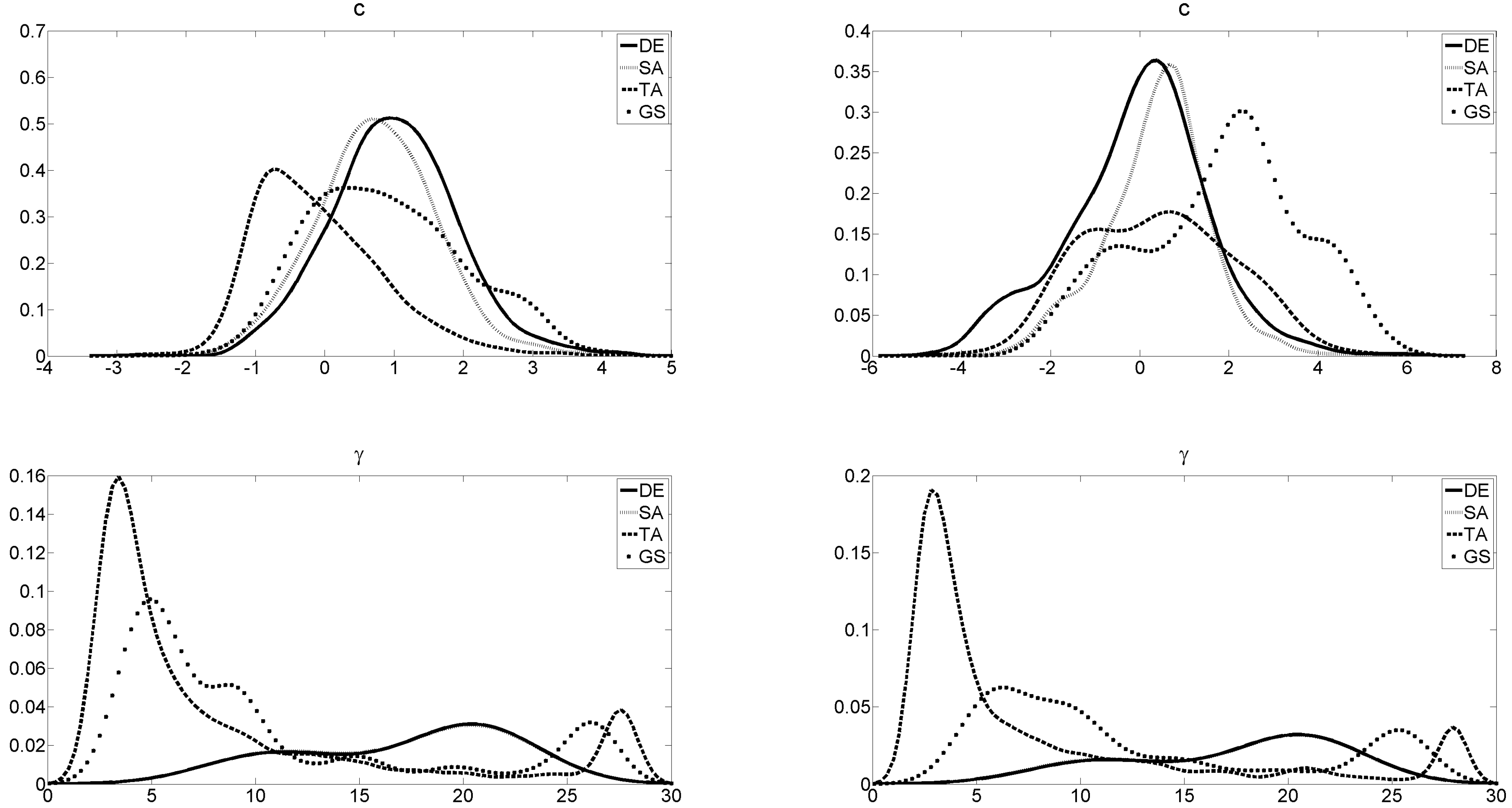
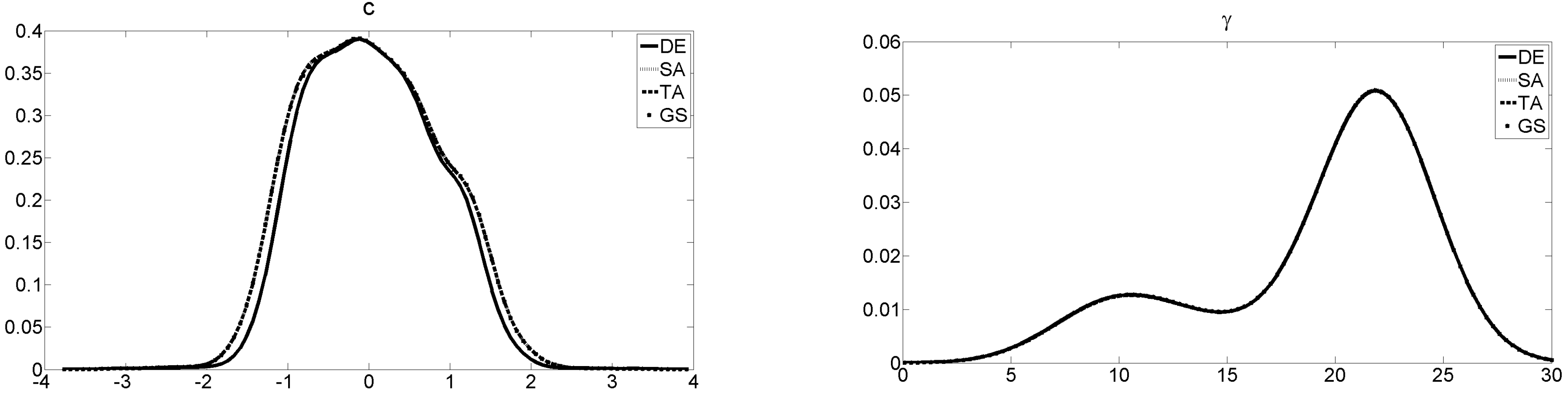
To sum up, all starting-value search procedures work equally well in the equation-by-equation approach. The heuristics, DE somewhat more pronounced than the others, are already quite successful in the starting-value search. As can be seen from Figure 1, the parameter estimates for Γ and C confirm these outcomes as the curves are practically identical.16 The figure refers to the first equation for VSTAR1-1 but the outcomes for the other equation as well as VSTAR1-2 are similar.17 In more than 95% of the simulated cases, the parameter estimates do not differ by more than 0.01 across all procedures in the simulation runs. This is true for the starting-value search as well as for the optimization.

5.2. Multivariate Starting-Value Search

When an equation-by-equation approach is inefficient or not possible at all due to a single transition function governing all equations, a system-wide estimation is appropriate. There are three types of Vector STAR models which theoretically require a multivariate search and estimation procedure: (i) VSTAR2 and VSTAR3 with zero restrictions in the lag structure; (ii) VSTAR1-3 and VSTAR2-3 with cross-correlated error terms; and (iii) VSTAR3-2 which has a single transition function governing the whole model. In the following, I assess the outcomes of different algorithm for finding starting-values in a multivariate setting. Besides that, I evaluate whether the multivariate search and estimation procedure indeed outperforms the equation-by-equation approach. This might not necessarily be the case in applications with short or moderately long time series. It becomes, however, already infeasible to estimate a four dimensional grid in a reasonable computing time. Therefore, I rely on the grid with a zoom advocated by Yang [20] as a benchmark for the heuristic algorithms to derive starting-values for a multivariate search and estimation strategy in the following.

The results for VSTAR2-1 and VSTAR2-2 will be discussed in SubSection 5.2.1 and for the trivariate VSTAR3-1 process in SubSection 5.2.2. SubSection 5.2.3 presents the outcomes for VSTAR models with cross-correlated errors (VSTAR1-3 and VSTAR2-3), and SubSection 5.2.4 those for VSTAR3-2 with a single transition function.

5.2.1. Bivariate Vector STAR Model with Zero Restrictions

I begin by discussing the outcomes of the algorithms applied to VSTAR2 model with zero restrictions, but uncorrelated errors. I employ both a multivariate and an equation-by-equation approach for the starting-value search.

The results in

Table 4. VSTAR2-1 and -2, equation-by-equation vs. multivariate approach.

	VSTAR2-1				VSTAR2-2
	DE	SA	TA	GS	DE	SA	TA	GS
	Starting-Value Search
Eq.≻Mult.	15.8%	23.5%	99.1%	89.5%	18.1%	25.1%	99.7%	88.5%
Mult.≻Eq.	12.5%	10.6%	0.0%	1.2%	11.0%	9.4%	0.0%	1.9%
	Estimation
Eq.≻Mult.	33.3%	39.7%	57.2%	59.4%	21.2%	29.3%	54.4%	55.1%
Mult.≻Eq.	10.8%	9.6%	14.3%	13.0%	5.1%	4.2%	18.6%	16.6%

Better (≻) means at least 0.05 percent higher loglikelihood.

show that although the multivariate search approach would be efficient, it does not yield clearly better outcomes on average than the equation-by-equation search. This is particularly true for TA and GS, whereas the superiority is less pronounced for SA and DE. Thus, there is already a tendency for the equation-by-equation starting-value approach to perform better than the system-wide search. This result holds and becomes even more obvious for DE and SA after estimating the Vector STAR model. The equation-by-equation approach generates a higher frequency of superior results than the multivariate search.

Thus, the gain of estimating Vector STAR models with zero restrictions system-wide is not pronounced in this application. Even if the results were completely identical, the equation-by-equation approach would be preferable due to a shorter execution time.18 Eventually, one could force the multivariate approach to generate better results if one increased the number of likelihood evaluations. This, however, is not in line with the aim of the study which intends to provide an easily applicable modeling strategy. The equation-by-equation methods seem to search more effectively through the parameter space than their system-wide counterparts. The error of not taking the covariance matrix into account in the search procedure is negligible. From the applied point of view, this is a useful result.

Next, I assess the different equation-by-equation starting-value search methods by pairwise comparisons. To begin with, the results support those shown in SubSection 5.1 for the equation-by-equation procedure applied to VSTAR1. The algorithms for finding starting-values do not yield remarkable differences, where SA, TA and DE slightly outperform GS in the starting-value search (see

Table B1. VSTAR2-1 and -2, equation-by-equation search—frequency of superior results.

	VSTAR2-1				VSTAR2-2
	DE	SA	TA	GS	DE	SA	TA	GS
	Starting-Value Search
DE	-	0.12%	0.12%	2.64%	-	0.12%	0.12%	3.48%
SA	0.30%	-	0.00%	2.68%	0.34%	-	0.02%	3.36%
TA	0.30%	0.00%	-	2.68%	0.36%	0.02%	-	3.42%
GS	0.38%	0.22%	0.22%	-	0.42%	0.12%	0.14%	-
	NLS Estimation
DE	-	0.20%	0.46%	0.20%	-	0.20%	0.36%	0.36%
SA	0.28%	-	0.26%	0.16%	0.20%	-	0.20%	0.26%
TA	0.28%	0.00%	-	0.16%	0.18%	0.02%	-	0.24%
GS	0.40%	0.34%	0.58%	-	0.40%	0.32%	0.44%	-

Row better than column. Better means at least 0.05 percent higher loglikelihood.

in Appendix B). After the optimization, the outcomes also show the same pattern as in the previous section. In principle, all methods could be used to find good initial values for bivariate Vector STAR models that contain zero restrictions but uncorrelated error terms.19

To sum up, the gain—in terms of loglikelihood improvement—of the derivative-based algorithm is larger for the grid search than for the heuristics. The heuristics are more successful and slightly superior in the starting-value search. After the derivative-based optimization algorithm is carried out, however, the differences are reduced, implying that GS is able to obtain the same optimum as the heuristics.

5.2.2. Trivariate VSTAR Model with Zero Restrictions

In the following, I consider a higher-dimensional (trivariate) Vector STAR model with zero restrictions and equation-specific transition functions (VSTAR3-1). The results for VSTAR3-1 differ to some extent from the ones shown before.

From

Table 5. VSTAR3-1, equation-by-equation vs. multivariate approach.

	Starting-Value Search				ML Estimation
	DE	SA	TA	GS	DE	SA	TA	GS
Eq.≻Mult.	74.9%	87.9%	100.0%	89.3%	42.4%	48.7%	37.4%	32.7%
Mult.≻Eq.	11.6%	6.8%	0.0%	7.0%	37.6%	31.2%	21.6%	26.9%

Better (≻) means at least 0.05 percent higher loglikelihood.

can be observed that regarding the starting-value search, the equation-by-equation approach is on average preferable for all algorithms. The advantage becomes smaller after the ML estimation, but still for TA and SA a clear superiority of the equation-by-equation approach is maintained. For DE and GS the multivariate search is only slightly inferior on average. The distinction is comparatively small which might not be seen as a clear indication for the equation-by-equation search. Yet, having in mind that the multivariate procedure is associated with a higher computational load, equation-by-equation search appears preferable.

This is again a useful result from an applied perspective: even a more complex model does not necessarily require a multivariate, time-consuming search procedure. Equation-by-equation starting-value search obtains better or sufficiently good starting-values.

Table 6. VSTAR3-1, equation-by-equation search—frequency of superior results.

	Starting-Value Search				ML Estimation
	DE	SA	TA	GS	DE	SA	TA	GS
DE	-	0.14%	0.14%	5.74%	-	0.30%	0.30%	4.14%
SA	0.50%	-	0.00%	5.72%	1.12%	-	0.40%	4.62%
TA	0.50%	0.00%	-	5.72%	1.94%	1.20%	-	5.38%
GS	0.72%	0.30%	0.30%	-	1.72%	1.40%	1.32%	-

Row better than column. Better means at least 0.05 percent higher loglikelihood.

contains results for the individual algorithms. They indicate that the heuristics perform slightly better in the starting-value search than the grid search. However—in contrast to the results derived in the previous subsections—this advantage does not become negligible after ML estimation. The grid search does not always find the best optimum. In 4%–5% GS yields inferior results. Obviously, the inflexibility of the grid in contrast to the heuristic search space is not compensated by an optimization algorithm in a more complex, trivariate process.

To sum up, when the dimension of the model is increased from two to three, the GS performs slightly worse than the heuristics. There is, however, no clear winner of the starting-value search procedure across heuristics. The results differ from the previous ones in SubSection 5.2.1 in one main respect: GS yields slightly worse results also for the final estimates. Although the search problem becomes more complex, an equation-by-equation search equipped with a derivative-based algorithm can handle this optimization problem sufficiently well.

Moreover, a derivative-based algorithm is clearly necessary to improve the loglikelihood derived by the starting-value search which can be seen from

Table 7. VSTAR3-1, comparison of starting-value search and estimation.

	(i)	(ii)
DE	72.94%	0.00%
SA	73.02%	0.02%
TA	73.02%	0.00%
GS	73.42%	0.02%

(i) Estimated loglikelihood at least 0.01 percent better than starting-value search; (ii) Identical results of estimation and starting-value search (up to the fourth decimal).

. In around 73% of the simulation runs the estimated value is better than the loglikelihood value obtained by the starting-value search. This is independent from the procedure used and contrast to the previous results.

5.2.3. Bivariate Vector STAR Model with Cross-Correlated Errors

The second type of Vector STAR models which theoretically require a multivariate search and estimation procedure are those with cross-correlated error terms (VSTAR1-3 and VSTAR2-3). As can be seen directly from

Table 8. VSTAR1-3 and 2-3, equation-by-equation vs. multivariate approach.

	VSTAR1-3				VSTAR2-3
	DE	SA	TA	GS	DE	SA	TA	GS
	Starting-Value Search
Eq.≻Mult.	0.0%	0.0%	1.0%	0.5%	0.0%	0.0%	3.5%	0.0%
Mult.≻Eq.	100.0%	100.0%	99.0%	99.5%	100.0%	100.0%	96.5%	100.0%
	ML Estimation
Eq.≻Mult.	1.6%	2.6%	12.6%	11.0%	0.8%	2.0%	11.5%	3.7%
Mult.≻Eq.	95.2%	94.2%	82.3%	84.5%	94.0%	92.8%	81.4%	89.5%

Better (≻) means at least 0.05 percent higher loglikelihood.

, the equation-by-equation search procedure is not superior anymore in this setting. This is in contrast to the processes that only contain zero restrictions. The system approach outperforms the equation-by-equation search in almost every simulation run. Consequently, for a Vector STAR model with cross-correlated errors the effectiveness of a method that does not take into account the covariance-matrix in the starting-value search is clearly reduced. After the ML estimation, the superiority of the system-wide search is still significantly evident, although the magnitude decreases slightly.

When it comes to the performance of the algorithms, the multivariate starting-value search yields distinct results than the equation-by-equation approach across procedures. This is obvious from Figure 2 by considering the parameter estimates (γ and c) showing diverging results between the search procedures. The estimates vary from one algorithm to the next with the exception of SA and DE.20 The latter procedures yield quite similar parameter estimates, specifically for γ. This is in contrast to the results from the previous section where besides the loglikelihood values also the final parameter estimates coincide.

Table 9. VSTAR1-3 and 2-3, multivariate search—frequency of superior results.

	VSTAR1-3				VSTAR2-3
	DE	SA	TA	GS	DE	SA	TA	GS
	Starting-Value Search
DE	-	29.30%	99.90%	89.90%	-	49.00%	100.00%	78.40%
SA	9.00%	-	99.90%	88.90%	4.90%	-	100.00%	72.90%
TA	0.00%	0.00%	-	17.00%	0.00%	0.00%	-	3.10%
GS	2.00%	3.10%	81.60%	-	5.80%	15.50%	96.70%	-
	ML Estimation
DE	-	25.90%	53.20%	49.90%	-	33.00%	42.70%	35.50%
SA	10.10%	-	51.80%	48.80%	8.50%	-	41.10%	32.80%
TA	18.90%	23.00%	-	25.40%	17.60%	25.20%	-	16.60%
GS	19.30%	22.90%	31.10%	-	17.90%	27.30%	28.30%	-

Row better than column. Better means at least 0.05 percent higher loglikelihood.

reports values of the measure of superiority. They suggest that TA is inferior to the other algorithms. In almost all simulation runs it generates lower loglikelihood values than the other algorithms. Although the grid with a zoom does not yield very convincing results either, it still beats TA in 80%–95%. However, the grid with a zoom is also clearly outperformed by DE and SA in 70%–90% of the simulations runs. DE in particular seems to be very successful. It can be regarded as the best starting-value search procedure assessing solely the loglikelihood values of the starting-value search procedures.

The latter result still holds after the optimization which is the meaningful statistic. Yet, the clarity of the results somewhat decreases. TA remains the most unfavorable starting-value search procedure and does not converge to a good optimum. The search procedure does not seem to be very effective which may be due to an inefficient acceptance criterion. This could stem from a threshold sequence which may not allow for large impairments. Hence, the final outcome could be then a local optimum. DE and SA still perform better than GS grid with a zoom in around 32%–50% of the simulation runs, whereas GS features a clearly lower frequency of superior results w.r.t. SA and DE (only 17%–27%).

A conclusion from this is that the grid search with zoom has a tendency to find an inferior local optimum, which does not help the optimization algorithm to converge to global or at least to a superior local optimum. This argument receives support from the results in

Table 10. VSTAR1-3 and 2-3, comparison of starting-value search and estimation.

	(i)		(ii)
	VSTAR1-3	VSTAR2-3	VSTAR1-3	VSTAR2-3
DE	17.80%	29.70%	80.70%	68.10%
SA	20.40%	34.40%	78.90%	64.90%
TA	79.60%	88.00%	20.40%	12.00%
GS	66.60%	67.30%	30.20%	26.20%

(i) Estimated loglikelihood at least 0.01 percent better than starting-value search; (ii) Identical results of estimation and starting-value search (up to the fourth decimal).

. Although the optimized loglikelihood is in more than 66% at least 0.01 percent better than the starting-value search, the final outcomes are still clearly inferior than those of DE and SA. Hence, the derivative-based algorithm does not help the GS either in obtaining better results. Zooming-in by means of a grid search may rather find a local than a global optimum.

Overall, SA and DE yield the best outcomes for final estimates with a slight edge for DE. From

Table 11. VSTAR1-3 and 2-3, multivariate search—best procedure.

	(a)		(b)
	VSTAR1-3	VSTAR2-3	VSTAR1-3	VSTAR2-3
DE	1290	1112	12.6%	11.1%
SA	1107	824	4.3%	3.4%
TA	673	594	6.9%	4.7%
GS	733	735	6.3%	4.4%

(a) Total number of superior outcomes (better than at least one); (b) Frequency of superior outcomes across all procedures (better than all).

it is seen that DE obtains the highest amount of superior outcomes both overall and across all procedures. DE—belonging to the class of population based methods—updates the whole set of potential solution simultaneously and by that seems to be more successful than the other algorithms.

The results are reinforced by evaluating the magnitude of inferiority. Thereby, I assess by how much an algorithm is inferior if it already obtains a lower loglikelihood value than another algorithm. On average TA and GS with a zoom yield a clearly lower likelihood than SA and DE, if they are already worse than SA and DE (See

Table B2. VSTAR1-3 and 2-3, multivariate search—magnitude of inferiority.

	VSTAR1-3				VSTAR2-3
	DE	SA	TA	GS	DE	SA	TA	GS
	Mean of Worse Results
DE	-	−0.128	−0.448	−0.455	-	−0.122	−0.347	−0.292
SA	−0.168	-	−0.439	−0.451	−0.175	-	−0.351	−0.303
TA	−1.825	−1.843	-	−2.098	−2.347	−2.385	-	−3.010
GS	−1.487	−1.486	−1.656	-	−0.937	−0.955	−1.148	-
	1% Percentile of Worse Results
DE	-	−0.885	−3.786	−3.585	-	−0.634	−3.346	−2.868
SA	−1.155	-	−3.548	−3.242	−0.773	-	−2.742	−2.303
TA	−6.859	−6.871	-	−7.849	−13.017	−13.335	-	−15.353
GS	−8.253	−8.237	−9.750	-	−6.178	−6.959	−9.411	-

Row is at least 0.05 percent worse than column. Mean and 1% percentile of (pairwise) differences of the loglikelihood values if an algorithm yields already a 0.05 lower loglikelihood than another one.

in Appendix B). Hence, GS and TA miss the optimum found by DE and SA by much more than the other way round. The magnitude of inferiority indicates once more that SA and DE are preferable.

5.2.4. Trivariate VSTAR Model with Single Transition Function

Finally, I describe the results of the VSTAR3-2 which is a trivariate Vector STAR model with zero restrictions and one transition function governing the whole system. This makes a multivariate search procedure inevitable. Because only two parameters have to be optimized, I reduce the number of likelihood evaluations and use a normal (equation-by-equation) grid search implementation. The iterations of the heuristics are also decreased to the equation-by-equation set-up and their parameters are adjusted accordingly. Due to the single transition function, a FGLS estimation instead of OLS is applied in the starting-value search for all algorithms. When it comes to estimation, ML instead of NLS has to be used for the latter reason as well.

As can be seen from

Table 12. VSTAR3-2, multivariate search—frequency of superior results.

	Starting-Value Search				ML Estimation
	DE	SA	TA	GS	DE	SA	TA	GS
DE	-	0.00%	52.10%	1.70%	-	0.00%	12.80%	1.70%
SA	0.00%	-	51.80%	1.60%	0.00%	-	12.80%	1.60%
TA	0.00%	0.00%	-	0.30%	0.00%	0.00%	-	1.10%
GS	0.00%	0.00%	51.20%	-	0.00%	0.00%	12.40%	-

Row better than column. Better means at least 0.05 percent higher loglikelihood.

, SA and DE are particulary successful. GS also yields convincing results but is slightly worse than DE and SA, whereas TA clearly ends up in the worst outcomes. In more than 50% the initial values obtained are inferior than those of the other algorithms. This frequency is reduced after ML estimation, but still holds of considerable magnitude. Hence, GS, SA and DE seem to perform best with a slight edge for DE and SA.

In summary, DE and SA are the preferable starting-value search methods for a higher-dimensional Vector STAR process with one transition function requiring a multivariate search.

6. Conclusion

The estimation outcome of Vector STAR models crucially relies on good starting-values. Initializing a derivative-based algorithm with starting-values close to the global optimum or at least close to a useful local optimum helps the algorithm to cover the remaining distance to the nearest optimum. Based on a comprehensive Monte Carlo simulation exercise, I compare different procedures, namely grid search (GS), simulated annealing (SA), differential evolution (DE), and threshold accepting (TA), for finding starting-values in Vector STAR models. The results are as follows.

For bivariate Vector STAR models that do not exhibit cross-correlation across error terms—no matter whether the process contains zero restrictions—equation-by-equation starting-value search is preferable. In this approach, differences across procedures are negligible. In the case of heuristics (DE, SA, and TA), the starting-value search is only slightly improved by the derivative-based algorithm, indicating that they are already quite successful in finding starting-values. GS benefits more from a derivative-based optimization procedure.

The optimization in a higher-dimensional Vector STAR model can still be handled sufficiently well by an equation-by-equation search approach followed by a derivative-based algorithm. Differences to the bivariate model are that (i) the derivative-based algorithm clearly improves the outcome obtained by the starting-value search of all procedures; and (ii) the heuristic methods obtain slightly better results than the grid search. This may stem from the more flexible search space of heuristics.

In case of a higher-dimensional Vector STAR model which is governed by one transition function, TA yields clearly the most unfavourable outcomes. SA and DE slightly improve parameter estimation compared to GS.

If the error terms are cross-correlated, a multivariate starting-value search procedure is preferable. TA and the GS with a zoom do not yield convincing results compared to SA and DE. The latter two seem to be the best starting-value search methods for those Vector STAR models for which a multivariate procedure is superior with a slight edge for DE. The GS with a zoom and TA show a tendency to find inferior optima rather than a global or at least superior local optimum.

The following procedure could be adopted for an empirical application. If the Vector STAR model has a single transition function, SA and DE are preferable. However, if the transition function is equation-specific, one should initially check whether the errors of the Vector STAR model are cross-correlated. This could be done statistically as well as by assessing whether correlation across equations are economically reasonable. If they are not correlated, all methods achieve equally well results unless the model has more than two dimensions. Then, one should rather apply a heuristic method than the grid search. In an empirical application of a multivariate Vector STAR model with cross-correlated errors, one should use DE or SA for finding starting-values to reach a good optimum.