A GMM-Based Test for Normal Disturbances of the Heckman Sample Selection Model

Abstract

The Heckman sample selection model relies on the assumption of normal and homoskedastic disturbances. However, before considering more general, alternative semiparametric models that do not need the normality assumption, it seems useful to test this assumption. Following Meijer and Wansbeek (2007), the present contribution derives a GMM-based pseudo-score LM test on whether the third and fourth moments of the disturbances of the outcome equation of the Heckman model conform to those implied by the truncated normal distribution. The test is easy to calculate and in Monte Carlo simulations it shows good performance for sample sizes of 1000 or larger.

1. Introduction

The assumption of bivariate normal and homoskedastic disturbances is a prerequisite for the consistency of the maximum likelihood estimator of the Heckman sample selection model. Moreover, some studies focus on the prediction of counterfactuals based on the Heckman sample selection model taking into account both changes in participation and outcome, which is often only feasible under the assumption of bivariate normality.1 Lastly, under the assumption of bivariate normality one can the estimate the Heckman sample selection model by maximum likelihood methods that are less sensitive to weak exclusion restrictions.

Before employing alternative semiparametric estimators that do not need the normality assumption (see e.g., Newey, 2009 [3]), it seems useful to test the underlying normality assumption of sample selection models. So far, the literature offers several approaches to test this hypothesis.2 Bera et. al., (1984) [6] develop an LM test for normality of the disturbances in the general Pearson framework, which implies testing the moments up to order four. Lee (1984) [7] proposes Lagrangian multiplier tests within the bivariate Edgeworth series of distributions. Van der Klaauw and Koning (1993) [8] derive LR tests in a similar setting, while Montes-Rojas (2011) [9] proposes LM and $C\left(\alpha \right)$ tests that are likewise based on bivariate Edgeworth series expansions, but robust to local misspecification in nuisance distributional parameters. In general, these approaches tend to lead to complicated test statistics that are sometimes difficult to implement in standard econometric software. More importantly, some of these tests for bivariate normality seem to exhibit unsatisfactory performance in Monte Carlo simulations and are rejected too often in small to medium samples sizes, especially if the parameter of the Mills’ ratio is high in absolute value (see e.g., Montes-Rojas, 2011 [9], Table 1). This motivates Montes-Rojas (2011) [9] to focus on the assumptions of the two-step estimator that requires less restrictive assumptions, namely a normal marginal distribution of the disturbances of the selection equation and a linear conditional expectation of the disturbances of the outcome equation. He proposes to test for marginal normality and linearity of the conditional expectation of outcome model separately and shows that the corresponding locally size-robust test statistics based on the two-step estimator perform well in terms size and power .

In a possibly neglected, but very valuable paper, Meijer and Wansbeek (2007) [10] embed the two-step estimator of the Heckman sample selection model in a GMM-framework. In addition, they argue that within this framework it is easily possible to add moment conditions for designing Wald tests in order to check the assumption of bivariate normality and homoskedasticity of the disturbances. Their approach does not attempt to develop a most powerful test, rather they intended to design a relatively simple test for normality that can be used as an alternative to the existing tests. The test can be interpreted as a conditional moment test and checks whether the third and fourth moments of the disturbances of the outcome equation of the Heckman model conform to those implied by the truncated normal distribution. For $H_0$ to hold, the test in addition requires normally distributed disturbances of the selection equation and the absence of heteroskedasticity in both the outcome and the selection equation.

Meijer and Wansbeek (2007) [10] do not explicitly derive the corresponding test statistic nor do they provide Monte Carlo simulations on its performances in finite samples. The present contribution takes up their approach arguing that a GMM based pseudo-score LM test is well suited to test the hypothesis of bivariate normality and is easy to calculate. The derived LM test is similar to the widely used Jarque and Bera LM test (1980) [11], and in the absence of sample selection reverts to their LM test statistic. Monte Carlo simulations show good performance of the proposed test for samples of sizes of 1000 or larger, especially if a powerful exclusion restriction is available.

2. The GMM Based Pseudo-Score LM Test for Normality

In a cross-section of n units the Heckman (1979) [12] sample selection model is given as

$$\begin{array}{ccc}\hfill y_{1i}^{*}& =& z_i^{\prime }\gamma +u_{1i}\hfill \\ \hfill y_{2i}^{*}& =& x_i^{\prime }\beta +u_{2i}\hfill \\ \hfill d_i& =& \left\{\begin{array}{cc}1& \text{if}{y}_{1i}^{*}>0\\ 0& \text{otherwise}\end{array}\right.\hfill \\ \hfill y_{2i}& =& \left\{\begin{array}{cc}{y}_{2i}^{*}\hfill & \text{if}{d}_i=1\\ \text{unobserved}\hfill & \text{if}{d}_i=0\end{array}\right.\hfill \end{array}$$

where $y_{1i}^{*}$ and $y_{2i}^{*}$ denote latent random variables. The outcome variable, $y_{2i}^{*},$ is observed if the latent variable $y_{1i}^{*}>0$ or, equivalently, if $d_i=1$. $z_i$ is a $k_1\times 1$ vector containing the exogenous variables of the selection equation and $x_i$ is the $k_2\times 1$ vector of the exogenous variables of the outcome equation. $z_i$ may include the variables in $x_i,$ but also additional ones so that an exclusion restriction holds. γ and β denote the corresponding parameter vectors. Under $H_0$ the disturbances are assumed to be distributed as bivariate normal, i.e.,

$$\left(\left[\begin{array}{c}{u}_{1i}\\ u_{2i}\end{array}\right]|x_i,z_i\right)\sim N\left(\left[\begin{array}{c}0\\ 0\end{array}\right],\left[\begin{array}{cc}1& \tau \\ \tau & {\sigma }^2\end{array}\right]\right)$$

It is easy to show that under these assumptions

$$\begin{array}{ccc}\hfill p_i& \equiv & E\left[d_i\right]=\Phi \left(z_i^{\prime }\gamma \right)\hfill \\ \hfill {\lambda }_i& \equiv & E\left[u_{1i}\right|u_{1i}\ge -z_i^{\prime }\gamma ]=\frac{\varphi (-z_i^{\prime }\gamma )}{1-\Phi (-z_i^{\prime }\gamma )}=\frac{\varphi \left(z_i^{\prime }\gamma \right)}{\Phi \left(z_i^{\prime }\gamma \right)}\hfill \end{array}$$

where ${\lambda }_i$ denotes the inverse Mills’ ratio. Under the normal assumption one can specify $u_{2i}=\tau u_{1i}+{\epsilon }_i$ so that ${\epsilon }_i\sim iid N(0,{\sigma }^2-{\tau }^2)$. ${\epsilon }_i$ is independent of $u_{1i}$ as $E\left[{\epsilon }_i{u}_{1i}\right]=E\left[\left(u_{2i}-\tau u_{1i}\right)u_{1i}\right]=\tau -\tau =0$. Since $E\left[u_{1i}\right|d_i=1]={\lambda }_i$, it holds that $E[\tau (u_{1i}-{\lambda }_i)+{\epsilon }_i|d_i=1]=0$. Therefore, the two-step Heckman sample selection model includes the estimated inverse Mills’ ratio in the outcome equation as an additional regressor. For the observed outcome at $d_i=1$ the model can be written as

$$\begin{array}{ccc}\hfill y_{2i}^{*}& =& x_i^{\prime }\beta +\tau {\lambda }_i+\tau \left(u_{1i}-{\lambda }_i\right)+{\epsilon }_i\hfill \\ & \equiv & w_i^{\prime }\alpha +\tau v_i+{\epsilon }_i\hfill \end{array}$$

(1)

where $v_i=u_{1i}-{\lambda }_i$ and $E\left[y_{2i}^{*}\right|d_i=1]=x_i^{\prime }\beta +\tau {\lambda }_i.$

Meijer and Wansbeek (2007) [10] embed the two-step Heckman sample selection estimator in a GMM framework and demonstrate that the estimation can be based on

$$\begin{array}{ccc}\hfill h_{1,1i(k_1\times 1)}\left({\theta }_1\right)& \equiv & \frac{(d_i-p_i){\varphi }_i}{p_i(1-p_i)}{z}_i\hfill \\ \hfill h_{1,2i(k_2\times 1)}\left({\theta }_1\right)& \equiv & d_i{w}_i(y_i-w_i^{\prime }\alpha )=d_i{w}_i(\tau v_i+{\epsilon }_i)\hfill \\ \hfill h_{1,3i(1\times 1)}\left({\theta }_1\right)& \equiv & d_i\left[{(y_i-w_i^{\prime }\alpha )}^2-{\phi }_{2,i}\right]=d_i\left[{({\epsilon }_i+\tau v_i)}^2-{\phi }_{2,i}\right]\hfill \end{array}$$

where ${\theta }_1={({\gamma }^{\prime },{\beta }^{\prime },\tau ,\sigma )}^{\prime }$ and ${\phi }_{k,i}=E\left[{\left(\tau v_i+{\epsilon }_i\right)}^k|d_i=1\right],k=2,3,4.$ Note, there are as many parameters as moment conditions and the model is just-identified.

The first set of moment equations is based on ${\overline{h}}_{1,1}\left({\theta }_1\right)=\frac{1}{n}{\sum }_{i=1}^n{h}_{1,1i}\left({\theta }_1\right)$ and refers to the score of the Probit model. Since these moment conditions do not include the parameters entering $h_{1,2i}$ and $h_{1,3i}$ (i.e., ${\beta }^{\prime },\tau ,\sigma$) and are exactly identified, estimation can proceed in steps: In the first step, one can solve $\frac{1}{n}{\sum }_{i=1}^n{h}_{1,1i}\left(\widehat{\gamma }\right)=0$ and in the second step one solves the sample moment condition ${\overline{h}}_{1,2}\left({\theta }_1\right)=\frac{1}{n}{\sum }_{i=1}^n\left[h_{1,2i}({\widehat{\gamma }}^{\prime },{\widehat{\beta }}^{\prime },\widehat{\tau })\right]=0$ using the estimated $\widehat{\gamma }$ derived in the first stage. This leads to the two-step Heckman estimator, which first estimates a Probit model, inserts the estimated Mills’ ratio ${\widehat{\lambda }}_i$ as additional regressor in the outcome equation and applies OLS. Lastly, from ${\overline{h}}_{1,3}\left({\theta }_1\right)=\frac{1}{n}\sum h_{1,3i}({\widehat{\gamma }}^{\prime },{\widehat{\beta }}^{\prime },\widehat{\tau },\widehat{\sigma })=0$ one can obtain an estimator of ${\sigma }^2.$

As Meijer and Wansbeek (2007) [10] remark, a rough and simple test for normality can be based on two additional moment conditions that allow comparing the third and fourth moments of the estimated residuals of the outcome equation, $y_i-w_i^{\prime }\widehat{\alpha }$, with their theoretical counterparts based on the truncated normal distribution. These moment conditions use

$$\begin{array}{ccc}\hfill h_{2,1i(1\times 1)}({\theta }_1,{\theta }_2)& \equiv & d_i\left[{(y_i-w_i^{\prime }\alpha )}^3-{\phi }_{3,i}-\xi \right]=d_i\left[{(\tau v_i+{\epsilon }_i)}^3-{\phi }_{3,i}-\xi \right]\hfill \\ \hfill h_{2,2i(1\times 1)}({\theta }_1,{\theta }_2)& \equiv & d_i\left[{(y_i-w_i^{\prime }\alpha )}^4-{\phi }_{4,i}-\kappa \right]=d_i\left[{(\tau v_i+{\epsilon }_i)}^4-{\phi }_{4,i}-\kappa \right]\hfill \end{array}$$

Thereby, ${\theta }_2=(\xi ,\kappa )$ denotes additional parameters that are zero under normality. More importantly, under $H_0$ the expectations ${\phi }_{k,i}$ can be derived recursively from the moments of the truncated normal distribution as shown in the Appendix (see alsoMeijer and Wansbeek, 2007, pp. 45–46) [10]. In general, these moments depend on the parameters ${\theta }_1$ and, especially, on the inverse Mills’ ratio ${\lambda }_i$ and the parameter τ.

To detect violations of the normality assumption, one can test $H_0:\xi =0$ and $\kappa =0$ vs. $H_0:\xi \ne 0$ and/or $\kappa \ne 0.$ Although this hypothesis checks the third and fourth moments of the disturbances of the two-step outcome Equation (1), it can only be true if ${\phi }_{3,i}$ and ${\phi }_{4,i}$ are the correct expected values. Therefore, the test additionally requires the moment conditions $E\left[h_{1,1i}\right]=0$ and $E[h_{1,2i}=0]$ to hold so that the parameters of both the selection equation and the outcome equation are consistently estimated. The present hypothesis is somewhat more restrictive than that tested, e.g., in Montes-Rojas (2011) [9], who emphasizes that the Heckman two-step estimator is robust to distributional misspecification if (i) the marginal distribution of $u_{1i}$ is normal and (ii) $E\left[u_{2i}\right|u_{1i}]=\tau u_{1i}$, i.e., the conditional expectation is linear.3

In addition, $H_0$ also requires the absence of heteroskedasticity ( see Meijer and Wansbeek, 2007, p. 46 ) [10]. To give an example, assume that $u_{2i}=\tau u_{1i}+{\epsilon }_i$ and $u_{2i}$ are bivariate normal, but the variances of ${\epsilon }_i$ differ across i and are given as ${\sigma }_i^2-{\tau }^2$ (see also the DGP6 in the Monte Carlo set-up below and the excess kurtosis of DGP6 in Table 1 below). Then, it follows that ${\phi }_{k,i}={\sum }_{j=0}^k\left(\genfrac{}{}{0pt}{}{k}{j}\right)E\left[{\epsilon }_i^{k-j}\right]{\tau }^j{\psi }_{j,i},$ where ${\psi }_{k,i}\equiv E[\left(v_i^k\right|d_i=1]={\sum }_{j=0}^k{(-1)}^j\left(\genfrac{}{}{0pt}{}{k}{j}\right){\mu }_{j,i}{\lambda }_i^{k-j}$ and ${\mu }_{j,i}=E\left[u_{1i}^k\right|u_{1i}>-z_i^{\prime }\gamma ]$ (see the Appendix). In this case, we have $E\left[{\epsilon }_i^2\right]={\sigma }_i^2-{\tau }^2$ and $E\left[{\epsilon }_i^4\right]=3{\left({\sigma }_i^2-{\tau }^2\right)}^2$, while the corresponding uneven moments are zero. Hence, under heteroskedasticity ${\phi }_{4,i}$ differs from that obtained under $H_0$ which assumes $E\left[{\epsilon }_i^2\right]={\sigma }^2-{\tau }^2$ and $E\left[{\epsilon }_i^4\right]=3{({\sigma }^2-{\tau }^2)}^2$ and the population moment condition $E\left[h_{2,2i}({\theta }_1,{\theta }_2)\right]=0$ is violated. Hence, a test based on these moments should also be able to detect heteroskedasticity, although not in the most efficient way.

Applying a pseudo-score LM test (Newey and West, 1987 [13]; Hall, 2005 [14]), in this GMM-framework leads to a ${\chi }^2\left(2\right)$-test statistic that can be calculated easily. In order to derive the LM test statistic, define $\overline{h}\left(\theta \right)=\frac{1}{n}{\sum }_{i=1}^n{h}_i\left(\theta \right)$ and $\overline{\Psi }\left(\theta \right)=\frac{1}{n}{\sum }_{i=1}^n{h}_i\left(\theta \right)h_i{\left(\theta \right)}^{\prime }$, where $h_i\left(\theta \right)\equiv {(h_{1,1i}^{\prime },h_{1,2i}^{\prime },h_{1,3i},h_{2,1i},h_{2,2i})}^{\prime }$. It is assumed that ${\Psi }_0$ = $pli{m}_{n\to \infty }\overline{\Psi }\left({\theta }_0\right)$ exists, is positive definite and invertible. Under standard assumptions, it holds that

$$\begin{array}{c}{n}^{1/2}\overline{h}\left({\theta }_0\right)\stackrel{d}{\to }N(0,{\Psi }_0)\hfill \\ n^{1/2}(\widehat{\theta }-{\theta }_0)\stackrel{d}{\to }N(0,A_0)\hfill \end{array}$$

where the subscript 0 indicates that $H_0$ is assumed. Thereby, $A_0=G_0^{-1}{\Psi }_0{\left(G_0^{-1}\right)}^{\prime }$ and $G_0$ is the probability limit of $\overline{G}\left({\theta }_0\right)=\frac{1}{n}{\sum }_{i=1}^n{\left.\frac{\partial h\left(\theta \right)}{\partial \theta }\right|}_{\theta ={\theta }_0}$. Note, $\overline{G}\left({\theta }_0\right)$ is invertible as the model is just-identified.

Under $H_0$ the moment conditions $E[h_{2,i}({\theta }_1,{\theta }_2),\xi ,\kappa ],h_{2,i}({\theta }_1,{\theta }_2)\equiv {(h_{2,1i},h_{2,2i})}^{\prime }$ referring to the third and fourth moments of the outcome equation are zero at $\xi =0$ and $\kappa =0$ and the separability result in Ahn and Schmidt (1995, Section 4) [15] can be applied. Denoting the restricted estimates under $H_0$ by a tilde, using the invertibility of $\overline{G}\left(\tilde{\theta }\right)$ and the partitioned inverse of ${\Psi }_n\left(\tilde{\theta }\right)=E\left[\overline{\Psi }\left(\tilde{\theta }\right)\right]$, the pseudo-score LM test statistic can be derived as (see the Appendix for details):

$$LM\left(\tilde{\theta }\right)=n{\overline{h}}_2^{\prime }\left(\tilde{\theta }\right){\left({\Psi }_{n,22}\left(\tilde{\theta }\right)-{\Psi }_{n,21}\left(\tilde{\theta }\right){\Psi }_{n,11}{\left(\tilde{\theta }\right)}^{-1}{\Psi }_{n,12}\left(\tilde{\theta }\right)\right)}^{-1}{\overline{h}}_2\left(\tilde{\theta }\right)$$

Thereby, ${\overline{h}}_2\left(\theta \right)=\frac{1}{n}{\sum }_{i=1}^n{h}_{2,i}\left(\theta \right)$ and we use ${\overline{h}}_1^{\prime }\left(\tilde{\theta }\right)=\frac{1}{n}{\sum }_{i=1}^n{h}_{1,i}\left(\tilde{\theta }\right)=0,$ where $h_{1,i}\left(\theta \right)={(h_{1,1i}^{\prime },h_{1,2i}^{\prime },h_{1,3i})}^{\prime }$, as well as the partitioned inverse (see the Appendix)

$$\begin{array}{ccc}\hfill {\Psi }_{n,11}\left(\theta \right)& =& \frac{1}{n}\left[\begin{array}{ccc}{Z}^{\prime }VZ& 0& 0\\ *& W_1^{\prime }{\Sigma }_1{W}_1& \sum _{d_i=1}{w}_i{\phi }_{3,i}\\ *& *& \sum _{d_i=1}\left({\phi }_{4,i}-{\phi }_{2,i}^2\right)\end{array}\right]\hfill \\ \hfill {\Psi }_{n,22}\left(\theta \right)& =& \frac{1}{n}\sum _{i=1}\left[\begin{array}{cc}{p}_i\left({\phi }_{6,i}-{\phi }_{3,i}^2\right)& p_i\left({\phi }_{7,i}-{\phi }_{3,i}{\phi }_{4,i}\right)\\ p_i\left({\phi }_{7,i}-{\phi }_{3,i}{\phi }_{4,i}\right)& p_i\left({\phi }_{8,i}-{\phi }_{4,i}^2\right)\end{array}\right]\hfill \\ \hfill {\Psi }_{n,12}\left(\theta \right)& =& \frac{1}{n}\sum _{i=1}^n\left[\begin{array}{cc}0& 0\\ p_i{w}_i{\phi }_{4,i}& p_i{w}_i{\phi }_{5,i}\\ p_i\left({\phi }_{5,i}-{\phi }_{2,i}{\phi }_{3,i}\right)& p_i\left({\phi }_{6,i}-{\phi }_{4,i}{\phi }_{2,i}\right)\end{array}\right]\hfill \end{array}$$

where $V=diag\left(\frac{{\varphi }_1^2}{p_1(1-p_1)},..,\frac{{\varphi }_n^2}{p_n(1-p_n)}\right), p_i=P(d_i=1), Z_{n\times k_1}={(z_1,...,z_n)}^{\prime }, W_{n\times k_2}={(w_1,...,w_n)}^{\prime },$ and $\Sigma =diag({\phi }_{2,1},...,{\phi }_{2,n})$. ${\Sigma }_1$ is obtained from Σ by deleting all rows and columns referring to $d_i=0$, and similarly $W_1.$ ${\Psi }_n\left(\theta \right)$ can be consistently estimated by plugging in $\tilde{\theta }$. In addition, Meijer and Wansbeek (2007) [10] show that one can substitute $d_i$ for $p_i$ so that only information on the observed units is necessary. Note however, the summation runs over all observations (zero and ones in $d_i$).

Under standard assumptions it follows that under $H_0$ we have $LM\left(\tilde{\theta }\right)\stackrel{d}{\to }{\chi }^2\left(2\right)$ (see Newey and West, 1987, pp. 781–782 [13] and Theorems 5.6 and 5.7 in Hall, 2005 [14]) . In the absence of sample selection ($\tau =0$) it holds that ${\phi }_{3,i}={\phi }_{5,i}=0$, while ${\phi }_{2,i}={\sigma }^2$ and ${\phi }_{4,i}=3{\sigma }^4$ and the LM test statistic reverts to that of Jarque and Bera (1980) [11].

3. Monte Carlo Simulation

Monte Carlo simulations may shed light on the performance of the proposed LM test in finite samples. It is based on a design that has been used previously by van der Klaauw and Koning (1993) [8] and Montes-Rojas (2011) [9], but includes a few modifications. The simulated model is specified as

$$\begin{array}{ccc}\hfill y_{1i}^{*}& =& -1z_{1i}+1x_{2i}-1+u_{1i}\hfill \\ \hfill y_{2i}^{*}& =& 0.5x_{1i}-0.5x_{2i}+1+u_{2i}\hfill \end{array}$$

where for $\rho \in \{-0.8,-0.4,0.4,0.8\}$ and ${\sigma }^2\in \{0.25,1\}.$ The explanatory variables $x_{1i}, x_{2i}$, and $z_{1i}$ are generated as $iid N(0,3),$ $N(0,3)$ and $U(-3,3),$ respectively. With respect to the disturbances, $u_{1i}$, and $u_{2i}$ the following data generating processes are considered. Note DGP1-DGP3 imply $Var\left[u_{1i}\right]=1$ and $Var\left[u_{2i}\right]=0.25.$ In contrast, van der Klaauw and Koning (1993) [8] and Montes-Rojas (2011) [9] consider the case with $Var\left[u_{2i}\right]=5$ and thus receive less precise estimates of the slope parameters of the outcome equation.

• DGP1:
  $(u_{1i},u_{2i})\sim iid N\left(0,\left[\begin{array}{cc}1& 0.5\rho \\ 0.5\rho & 0.25\end{array}\right]\right)$
• DGP2:
  ${\epsilon }_{1i}\sim t\left(10\right), {\epsilon }_{2i}\sim t\left(10\right), {\epsilon }_{1i}$ and ${\epsilon }_{2i}$ being independent.
  $u_{1i}={\epsilon }_{1i}{\left(\frac{10}{8}\right)}^{-1/2}$
  $u_{2i}=\sigma {(1+{\rho }^2)}^{1/2}{\left(\frac{10}{8}\right)}^{-1/2}{\epsilon }_{2i}+\rho \sigma u_{1i}$
  The degrees of freedom are set to 10 to guarantee that the moments up to order 4 exists.
• DGP3:
  ${\epsilon }_{1i}\sim {\chi }^2\left(20\right), {\epsilon }_{2i}\sim {\chi }^2\left(30\right)$
  $u_{1i}=\left({\epsilon }_{1i}-20\right)/\sqrt{40}-20$
  $u_{2i}=\sigma {(1+{\rho }^2)}^{1/2}\left({\epsilon }_{2i}-30\right)/\sqrt{60}+\rho \sigma u_{1i}$
• DGP4:
  ${\epsilon }_{1i}\sim N(0,1), {\epsilon }_{2i}\sim {\chi }^2\left(30\right)$ and are independent.
  $u_{1i}={\epsilon }_{1i}$
  $u_{2i}=\sigma {(1+{\rho }^2)}^{1/2}\left({\epsilon }_{2i}-30\right)/\sqrt{60}+\rho \sigma u_{1i}$
• DGP5:
  ${\epsilon }_{1i}\sim {\chi }^2\left(20\right), {\epsilon }_{3i}\sim N(0,1)$ and are independent.
  $u_{1i}=\left({\epsilon }_{1i}-20\right)/\sqrt{40}-1$
  $u_{2i}=\sigma {(1+{\rho }^2)}^{1/2}{\epsilon }_{2i}+\rho \sigma u_{1i}$
• DGP6:
  ${\epsilon }_{1i}\sim N(0,1), {\epsilon }_{2i}\sim N(0,0.25), {\epsilon }_{1i}$ and ${\epsilon }_{2i}$ being independent.
  $c_i=1+e^{\frac{x_{1i}}{\sqrt{3}}}\left(e^{-\frac{1}{2}}-1\right){\left(e^1-1\right)}^{-\frac{1}{2}}$
  $u_{1i}={\epsilon }_{1i}$
  $u_{2i}=\sigma {(1+{\rho }^2)}^{1/2}\sqrt{c_i}{\epsilon }_{2i}+2\rho u_{1i}$
• DGP7:
  ${\epsilon }_{1i}\sim N(0,1), {\epsilon }_{2i}\sim N(0,1), {\epsilon }_{1i}$ and ${\epsilon }_{2i}$ being independent.
  $c_i=1+e^{\frac{x_{2i}}{\sqrt{3}}}\left(e^{-\frac{1}{2}}-1\right){\left(e^1-1\right)}^{-\frac{1}{2}}$
  $u_{1i}={\epsilon }_{1i}\sqrt{c_i}$
  $u_{2i}=\sigma {(1+{\rho }^2)}^{1/2}{\epsilon }_{2i}+\sigma \rho u_{1i}$

DGP1 serves as a reference to assess the size of the pseudo-score LM test. The second DGP deviates from the bivariate normal in terms of a higher kurtosis, while DGP3 exhibits both higher skewness and kurtosis than the normal. DGP4 allows for deviation from normality in the outcome equation, while keeping the normality assumption in the selection equation. DGP5 reverses this pattern. The disturbances of the outcome equation are normal and those of the selection equation are not. DGP6 and DGP7 introduce heteroskedasticity in either the outcome or the selection equation, respectively. In case of the latter two, the variances of $u_{i1}$ and $u_{i2}$ is normalized to an average of 1 and $0.25$, respectively. Note, the explanatory variables are held fixed in repeated samples.

Overall, for these DGPs four experiments are considered. In the baseline Experiment 1 (first row of the figures of graphs) $37\%$ of the data remain unobserved and in the absence of sample selection the implied $R^2$ amounts to $1-\frac{0.25}{1.75}$ = $0.86$ using $Var\left(u_{2i}\right)=0.25$ and $Var\left(y_{2i}^{*}\right)=1.75$. Experiment 2 (second row of the figures of graphs) analyzed the performance of the Heckman two-step estimator under a weaker exclusion restriction, assuming $z_{1i}\sim iid U(-1,1)$ so that $Var\left(z_{1i}\right)=1/3$: Experiment 3 (third row of the figures of graphs) sets the constant of the outcome equation to zero so that $49\%$ instead of $37\%$ units are unobserved. Lastly, Experiments 4 (fourth row of the figures of graphs) considers a weaker fit in the outcome equation setting $Var\left(u_{2i}\right)=1$ so that in the absence of sample selection we have $R^2=0.43.$

Table 1 summarizes the average variance, skewness and kurtosis of the generated disturbances $u_{1i}$ and $u_{2i}$ under Experiment 1. In DGP2-DGP7, depending on ρ, the average kurtosis of $u_{2i}$ varies between $3.00$ and $5.68$, while the kurtosis of $u_{1i}$ lies between $3.07$ and $3.58$ in DGP5. In the other ones the kurtosis of $u_{1i}$ is held constant taking values $2.99$ (DGPs 1,4 and 6), $3.97$ (DGP2), $3.58$ (DGP3) and $5.71$ (DGP7), respectively. The skewness coefficient of the generated disturbances is zero for all DGPs except for DGP3 with corresponding values of 0.63 ($u_{1i}$) and $-0.21$ to 0.43 ($u_{2i}$) and DGP5 where the skewness of $u_{1i}$ varies between $0.14$ and $0.63$.

Table 1. Variance, Skewness and Kurtosis of the simulated disturbances.

DGP	ρ	$u_1$				$u_2$
		Variance	Skewness	Kurtosis	Variance	Skewness	Kurtosis
1	all	1.00	0.00	2.99	0.25	0.00	2.99
2	−0.8	1.00	0.00	3.97	0.25	0.00	3.52
2	−0.4	1.00	0.00	3.97	0.25	0.00	3.70
2	0.0	1.00	0.00	3.97	0.25	0.00	3.96
2	0.4	1.00	0.00	3.97	0.25	0.00	3.70
2	0.8	1.00	0.00	3.97	0.25	0.00	3.52
3	−0.8	1.00	0.63	3.58	0.25	−0.21	3.29
3	−0.4	1.00	0.63	3.58	0.25	0.35	3.28
3	0.0	1.00	0.63	3.58	0.25	0.51	3.38
3	0.4	1.00	0.63	3.58	0.25	0.43	3.28
3	0.8	1.00	0.63	3.58	0.25	0.43	3.29
4	−0.8	1.00	0.00	2.99	0.25	0.11	3.05
4	−0.4	1.00	0.00	2.99	0.25	0.39	3.27
4	0.0	1.00	0.00	2.99	0.25	0.51	3.38
4	0.4	1.00	0.00	2.99	0.25	0.39	3.27
4	0.8	1.00	0.00	2.99	0.25	0.11	3.04
5	−0.8	1.00	0.63	3.58	0.25	0.00	2.99
5	−0.4	1.00	0.63	3.58	0.25	0.00	2.99
5	0.0	1.00	0.63	3.58	0.25	0.00	2.99
5	0.4	1.00	0.63	3.58	0.25	0.00	2.99
5	0.8	1.00	0.63	3.58	0.25	0.00	2.99
6	−0.8	1.00	0.00	2.99	0.25	0.00	3.34
6	−0.4	1.00	0.00	2.99	0.25	0.00	4.89
6	0.0	1.00	0.00	2.99	0.25	0.00	5.68
6	0.4	1.00	0.00	2.99	0.25	0.00	4.89
6	0.8	1.00	0.00	2.99	0.25	0.00	3.35
7	−0.8	0.99	0.00	5.71	0.25	0.00	4.11
7	−0.4	0.99	0.00	5.71	0.25	0.00	3.06
7	0.0	0.99	0.00	5.71	0.25	0.00	2.99
7	0.4	0.99	0.00	5.71	0.25	0.00	3.06
7	0.8	0.99	0.00	5.71	0.25	0.00	4.11

Table 1. Variance, Skewness and Kurtosis of the simulated disturbances.

DGP	ρ	$u_1$				$u_2$
		Variance	Skewness	Kurtosis	Variance	Skewness	Kurtosis
1	all	1.00	0.00	2.99	0.25	0.00	2.99
2	−0.8	1.00	0.00	3.97	0.25	0.00	3.52
2	−0.4	1.00	0.00	3.97	0.25	0.00	3.70
2	0.0	1.00	0.00	3.97	0.25	0.00	3.96
2	0.4	1.00	0.00	3.97	0.25	0.00	3.70
2	0.8	1.00	0.00	3.97	0.25	0.00	3.52
3	−0.8	1.00	0.63	3.58	0.25	−0.21	3.29
3	−0.4	1.00	0.63	3.58	0.25	0.35	3.28
3	0.0	1.00	0.63	3.58	0.25	0.51	3.38
3	0.4	1.00	0.63	3.58	0.25	0.43	3.28
3	0.8	1.00	0.63	3.58	0.25	0.43	3.29
4	−0.8	1.00	0.00	2.99	0.25	0.11	3.05
4	−0.4	1.00	0.00	2.99	0.25	0.39	3.27
4	0.0	1.00	0.00	2.99	0.25	0.51	3.38
4	0.4	1.00	0.00	2.99	0.25	0.39	3.27
4	0.8	1.00	0.00	2.99	0.25	0.11	3.04
5	−0.8	1.00	0.63	3.58	0.25	0.00	2.99
5	−0.4	1.00	0.63	3.58	0.25	0.00	2.99
5	0.0	1.00	0.63	3.58	0.25	0.00	2.99
5	0.4	1.00	0.63	3.58	0.25	0.00	2.99
5	0.8	1.00	0.63	3.58	0.25	0.00	2.99
6	−0.8	1.00	0.00	2.99	0.25	0.00	3.34
6	−0.4	1.00	0.00	2.99	0.25	0.00	4.89
6	0.0	1.00	0.00	2.99	0.25	0.00	5.68
6	0.4	1.00	0.00	2.99	0.25	0.00	4.89
6	0.8	1.00	0.00	2.99	0.25	0.00	3.35
7	−0.8	0.99	0.00	5.71	0.25	0.00	4.11
7	−0.4	0.99	0.00	5.71	0.25	0.00	3.06
7	0.0	0.99	0.00	5.71	0.25	0.00	2.99
7	0.4	0.99	0.00	5.71	0.25	0.00	3.06
7	0.8	0.99	0.00	5.71	0.25	0.00	4.11

Following Davidson and MacKinnon (1998) [16] the size and power is analyzed in terms of size-discrepancy and power-size curves. The former is based on the empirical cumulative distribution function of the p-values, $p_r$, defined as $F\left(q\right)=\frac{1}{R}{\sum }_{r=1}^{R}I(p_r\le q)$, where R is the number of Monte Carlo replications. The size-discrepancy curves are defined as plots of $F\left(q\right)-q$ against q under the assumption that $H_0$ holds and DGP1 is the correct one. In addition, one can use a Kolmogorov and Smirnov test to see whether $F\left(q\right)-q$ differs significantly from 0 (see Davidson and MacKinnon 1998, p. 11) [16]. The size-power curves plot power against size, i.e., $F_{H_1}\left(q\right)$ against $F_{H_0}\left(q\right).$ In both plots $q\in \left[0,0.15\right]$ and step size is $0.001.$ An important feature of this procedure is that it avoids size adjustments of the power curves if the tests reject too often under $H_0$.

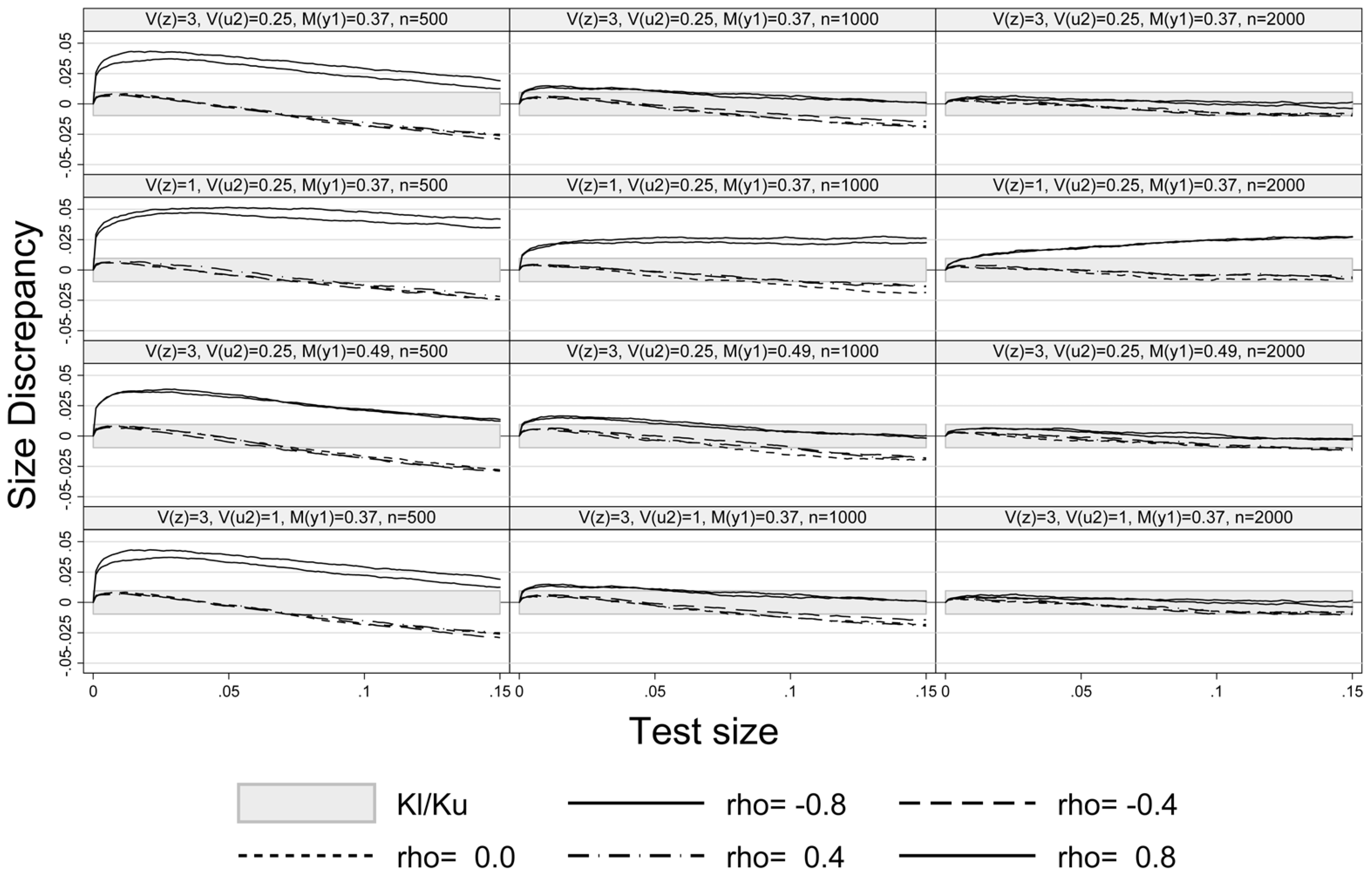
Figure 1 exhibits the size-discrepancy plots for Experiments 1–4 and sample sizes $n=500$, $1000,2000$. The plots show that the pseudo-score LM test is properly sized for $\rho =-0.4$ and $\rho =0.4$ in all experiments, while it slightly over-rejects at $\rho =-0.8$ and $\rho =0.8$, especially at a small sample size ($n=500$). For example, at a nominal test size of $0.05$ and a sample size of 1000 the size of LM test is too high by $0.012$ percentage points at $\left|\rho \right|=0.8$. For $\rho =-0.4$ and $\rho =0.4$ the size-discrepancy is within the Kolmogorov and Smirnov $5\%$ confidence of bound p ± $0.0096$ for p-values smaller than $0.1$. A similar result has also been mentioned in Montes-Rojas (2011) [9] in case of robust LM and $C\left(\alpha \right)$ tests. A weaker exclusion restriction, setting $Var\left(z_{1i}\right)=1/3$ in Experiment 2, increases the size-discrepancy at high absolute values of ρ (Experiment 2, row 2 of Figure 1), but hardly affects the size of the test at $\left|\rho \right|=0.4$. The size-discrepancy remains in the confidence bounds at medium values of ρ. Increasing the share of unobserved values to 0.49 (Experiment 3, row 3 of Figure 1) hardly affects the size-discrepancy. Lastly, Experiment 4 (last row of Figure 1) shows that a weaker fit ($Var\left(u_{2,i}\right)=1$) does not result in a larger size distortion as compared to the baseline in the first row of Figure 1. As one would expect, a larger number of observations generally enhances the performance of the LM test (see the last column in Figure 1). However, the large sample approximation improves relatively slowly with sample size under a weak exclusion restriction at high absolute values of ρ (confer the second row of graphs in Figure 1).

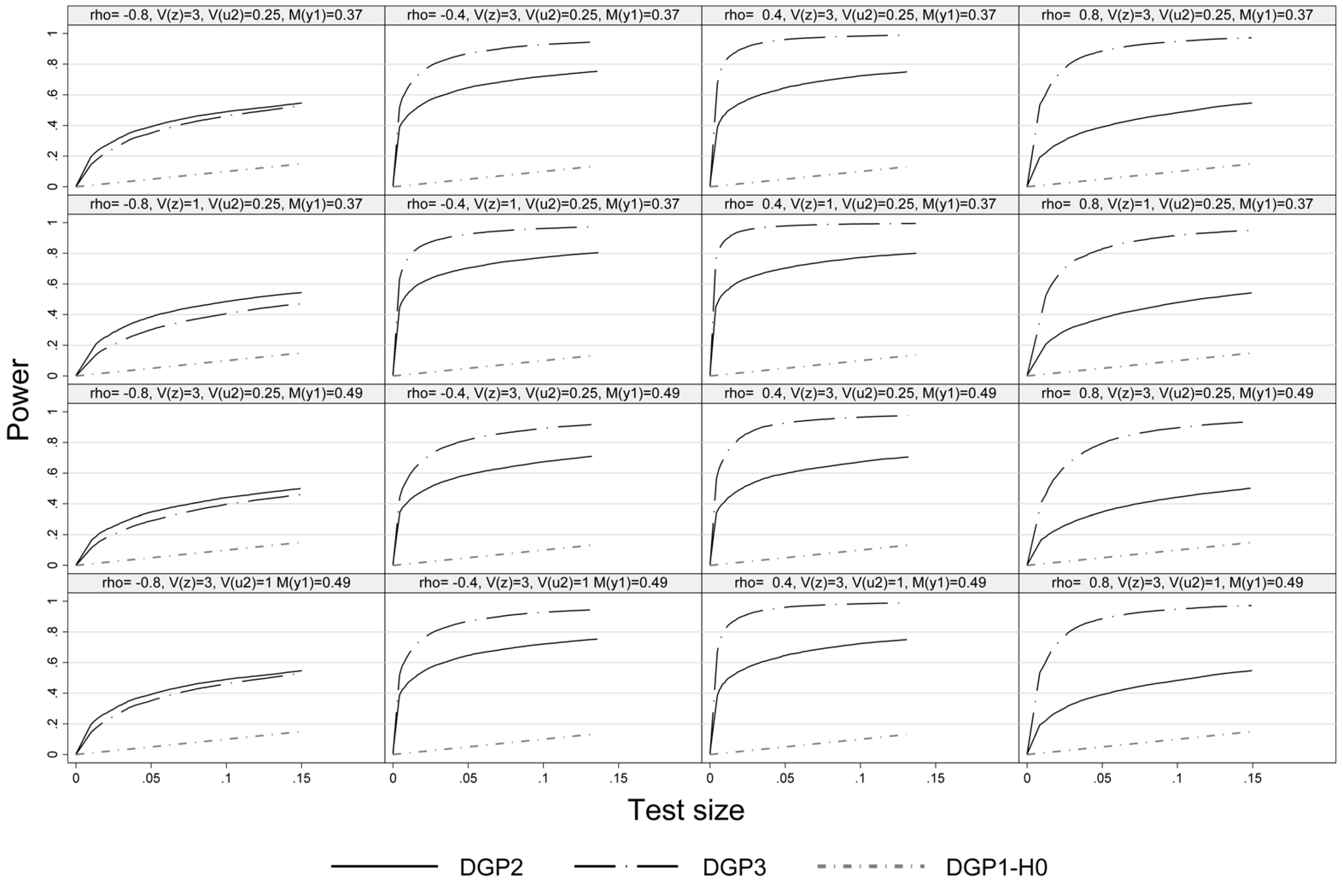
Figure 2, Figure 3 and Figure 4 present the power-size plots of the pseudo-score LM test for the DGPs 2–3, 4–5 and 6–7, respectively. In general and in line with the literature, for all DGPs referring to the alternative hypothesis we observe lower power of the pseudo-score LM test at high absolute values of ρ, but especially so at $\rho =-0.8$. If the distribution of the disturbances of the outcome equation exhibits both skewness and excess kurtosis (DGP3) the simulated power of the pseudo-score LM test is higher than that of a symmetric distribution with fatter tails than the normal distribution except for ($\rho =-0.8$). Furthermore, for DGP3 the power is generally lower at $\rho =-0.8$ as compared to large positive values ($\rho =0.8)$, which reflects differences in the skewness of the distribution of $u_{2i}$ with respect to ρ (confer Table 1).

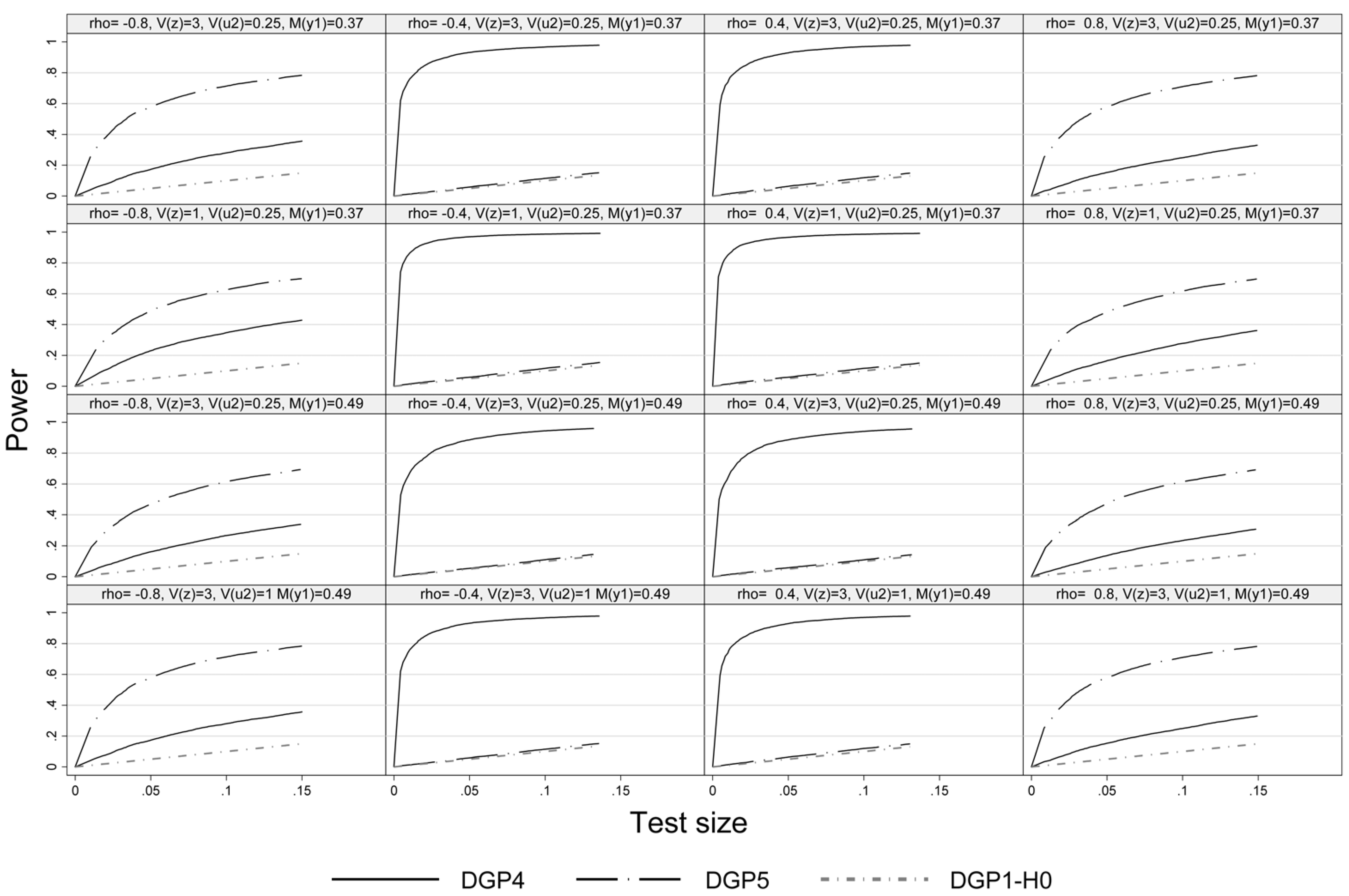
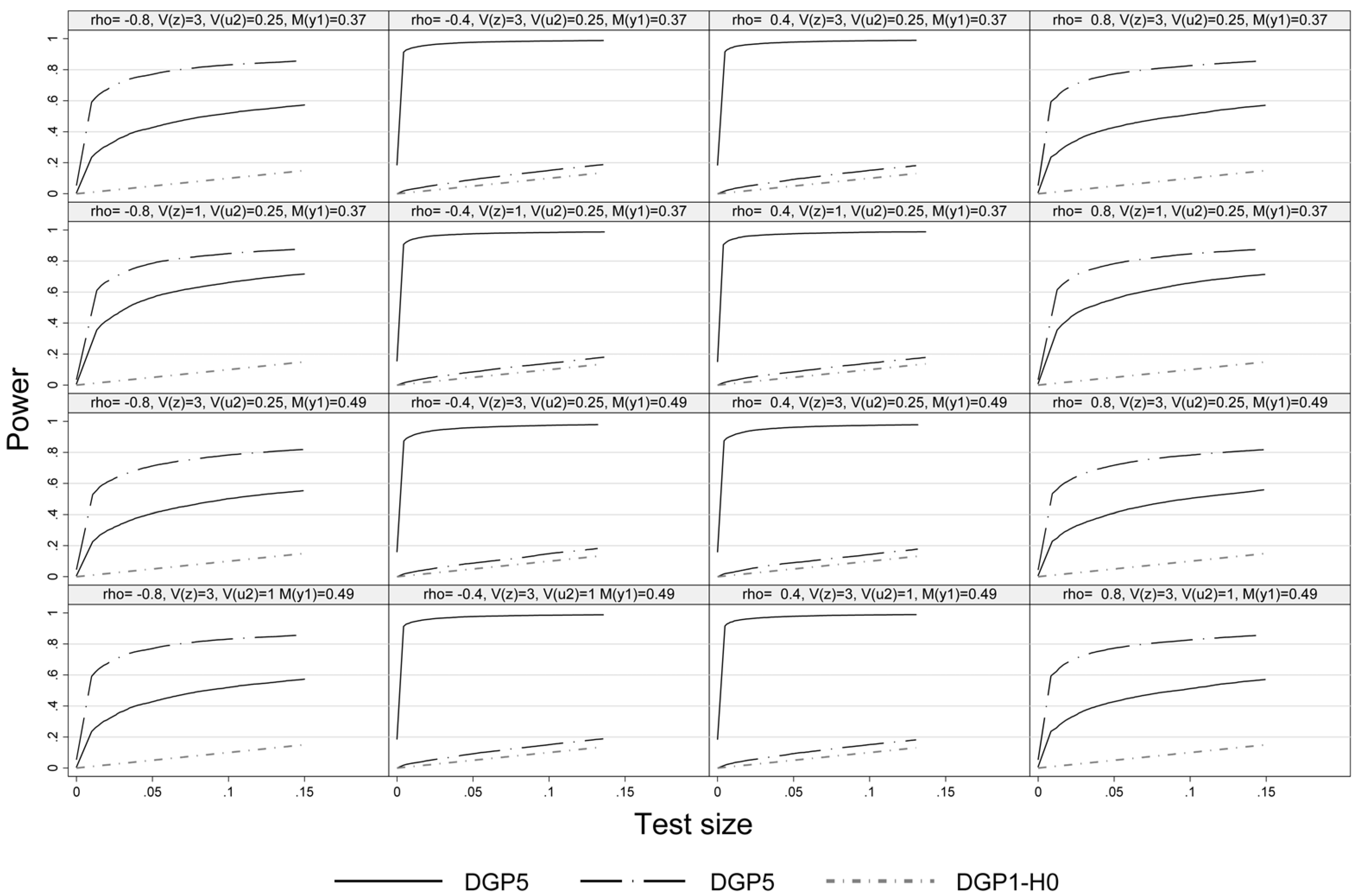
Figure 3 illustrates the power of the pseudo-score LM test under non-normality in either the outcome (DGP4) or the selection equation (DGP5) but not in both. Under DGP4 the pseudo-score LM test exhibits high power at intermediate absolute values of ρ, while at high absolute values of ρ the power tends to be lower as the weight of $u_{1i}$ (that is assumed to be normal) is higher in the disturbances of the outcome equation. In case of DGP5 we see the reversed pattern. Deviations from normality are only detected in case of high absolute values of ρ. Actually, under DGP5 the test has no power at all at $\rho =0$, since in this case there is no effect of the truncation of $u_{i1}$ and disturbances of the outcome equation are normal. This results can be found in all four considered Experiments.

Figure 4 presents the size-power plot of DGP6 and DGP7 and refers to heteroskedasticity. DGP6 allows for heteroskedasticity in the outcome equation and DGP7 in the selection equation. The power-size curves indicate that the pseudo-score LM test is also able to detect this type of deviation from the model assumptions as heteroskedasticity translates into pronounced excess kurtosis of the disturbances of the outcome equation. For DGP6 this is the case at medium to low values of $\left|\rho \right|$. DGP7 introduces heteroskedasticity in Probit selection model. In this case, the LM test exhibits power at high absolute vales of ρ, but has virtual no power at $\rho =-0.4$ and $0.4$. The reason is that the nominal kurtosis of $u_{2i}$ is hardly affected (amounting to 3.06, see Table 1) and the bias of the Mills’ ratio and the estimated coefficients of the outcome equation, especially that of the Mills’ ratio turn out small in comparison.

Figure 1. Size-discrepancy plot.

Figure 1. Size-discrepancy plot.

Figure 2. Size power plot, DGP1-DGP3, n = 1000.

Figure 2. Size power plot, DGP1-DGP3, n = 1000.

Figure 3. Size power plot, DGP1, DGP4 and DGP 5, n = 1000.

Figure 3. Size power plot, DGP1, DGP4 and DGP 5, n = 1000.

Figure 4. Size power plot, DGP1, DGP6 and DGP7, n = 1000.

Figure 4. Size power plot, DGP1, DGP6 and DGP7, n = 1000.

Comparing the first and second row of graphs in Figure 2, Figure 3 and Figure 4 indicates that there is not much power lost with the weaker exclusion restriction. A higher share of unobserved units tends to slightly reduce the power of the LM test as one would expect (see the graphs in row 3 vs. 1 in Figure 2, Figure 3 and Figure 4). Comparing the first and the last row in Figure 2, Figure 3 and Figure 4 indicates that a weaker fit (i.e., $Var\left(u_{2i}\right)$ is increased from 0.25 to 1) does not result in a significant loss of power. Lastly, as expected a larger sample size improves the power of the pseudo-score LM test across the board.4

4. Conclusions

Using Meijer and Wansbeek’s (2007) [10] GMM-approach for two-step estimators of the Heckman sample selection model, this paper introduces a pseudo-score LM test to check the assumption of normality and homoskedasticity of the disturbances, a prerequisite for the consistency of this estimator. The GMM-based pseudo-score LM test is easy to calculate and similar to the widely used Jarque and Bera (1980) [11] LM test. Indeed, in the absence of sample selection it reverts to their LM test statistic. In particular, the test checks whether the third and fourth moments of the disturbances of the outcome equation of the Heckman model conform to those implied by the truncated normal distribution. Under $H_0$ normal disturbances of the selection equation and the absence of heteroskedasticity in both the outcome and the selection equation are additionally required.

Monte Carlo simulations show good performance of the pseudo-score LM test for samples of size 1000 or larger and a powerful exclusion restriction. However, in line with other tests of the normality assumption of the Heckman sample selection model proposed in the literature the pseudo-score LM test tends to be oversized, although only slightly, if the correlation of the disturbances of the selection and the outcome equation is high in absolute value or if the exclusion restrictions are weak. Hence, this test can be recommended for sample sizes of 1000 or larger.