
On the Validity of Granger Causality for Ecological Count Time Series


1
Laboratory of Forest Economics, School of Forestry and Natural Environment, Aristotle University of Thessaloniki, 54124 Thessaloniki, Greece
2
Department of Electrical and Computer Engineering, Aristotle University of Thessaloniki, 54124 Thessaloniki, Greece
*
Author to whom correspondence should be addressed.
Econometrics 2024, 12(2), 13; https://doi.org/10.3390/econometrics12020013
Submission received: 22 February 2024
/
Revised: 28 April 2024
/
Accepted: 7 May 2024
/
Published: 9 May 2024
Abstract
:Knowledge of causal relationships is fundamental for understanding the dynamic mechanisms of ecological systems. To detect such relationships from multivariate time series, Granger causality, an idea first developed in econometrics, has been formulated in terms of vector autoregressive (VAR) models. Granger causality for count time series, often seen in ecology, has rarely been explored, and this may be due to the difficulty in estimating autoregressive models on multivariate count time series. The present research investigates the appropriateness of VAR-based Granger causality for ecological count time series by conducting a simulation study using several systems of different numbers of variables and time series lengths. VAR-based Granger causality for count time series (DVAR) seems to be estimated efficiently even for two counts in long time series. For all the studied time series lengths, DVAR for more than eight counts matches the Granger causality effects obtained by VAR on the continuous-valued time series well. The positive results, also in two ecological time series, suggest the use of VAR-based Granger causality for assessing causal relationships in real-world count time series even with few distinct integer values or many zeros.
1. Introduction
The methodology of linear analyses of univariate time series is widely known and applied frequently in several scientific disciplines, including ecology. Ecology, additionally, has provided some of the baseline material for nonlinear time series modeling (Tong 1977; Tong and Lim 1980). However, many problems in ecology (Jassby and Powell 1990; Turchin and Taylor 1992) as well as in other fields, e.g., economics (Mountford and Uhlig 2009), involve simultaneous observations of many quantities requiring methods of multivariate time series analysis (Lütkepohl 2005; Brandt and Williams 2007). The fundamental property one would first investigate in multivariate time series is the interdependence of the observed variables, formulated explicitly with the concept of Granger causality (Granger 1969).
Multivariate time series analysis, and Granger causality in particular, is mainly performed on multivariate time series of continuous-valued variables and relies, essentially, on vector autoregressive (VAR) models (Sims 1980). The causal relationship between two time series was first defined by Granger (1969) in econometrics and it was formulated as the improvement in the prediction of one variable when including in the prediction model the current and past values of another variable. In this case, it is said that the latter variable Granger-causes the former one, i.e., the current and past values of the one variable improve the prediction of the other variable. The strength of Granger causality is quantified with the Granger causality index (GCI), and the presence of Granger causality is decided by the Granger causality test (Brandt and Williams 2007).
In ecology, it is of great interest to find relationships in ecological systems and explain the causal effects among the involved variables (Bonan and Shugart 1989). However, Granger causality has not been used as frequently in ecology as in other environmental sciences (Detto et al. 2012; Gan 2006; Sugihara et al. 2012; Barraquand et al. 2020; Lam et al. 2023). This may be due to the lack of long and uninterrupted (without gaps) time series. On the other hand, VAR models, also called multivariate autoregressive models (MAR or MVAR), as well as state-space models, have been popular in ecology in describing complex ecological systems (Hampton et al. 2013; Auger-Méthé et al. 2021). However, the presence of a variable in the model does not directly establish a causal relationship of this variable to the response variable. Granger causality makes use of the VAR model to define this causal relationship explicitly. To be more precise, Granger causality is estimated using two VAR models: the unrestricted VAR model of all variables (U-model) and the restricted VAR model of all but the driving variable (R-model).
Ecological time series are often in the form of count data (Gerber and Kendall 2017), such as, for example, the number of an endangered species’ individuals in a wildlife refuge. This may be another reason why Granger causality has not been used much in ecology.
Analyses of count time series have been developed rather independently of the analysis of continuous-valued time series (Davis et al. 2021), as it is argued that the traditional methods for handling time series are not applicable to count data (Fokianos 2012; Fokianos et al. 2022). This is because, according to Tjøstheim (2012), in the standard time series setting, the condition for integer response and predictor variables, as well as integer coefficients and errors, would likely give rise to the non-stationarity of the underlying processes, an attribute one wants to avoid when modeling stationary time series.
Moreover, as suggested in O’Hara and Kotze (2010), count data should not be log-transformed (to stabilize the variance), especially when they contain zeros. In this respect, models developed for the analysis of continuous-valued time series have also been used in the analysis of ecological count time series, such as state space models (Newman et al. 2014; Hostetler and Chandler 2015) and generalized linear models (GLMs) (Zeger 1988). Although methods for analyzing univariate count time series with applications are present in the literature (McKenzie 1985; Al-Osh and Alzaid 1987; Park and Oh 1997; Barry and Welsh 2002; Cunningham and Lindenmayer 2005; Held et al. 2005; Ver Hoef and Boveng 2007; Richards 2008; Weiß 2008; Fokianos and Fried 2010; Lindén and Mäntyniemi 2011; Andersson and Karlis 2014; Ahmad and Francq 2016; Bourguignon et al. 2019; Kong and Lund 2023), the works on multivariate count time series analysis are disproportionately less (Fokianos 2021; Weiß 2021). The analysis of multivariate count time series regards distribution models, such as Poisson (Fokianos et al. 2009; Neumann 2011; Chan and Wan 2014; Piancastelli et al. 2023), binomial and negative binomial (Davis and Wu 2009; Scotto et al. 2014; Christou and Fokianos 2015), and autoregressive models (Franke and Rao 1993; Heinen and Rengifo 2007), such as Pegram’s autoregressive models (Song et al. 2013; Angers et al. 2017) and the multivariate integer-valued autoregressive (MINAR) models (Pedeli and Karlis 2011; Pedeli and Karlis 2013a, 2013b; Scotto et al. 2015; Santos et al. 2021). There are also other application-oriented approaches (Jung et al. 2011; Held et al. 2005; Paul et al. 2008; Paul and Held 2011), observation-driven models, and models based on Markov chains (Catania and Di Mari 2021; Fokianos et al. 2022).
The shortage of approaches for Granger causality for multivariate count time series, discussed by Shojaie and Fox (2022), is the motivation for the present study. In this work, we investigate the appropriateness of the widely used VAR models in estimating causal relationships in ecological multivariate time series of count data, typically being short and often involving only a few distinct integer values. We term the implementation of VAR on integer time series as a discrete VAR (DVAR) approach.
To address the appropriateness of DVAR, the aim of this study is to find the minimum range of count data for which DVAR models reliably identify the Granger causality. We conduct a simulation study using both continuous-valued and integer-valued systems derived by discretization, using a varying number of bins (integers). We also consider integer time series generated by the MINAR system. Further, we apply the DVAR approach to two ecological multivariate time series. The results of this study allow us to give guidelines for data collection in ecology and other disciplines.
The structure of this paper is as follows. In Section 2, we present VAR and Granger causality, as well as the simulated systems and the two ecological time series. In Section 3, we present the results of the simulations and their application in ecology, and in Section 4, the results are discussed. The final conclusions are then given in Section 5.
2. Materials and Methods
2.1. Vector Autoregressive Models and Granger Causality
A VAR(p) model to be fitted to time series data of K variables of length N, {yk,t}, k = 1, …, K and t = 1, …, T, is defined as follows (Lütkepohl 2005):
where v is the constant term vector of length K and Ai, i = 1, …, p are coefficient matrices of size K × K; yt is the vector of K variables in time t and et is the vector of K white noise input variables, with E(et) = 0 (0 is the K × 1 zero vector), and being diagonal, to exclude the presence of instantaneous Granger causality (Lütkepohl 2005), as is out of the scope of the current study.
The linear Granger causality is typically formulated in terms of VAR models; however, it is mentioned that many nonlinear Granger causality measures have been developed recently, such as information-based measures (Siggiridou et al. 2019). In the present study, we focus only on the linear Granger causality index (GCI) for bivariate time series and the conditional Granger causality index (CGCI) for multivariate time series (Geweke 1982), presented briefly below.
Let be the bivariate time series of two variables, X and Y. To investigate whether X Granger causes Y, denoted X → Y, two models for predicting Y are considered, the one containing past components of both X and Y, called unrestricted model (U-model), and the other excluding past components of X, called restricted model (R-model). Thus, the R-model is simply the autoregressive (AR) model for Y:
where p is the model order, αi is the model coefficients, and eR,t is the input white noise (assumed to be normally distributed), where the subscript ‘R’ denotes the R-model. The U-model adds to the form of the R-model the terms of past components of X for the same order p:
where eU,t is the input white noise of the U-model. The form in Equation (3) exemplifies the bivariate VAR(p) model in Equation (1) for Y. In the presence of Granger causality from X to Y, the fitting error in Equation (3) is expected to be smaller than the fitting error in Equation (2), and thus, the GCI is defined as follows (Geweke 1982):
where and are the estimated fitting errors of the R-model and the U-model, respectively. The GCI is close to zero when the variance of the two fitting errors is about the same and then X has no causal effect on Y, and it increases as the Granger causality from X to Y becomes stronger.
In the presence of other observed variables that may be correlated to any of X and Y, stacked in the vector variable Z, the conditional Granger causality from X to Y, denoted X → Y|Z, can be defined as the direct causality from variable X to variable Y, which is not mediated by another variable in Z. The corresponding conditional Granger causality index (CGCI) is similarly defined as
where and are the estimated fitting errors of the R-model and U-model defined as in Equation (2) and Equation (3), respectively, but both also including the p terms of lagged variables for each of the variables in Z.
In total, in a multivariate system of K observed variables, K×(K − 1) GCI and CGCI values can be calculated. The statistical significance of the GCI or CGCI for each causal effect X → Y is determined by the so-called Granger causality test, focusing on the statistical significance of all the coefficients of the lagged X variables in the U-model. The null hypothesis to be tested is H0: bi = 0 for i = 1, …, p. The parametric test is performed using the F statistic (Brandt and Williams 2007). In view of all pairs of the K variables, there are multiple tests on the same data, and typically, the criterion of false discovery rate (FDR) is called in to correct for multiple comparisons (Benjamini and Hochberg 1995).
The GCI and CGCI computations, as well as the respective Granger causality tests, are performed based on the VAR models fitted to the continuous-valued multivariate time series. We suggest the same analysis for Granger causality be applied to discrete-valued multivariate time series, i.e., count time series. Though the reasoning for the use of count data is that the variables can only make sense when they get integer values, this does not rule out the use of methods for continuous-valued data. The rationale is to treat the observed variables as being continuous-valued and attribute the integer values of the time series to round-off observational noise. Thus, the Granger analysis is applied to the count time series exactly as for the continuous-valued time series, and we refer to this as discrete VAR (DVAR) analysis, to stress that it is the standard VAR approach applied to discrete data.
To assess the overall accuracy of the VAR-based (DVAR-based when the data are assumed to be discrete) Granger causality, we consider the Matthews correlation coefficient (MCC) (Matthews 1975). Assigning as true positive (TP) and false negative (FN) the number of pairs of true Granger causality that were correctly found to be statistically significant and wrongly not found to be statistically significant, respectively, and true negative (TN) and false positive (FP) the number of pairs of not true Granger causality that were correctly not found to be statistically significant and wrongly found to be statistically significant, respectively, the MCC is defined as
where ‘’ denotes multiplication. The MCC can be seen as the correlation coefficient between the two true (or observed) classes (pairs having or not having Granger causality) and the two estimated (or predicted) classes, and it ranges between −1 and 1, with −1 meaning complete disagreement, 0 meaning random estimation (or prediction), and 1 meaning perfect match.
2.2. Simulations
In order to assess the validity of DVAR analysis and the accuracy of the derived GCI and CGCI, we perform extensive simulations in MATLAB (The MathWorks, Inc., Natick, MA, USA) on two continuous-valued VAR and three MINAR(1) systems, where the Granger causality relationships are known. The two VAR systems are as follows. (Supplementary Materials).
System 1: A VAR(5) system of four variables, a representative of the class of linear stochastic dynamic systems used in Winterhalder et al. (2005), defined as
x1,t = 0.8x1,t−1 + 0.65x2,t−4 + e1,t
x2,t = 0.6x2,t−1 + 0.6x4,t−5 + e2,t
x3,t = 0.5x3,t−3 − 0.6x1,t−1 + 0.4x2,t−4 + e3,t
x4,t = 1.2x4,t−1 − 0.7x4,t−2 + e4,t
There are four direct Granger causality relationships in a total of 12 pairs: i. X1→ X3, ii. X2 → X1, iii. X2 → X3, iv. X4 → X2.
System 2: A VAR(4) system of five variables, selected because it exhibits oscillating behavior and simulates cyclic-like activity. This system is used in Schelter et al. (2006) and it is defined as
x1,t = 0.4x1,t−1 − 0.5x1,t−2 + 0.4x5,t−1 + e1,t
x2,t = 0.4x2,t−1 − 0.3x1,t−4 + 0.4x5,t−2 + e2,t
x3,t = 0.5x3,t−1 − 0.7x3,t−2 − 0.3x5,t−3 + e3,t
x4,t = 0.8x4,t−3 + 0.4x1,t−2 + 0.3x2,t−3 + e4,t
x5,t = 0.7x5,t−1 − 0.5x5,t−2 − 0.4x4,t−1 + e5,t
This system has 7 direct Granger causality relationships in a total of 20 pairs: i. X1 → X2, ii. X1 → X4, iii. X2 → X4, iv. X4 → X5, v. X5 → X1, vi. X5 → X2, vii. X5 → X3.
An MINAR(1) system has the general form Xt = A o xt−1 + et, where Xt is the integer-valued vector variable of dimension K and et is the innovation vector of K (independent here) Poisson variables (we set the Poisson parameter equal to 0.1 in order to have a small range of integer values), A is a coefficient matrix of size K × K, and ‘o’ is the vector thinning operator (for details, see Franke and Rao (1993); Pedeli and Karlis (2013a); Boudreault and Charpentier (2011)). Below, we list three MINAR(1) systems we use in the simulations in 2, 3 and 4 variables, respectively.
System 3: An MINAR(1) system of two variables taking integer values from 0 up to 4 and 3, respectively, with the following coefficient matrix:
giving the relationship X2 → X1.
System 4: An MINAR(1) system of 3 variables taking integer values from 0 up to 6, 4 and 3, respectively, with the following coefficient matrix:
giving the following relationships: i. X2 → X1, ii.. X3 → X1, iii. X3 → X2.
System 5: An MINAR(1) system of 4 variables taking integer values from 0 up to 10, 6, 4 and 3, respectively, with the following coefficient matrix:
giving the following relationships: i. X2 → X1, ii. X3 → X1, iii. X3 → X2, iv. X4 → X1, v. X4 → X2, vi. X4 → X3.
To obtain statistically valid results, we consider 1000 realizations of each VAR and MINAR system and different lengths of the generated time series, namely, N = 50, 100, and 1000. For the three MINAR systems, we use also N = 25 because the systems are of order one, allowing estimation even for very short time series.
For the two VAR systems, the Granger causality is quantified by the GCI and CGCI on the original continuous-valued time series (VAR approach with p equal to the true order), serving as a reference for the DVAR approach. The statistical significance of the GCI and CGCI is tested with the F-statistic and the FDR for significance level a = 0.05. Then, the multivariate time series are discretized at varying ranges of integer values, and for each range, the GCI and CGCI are calculated on the count multivariate time series (DVAR with p equal to the true order). The varying range of count data is R = 2, 4, 6, 8, 10, 15, 20, 30, 40 and 60. Further, the accuracy of VAR and DVAR (for a different range of integer values) in matching the true Granger causality relationships of the system is assessed by the MCC.
2.3. Applications
Ecological time series, especially wildlife time series, are typically short. The first studied time series is for Common Eider (Somateria mollissima) (Milne 1965), available at the Global Population Dynamics Database of Imperial College (NERC Centre for Population Biology, Imperial College 2010; data reliability labeled as medium). The data (pop) are the monthly population abundance of the species as observed at the Ythan Valley of Aberdeenshire, Scotland, United Kingdom (descriptive statistics: min = 300, max = 3250, and median = 800 individuals). The time span is from February 1955 to February 1965 (N = 121) and includes 11 missing values.
The Granger causal effect of abiotic factors on the population of Common Eider is examined, where the time series of abiotic factors are obtained from the meteorological station in Nairn, Scotland (Met Office 2014). The monthly time series of the following five variables are considered: (i) mean daily maximum temperature (tmax), (ii) mean daily minimum temperature (tmin), (iii) days of air frost (af), (iv) total rainfall (rain), (v) total sunshine duration (sun). There are some missing values in four of these series, which are filled with linear interpolation. Figure 1 presents the history plots of the six completed time series, one of the Common Eider abundance, and five of the abiotic factors’ series.
As shown in Figure 1, all the time series exhibit annual seasonality, but there is no indication of a trend in any of the series. For each time series, the seasonality is removed by subtracting the average value for each month of the year. The order p of the VAR model to be fitted to the six time series is found using the Akaike information criterion (AIC), implemented for VAR models in MATLAB. Then, we compute the GCI and CGCI using VAR and DVAR for varying ranges R. Further, we search for the minimum R of the DVAR that best matches the Granger causal relationships estimated by the VAR model. This is evaluated with the MCC measure computed for the relationships found by VAR against those found by the DVAR model for the specific R.
The second real example is of a count time series of measles data, as opposed to the discretized time series in the previous example. Measles dynamics have been investigated recently in multivariate count data but at a large range of integer values (ranging from 0 to >1000). Here, we use weekly counts of new measles cases in the administrative region of Weser-Erms in Lower Saxony in Germany, analyzed in Held et al. (2005). The dataset is available in the Surveillance package for R (Salmon et al. 2016; Meyer et al. 2017), containing 15 time series at different locations within the region spanning 104 weeks (year 2001 and 2002). Five time series have up to 2 measles cases (Figure 2a), another five time series have from 3 to 6 cases (Figure 2b), and the remaining five time series have from 9 to 51 cases (Figure 2c).
3. Results
3.1. Simulations
We first present, in detail, for System 1 the greatest difference expected between standard VAR and the DVAR with only two integer values (values 0 and 1, R = 2) and with length N = 50. Table 1 shows that, for VAR and DVAR, the mean CGCI from 1000 realizations for the 12 variable pairs, and the number of realizations, the CGCI was found to be statistically significant using the FDR correction at the significance level a = 0.05. For such a short N, the VAR approach does not achieve the accurate identification of the four true Granger causality effects. On the other hand, the proportion of false positives is below the significance level (less than 50 of the 1000 realizations for pairs of no true causality) and the same holds for DVAR with R = 2. As expected, DVAR has less power in identifying the true direct Granger causality relationships.
The performance of the DVAR improves and tends to match the performance of the VAR approach as R increases and as N increases. The improvement with R is demonstrated in Figure 3 for N = 100 in the form of boxplots, where the boxplot for each pair of variables gives the distribution of the CGCI from the 1000 realizations. Thus, at each panel, the 12 boxplots correspond to the 12 ordered variable pairs (for the order see Table 1), with the true direct Granger causality relationships being indexed as 2, 3, 7 and 10. The panel for VAR is to be compared with the panels for DVAR with R increasing from 2 to 60.
For N = 100, the pattern of the 12 boxplots for VAR is well preserved for all but the DVAR with R = 2. For the latter, the boxplot for Χ2 →Χ3 is at the same level as for the pairs of no direct Granger causality, whereas the other three are distinctly higher (to be compared with Table 1 for N = 50). As R increases, all four boxplots corresponding to pairs of true Granger causality rise from the zero level, and already for R = 10 the distributions of the CGCI values match those of the VAR approach well. Even for R < 10, DVAR identifies all the causal and non-causal relationships correctly, except from the relationship Χ2 →Χ3, which is found statistically significant less often than with the VAR approach.
The overall performance of VAR and DVAR in identifying the true Granger causality structure of the system is quantified with the MCC shown in Figure 4 for System 1 and N = 50, 100 and 1000. For N = 50 and R = 2, DVAR gives MCC = 0.3 and increases monotonically and fast, with R converging to MCC = 0.76, the score of the VAR approach, and effectively approaching this value for R > 15. For N = 100, the VAR approach gives MCC = 0.96, and the MCC for DVAR starts from 0.76 for R = 2 and converges faster than for N = 50, approaching the 0.96 level already for R = 10. For the largest time series length (N = 1000), the DVAR for R = 2 gives MCC = 0.9, which is close to MCC = 0.98 for the VAR approach and this level is reached with R = 4. These results suggest that DVAR is as efficient as VAR even for a very small range of integers when the time series is long enough.
The results for System 2 are similar, as shown for the MCC in Figure 5. Here, the seven true direct Granger causality relationships are harder to identify even with VAR. However, the MCC of the DVAR converges with R to the MCC of VAR even faster than for System 1 and effectively obtains the same MCC for R > 8.
The same analysis on the basis of the GCI (assuming no conditioning on the other variables) showed the equivalent matching of DVAR to VAR depending, similarly, on R and N.
For the MINAR(1) systems of the number of variables K = 2, 3 and 4, the DVAR approach performed equally well as for the discretization of the continuous-valued time series and identified the true causal relationships. As seen in Table 2 and Figure 6, even for K = 2 and N = 25, the FDR-corrected Granger causality test identifies the true relationship, X2→X1, in 85% of the realizations. However, as the number of variables K increases, the H0 is rejected less times for N = 25 but in any case, the rate of false positives does not exceed the nominal level of 5%. DVAR has again the beneficial property of increasing the power of detecting the true causal relationships, with the increase in N reaching the maximum 100% often, even for N = 100.
3.2. Applications
In the first application of Common Eider data, the minimum AIC was found for p = 1, and we fit VAR(1) to the six time series. The estimation of the CGCI for all possible pairs resulted in the following two statistically significant direct Granger causal relationships: (i) tmax Granger causes tmin conditioning on the other four variables (CGCItmax->tmin = 0.0477, p = 0.02), and (ii) tmin Granger causes af conditioning on the other four variables (CGCItmin->af = 0.0588, p = 0.0098). Thus, the weather variables do not Granger-cause the Common Eider abundance. Note that, here, the statistical significance was not corrected with FDR for multiple testing; otherwise, no statistically significant Granger causality could be obtained. We discretized the system for R changing from 2 to 60 as in the simulations. For R = 2 and R = 4, DVAR failed to find the causal relationships indicated by VAR (another causal relationship was found for R = 4). This was succeeded first for R = 6 (but it still found another one). The plot of MCC for VAR and DVAR (for varying R), shown in Figure 7 (top panel), displays their match for R ≥ 8. The result that DVAR for R > 6 performs similarly to VAR is in agreement with the simulations.
We also examined the bivariate version of Granger causality (GCI). Usually, for such an ecological dataset, the researcher would be more interested in testing the causal effect of meteorological factors on the wild fauna species population (as it was, in this case, the Common Eider abundance). We concentrated on the causal relationship between a climatic variable and the Common Eider abundance. We searched at a higher-order p and found that, for p = 4 (minimum AIC), the days of air frost Granger-cause the Eider abundance. For this case, the VAR approach gave GCIaf->pop = 0.1077 with p = 0.0185. We discretized the two series for all R. As found previously, the DVAR with p = 4 succeeded in finding this causal relationship when R ≥ 6. The comparison of the GCI from VAR and DVAR for different R is shown in Figure 7 (bottom panel). It seems that the GCI from DVAR converges quickly with R to the GCI from VAR. In total, this application seems to support the findings of the simulations that DVAR is efficient in investigating Granger causality in ecological count data.
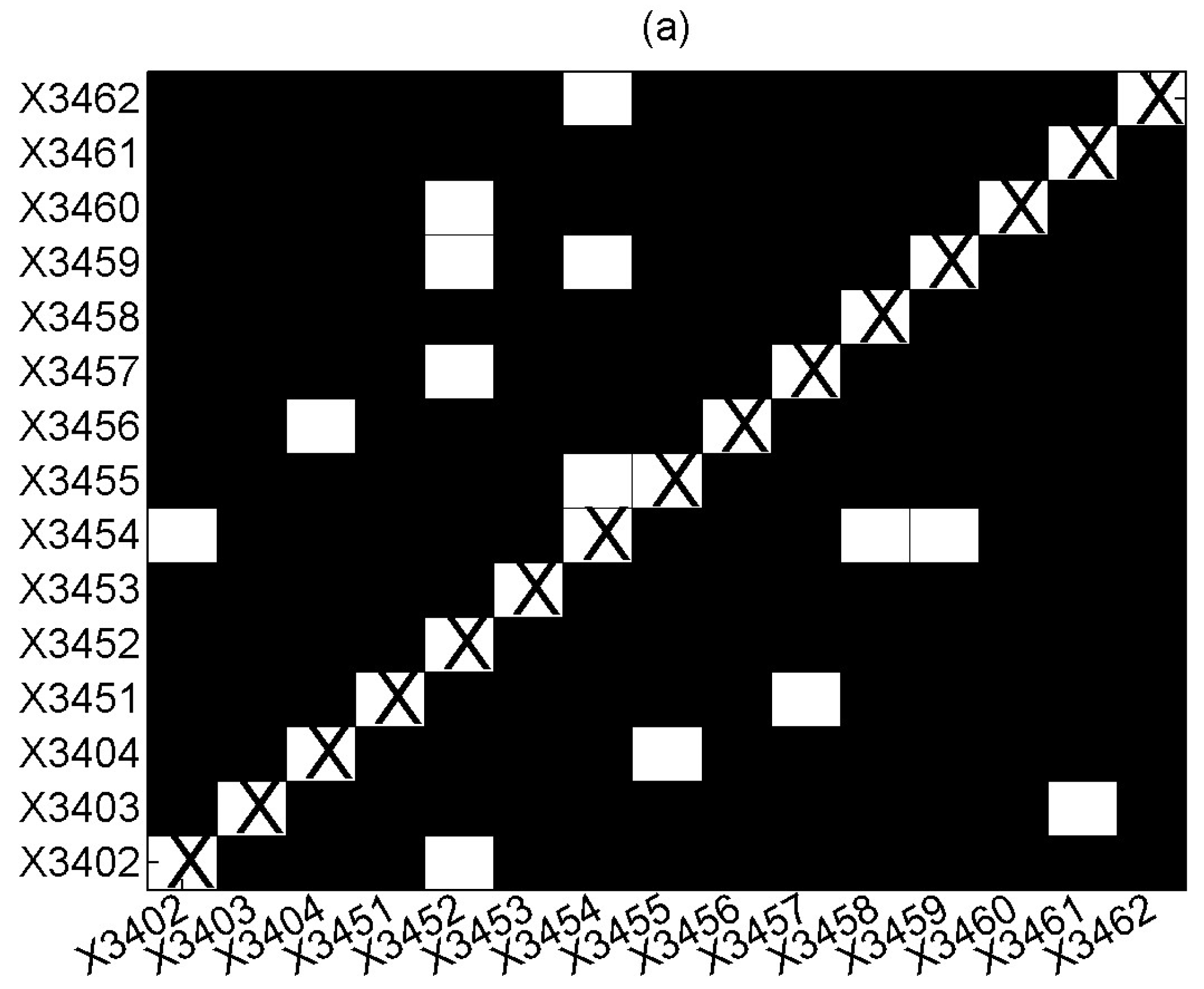
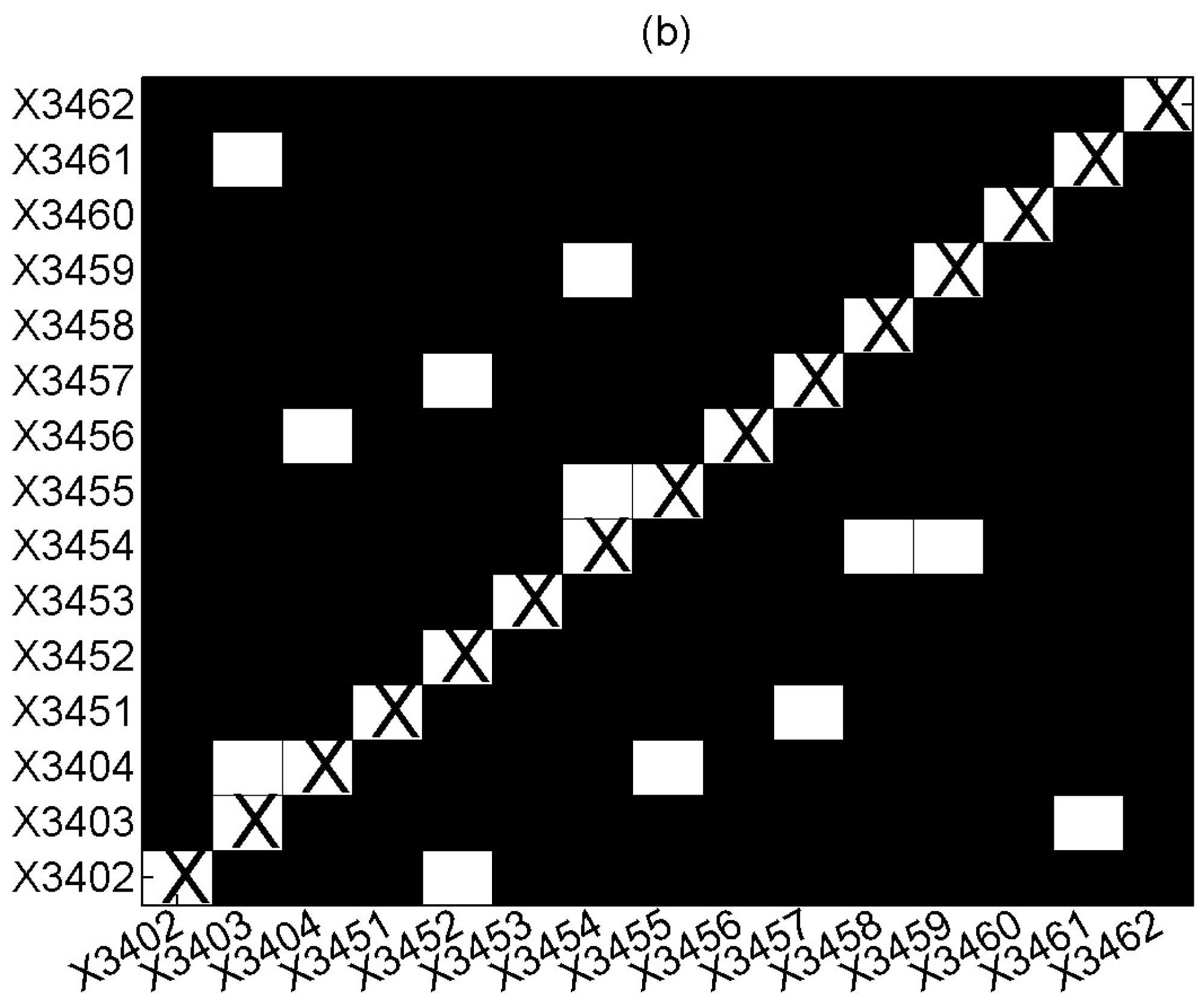
The second application on measles involves time series with very few integer values as well as fewer time series with large integer values. We applied DVAR (order p = 1) and the FDR correction for the significance of the CGCI at a = 0.05, where for each pair of locations, the dependence was computed conditioning on all other 13 locations. The results are shown in the form of a color matrix (white denotes statistically significant relationship, black no statistical significance) in Figure 8a. In Figure 8b, the same results are shown with the conditioning taken only on the neighboring locations, as these are specified in Meyer et al. (2017).
There is a good match between the detected Granger causality relationships: there are 14 significant relationships with conditioning on all locations and 10 of them are also significant when conditioning on the specified neighbors (out of 13). Though we cannot assess the validity of the positive (significant) and negative (non-significant) pair results, there seems to be a good agreement with the results of the CGCI based on DVAR when contrasting with the same results utilizing the information for the neighboring locations.
4. Discussion
4.1. Practical Implications
Count data are often encountered in ecological studies, and this study suggests the use of VAR models for finding Granger causality relationships in multivariate time series of count data. The simulations establish that VAR models can be an appropriate tool when dealing with count time series, a stand not previously supported in the literature (Fokianos et al. 2022).
Through our simulation study, it was found that for long discretized time series (N = 1000) generated by a VAR system, DVAR (VAR-based estimation of Granger causality on discrete-valued time series) efficiently identifies the causal and non-causal relationships even for the discretization of two integer values (0, 1). On the other hand, for very short count time series (N = 50), the correct identification requires a range of 10 integer values. The latter was confirmed also with simulations on time series generated by the multivariate count process MINAR(1). The power of DVAR in identifying causal relationships was good even for very short time series (N = 25), a useful finding for ecologists.
We applied DVAR to a set of short (N = 121) real ecological time series to investigate whether species abundance (Common Eider) is affected by abiotic variables. DVAR was found to estimate the same direct causal relationships as VAR when the discretized integer values were more than four. In all the simulations as well as the one application, rarely did we find false positive Granger causality relationships by DVAR that were not detected by VAR on the corresponding continuous-valued data. The second application on the weekly measles count data of a small integer range at 15 locations showed the good agreement of the causal relationships by DVAR when adding the information of neighboring locations.
Some practical guidelines arising from the present research may be helpful for scholars and practitioners working on ecological multivariate count time series:
- Tools of quantitative (numerical) analysis can indeed be applied to variables that take only a minimum of count values, for example 0, 1. For Granger causality, the shortcoming of having time series of few counts can be balanced by having long time series.
- Based on the latter result, it is suggested to rather use a small sampling time in the observation of ecological populations than aggregating the data in longer sampling times to produce bigger counts, and then use tools developed for continuous-valued data. Data aggregation, which is often the common practice, reduces the length of the time series and may have considerable effects (estimation accuracy, undetected seasonality or periodicity, occurrence of instantaneous causality). Indeed, it was shown in the simulation study that Granger causality is less accurately estimated with short time series.
- The present study suggests that the data precision can be relaxed at the cost of accuracy in the estimation of Granger causality. However, this cost can be compensated for by increasing the time series length, so that in the cases where high-quality data collection is difficult or costly, low-resolution observations may be adequate if the time series is long enough. For example, the abundance of the Common Eider species was rounded to hundreds of Eiders, and the same Granger causality relationships were estimated by counting the abundance in 10 classes of Eiders from 0 to 9 (0 for no Eiders). Some abiotic factors could easily be collected directly from the observers of Eiders, during their work, in similar classes. For instance, the temperature could have been classified in a scale from 0 to 9 (0 for temperatures close to the area’s minimum temperature for the season of observations).
We believe that the three previous practical guidelines suggest the broad use of Granger causality analysis in ecological systems. There are plenty of ecological multivariate count time series to which the proposed VAR model for Granger causality on count time series can be applied. Additionally, the strategies of data collection may be revised, also reducing the cost of field observations, and can even be applied to fields that were not previously possible to work on because of the low-quality and resolution of the observations.
4.2. Theoretical Implications
There are certain limitations and shortcomings of our approach, some of which could be addressed in future research. Though the selected applications confirmed the simulation study, more applications with real count time series are required to confirm whether the efficiency of DVAR is always the same. Additionally, future research should study the estimation of the strength of the Granger causality, as measured by the GCI and CGCI indexes. We did not work on this issue in depth, but we saw that in most of the cases, DVAR estimated a lower GCI and CGCI. It is possible that the GCI and CGCI computed by DVAR will converge to the respective indices computed by VAR in a wider range of counts than the range in which DVAR finds the same statistically significant causal relationships as VAR.
Nevertheless, more research and innovation are required in the field of analysis of multivariate count time series for the development of methods to reliably estimate the Granger causality among ecological (or other disciplines) count data. From our research, we have seen that the estimation of MINAR(1) models on multivariate count time series is a hard task, being currently under investigation by several researchers (Fokianos et al. 2022). In the works of Pedeli and Karlis (2011, 2013a), the estimation is restricted on diagonal forms (no interdependence among the different variables and no cross-correlation in the counts), and this is still the case in the periodic MINAR(1) extension of Santos et al. (2021). Additionally, in the work of Boudreault and Charpentier (2011), the general case considering both autocorrelation and cross-correlation is treated but the detailed estimation results are given only for the bivariate model, BINAR(1). The solution requires numerical optimization routines, and their use may be problematic for higher dimensions. We also note that the parameter estimation solution in the package Surveillance in R regards specific structures of the Poisson or negative binomial models (Paul and Held 2011). For the so-called vector Poisson regression (VPR) models and vector negative binomial regression (VNbR) models in Yip et al. (2013), details of the maximum likelihood estimation of the model parameters are not given.
A possible extension in the Granger causality analysis of count time series is the study of other measures of Granger causality, and in particular, information-based measures (e.g., see Siggiridou et al. (2019) for a survey simulation study), which can be directly applied to count data assuming the probability rather than density function of the involved variables (Papapetrou et al. 2022).
5. Conclusions
Granger causality for count time series is an underdeveloped topic in the statistics and econometrics literature. This has been one of the first attempts to show that the classical approach of Granger causality based on vector autoregressive (VAR) models designed for multivariate continuous-valued time series can also be applied to multivariate count time series. The VAR-based Granger causality on count time series seems to be estimated reliably even for two counts when the time series is long enough (a couple of hundreds in the simulations). For all the studied time series lengths, when there were more than eight counts, the estimation matched the Granger causality effects obtained by the VAR approach on the continuous-valued time series well. Policy implications may result from our analysis for several scientific disciplines such as economics and social and environmental sciences. The positive results suggest that researchers in ecology, as well as in other disciplines involving count data, use VAR-based Granger causality for assessing causal relationships in time series even with few distinct integer values, or many zeros in the count data.
Supplementary Materials
The following supporting information can be downloaded at https://www.mdpi.com/article/10.3390/econometrics12020013/s1.
Author Contributions
Conceptualization, K.G.P.; methodology, K.G.P. and D.K.; econometric analysis, K.G.P.; simulations, K.G.P. and D.K.; writing—original draft preparation, K.G.P.; writing—review and editing, D.K. All authors have read and agreed to the published version of the manuscript.
Funding
The authors acknowledge the Special Account for Research Funds of the Aristotle University of Thessaloniki, Greece, which funded the first author in the framework of the program Scholarships of Excellence for post-doctoral research (2013) under the supervision of the second author.
Institutional Review Board Statement
Not applicable.
Data Availability Statement
Data are available as a Supplementary File.
Conflicts of Interest
The authors declare no conflicts of interest.
References
- Ahmad, Ali, and Christian Francq. 2016. Poisson QMLE of Count Time Series Models. Journal of Time Series Analysis 37: 291–314. [Google Scholar] [CrossRef]
- Al-Osh, Mohamed A., and Aus A. Alzaid. 1987. First-Order Integer-Valued Autoregressive (INAR(1)) Process. Journal of Time Series Analysis 8: 261–75. [Google Scholar] [CrossRef]
- Andersson, Jonas, and Dimitris Karlis. 2014. A Parametric Time Series Model with Covariates for Integers in Z. Statistical Modelling 14: 135–56. [Google Scholar] [CrossRef]
- Angers, Jean-François, Atanu Biswas, and Raju Maiti. 2017. Bayesian Forecasting for Time Series of Categorical Data. Journal of Forecasting 36: 217–29. [Google Scholar] [CrossRef]
- Auger-Méthé, Marie, Ken Newman, Diana Cole, Fanny Empacher, Rowenna Gryba, Aaron A. King, Vianey Leos-Barajas, Joanna Mills Flemming, Anders Nielsen, Giovanni Petris, and et al. 2021. A Guide to State–Space Modeling of Ecological Time Series. Ecological Monographs 91: e01470. [Google Scholar] [CrossRef]
- Barraquand, Frédéric, Coralie Picoche, Matteo Detto, and Florian Hartig. 2020. Inferring Species Interactions Using Granger Causality and Convergent Cross Mapping. Theoretical Ecology 14: 87–105. [Google Scholar] [CrossRef]
- Barry, Simon C., and Alan H. Welsh. 2002. Generalized Additive Modelling and Zero Inflated Count Data. Ecological Modelling 157: 179–88. [Google Scholar] [CrossRef]
- Benjamini, Yoav, and Yosef Hochberg. 1995. Controlling the False Discovery Rate: A Practical and Powerful Approach to Multiple Testing. Journal of the Royal Statistical Society: Series B (Methodological) 57: 289–300. [Google Scholar] [CrossRef]
- Bonan, Gordon B., and Herman H. Shugart. 1989. Environmental Factors and Ecological Processes in Boreal Forests. Annual Review of Ecology and Systematics 20: 1–28. [Google Scholar] [CrossRef]
- Boudreault, Mathieu, and Arthur Charpentier. 2011. Multivariate Integer-Valued Autoregressive Models Applied to Earthquake Counts. arXiv arXiv:1112.0929. [Google Scholar]
- Bourguignon, Marcelo, Josemar Rodrigues, and Manoel Santos-Neto. 2019. Extended Poisson INAR(1) Processes with Equidispersion, Underdispersion and Overdispersion. Journal of Applied Statistics 46: 101–18. [Google Scholar] [CrossRef]
- Brandt, Patrick, and John Williams. 2007. Multiple Time Series Models. Thousand Oaks: Sage. [Google Scholar]
- Catania, Leopoldo, and Roberto Di Mari. 2021. Hierarchical Markov-Switching Models for Multivariate Integer-Valued Time-Series. Journal of Econometrics 221: 118–37. [Google Scholar] [CrossRef]
- Chan, Jennifer So Kuen, and Wai Yin Wan. 2014. Multivariate Generalized Poisson Geometric Process Model with Scale Mixtures of Normal Distributions. Journal of Multivariate Analysis 127: 72–87. [Google Scholar] [CrossRef]
- Christou, Vasiliki, and Konstantinos Fokianos. 2015. On Count Time Series Prediction. Journal of Statistical Computation and Simulation 85: 357–73. [Google Scholar] [CrossRef]
- Cunningham, Ross B., and David B. Lindenmayer. 2005. Modeling Count Data of Rare Species: Some Statistical Issues. Ecology 86: 1135–42. [Google Scholar] [CrossRef]
- Davis, Richard A., and Rongning Wu. 2009. A Negative Binomial Model for Time Series of Counts. Biometrika 96: 735–49. [Google Scholar] [CrossRef]
- Davis, Richard A., Konstantinos Fokianos, Scott H. Holan, Harry Joe, James Livsey, Robert Lund, Vladas Pipiras, and Nalini Ravishanker. 2021. Count Time Series: A Methodological Review. Journal of the American Statistical Association 116: 1533–47. [Google Scholar] [CrossRef]
- Detto, Matteo, Annalisa Molini, Gabriel Katul, Paul Stoy, Sari Palmroth, and Dennis Baldocchi. 2012. Causality and Persistence in Ecological Systems: A Nonparametric Spectral Granger Causality Approach. American Naturalist 179: 524–35. [Google Scholar] [CrossRef]
- Fokianos, Konstantinos. 2012. Count Time Series Models. In Handbook of Statistics. Amsterdam: Elsevier, vol. 30, pp. 315–47. [Google Scholar]
- Fokianos, Konstantinos. 2021. Multivariate Count Time Series Modelling. Econometrics and Statistics, in press. [Google Scholar] [CrossRef]
- Fokianos, Konstantinos, Anders Rahbek, and Dag Tjøstheim. 2009. Poisson Autoregression. Journal of the American Statistical Association 104: 1430–39. [Google Scholar] [CrossRef]
- Fokianos, Konstantinos, and Roland Fried. 2010. Interventions in INGARCH Processes. Journal of Time Series Analysis 31: 210–25. [Google Scholar] [CrossRef]
- Fokianos, Konstantinos, Roland Fried, Yuriy Kharin, and Valeriy Voloshko. 2022. Statistical Analysis of Multivariate Discrete-Valued Time Series. Journal of Multivariate Analysis 188: 104805. [Google Scholar] [CrossRef]
- Franke, Jürgen, and T. Subba Rao. 1993. Multivariate First Order Integer Valued Autoregressions. Berichte Der Arbeitsgruppe Technomathematik. Kaiserslaute: Universitgt Kaiserslautern, Fachbereich Mathematik. [Google Scholar]
- Gan, Jianbang. 2006. Causasilty among Wildfire, ENSO, Timber Harvest, and Urban Sprawl: The Vector Autoregression Approach. Ecological Modelling 191: 304–14. [Google Scholar] [CrossRef]
- Gerber, Brian D., and William L. Kendall. 2017. Evaluating and Improving Count-Based Population Inference: A Case Study from 31 Years of Monitoring Sandhill Cranes. The Condor 119: 191–206. [Google Scholar] [CrossRef]
- Geweke, John. 1982. Measurement of Linear Dependence and Feedback Between Multiple Time Series. Journal of the American Statistical Association 77: 304–13. [Google Scholar] [CrossRef]
- Granger, Clive W. J. 1969. Investigating Causal Relations by Econometric Models and Cross-Spectral Methods. Econometrica 37: 424–38. [Google Scholar] [CrossRef]
- Hampton, Stephanie E., Elizabeth E. Holmes, Lindsay P. Scheef, Mark D. Scheuerell, Stephen L. Katz, Daniel E. Pendleton, and Eric J. Ward. 2013. Quantifying Effects of Abiotic and Biotic Drivers on Community Dynamics with Multivariate Autoregressive (MAR) Models. Ecology 94: 2663–69. [Google Scholar] [CrossRef] [PubMed]
- Heinen, Andreas, and Erick Rengifo. 2007. Multivariate Autoregressive Modeling of Time Series Count Data Using Copulas. Journal of Empirical Finance 14: 564–83. [Google Scholar] [CrossRef]
- Held, Leonhard, Michael Höhle, and Mathias Hofmann. 2005. A Statistical Framework for the Analysis of Multivariate Infectious Disease Surveillance Counts. Statistical Modelling 5: 187–99. [Google Scholar] [CrossRef]
- Hostetler, Jeffrey A., and Richard B. Chandler. 2015. Improved State-Space Models for Inference about Spatial and Temporal Variation in Abundance from Count Data. Ecology 96: 1713–23. [Google Scholar] [CrossRef]
- Jassby, Alan D., and Thomas M. Powell. 1990. Detecting Changes in Ecological Time Series. Ecology 71: 2044–52. [Google Scholar] [CrossRef]
- Jung, Robert C., Roman Liesenfeld, and Jean-François Richard. 2011. Dynamic Factor Models for Multivariate Count Data: An Application to Stock-Market Trading Activity. Journal of Business & Economic Statistics 29: 73–85. [Google Scholar]
- Kong, Jiajie, and Robert Lund. 2023. Seasonal Count Time Series. Journal of Time Series Analysis 44: 93–124. [Google Scholar] [CrossRef]
- Lam, Weng Siew, Weng Hoe Lam, Saiful Hafizah Jaaman, and Pei Fun Lee. 2023. Bibliometric Analysis of Granger Causality Studies. Entropy 25: 632. [Google Scholar] [CrossRef]
- Lindén, Andreas, and Samu Mäntyniemi. 2011. Using the Negative Binomial Distribution to Model Overdispersion in Ecological Count Data. Ecology 92: 1414–21. [Google Scholar] [CrossRef]
- Lütkepohl, Helmut. 2005. New Introduction to Multiple Time Series Analysis. Berlin and Heidelberg: Springer. [Google Scholar]
- Matthews, Brian W. 1975. Comparison of the Predicted and Observed Secondary Structure of T4 Phage Lysozyme. Biochimica et Biophysica Acta (BBA)-Protein Structure 405: 442–51. [Google Scholar] [CrossRef]
- McKenzie, Ed. 1985. Some Simple Models for Discrete Variate Time Series. JAWRA Journal of the American Water Resources Association 21: 645–50. [Google Scholar] [CrossRef]
- Met Office, UK. 2014. Historic Station Data: Nairn. Available online: http://www.metoffice.gov.uk/pub/data/weather/uk/climate/stationdata/nairndata.txt (accessed on 16 July 2014).
- Meyer, Sebastian, Leonhard Held, and Michael Höhle. 2017. Spatio-Temporal Analysis of Epidemic Phenomena Using the R Package Surveillance. Journal of Statistical Software 77: 1–55. [Google Scholar] [CrossRef]
- Milne, H. 1965. Seasonal Movements and Distribution of Eiders in Northeast Scotland. Bird Study 12: 170–80. [Google Scholar] [CrossRef]
- Mountford, Andrew, and Harald Uhlig. 2009. What Are the Effects of Fiscal Policy Shocks? Journal of Applied Econometrics 24: 960–92. [Google Scholar] [CrossRef]
- NERC Centre for Population Biology, Imperial College. 2010. The Global Population Dynamics Database Version 2. Available online: http://www.sw.ic.ac.uk/cpb/cpb/gpdd.html (accessed on 16 July 2014).
- Neumann, Michael H. 2011. Absolute Regularity and Ergodicity of Poisson Count Processes. Bernoulli 17: 1268–84. [Google Scholar] [CrossRef]
- Newman, Ken, Stephen Terrence Buckland, Byron Morgan, Ruth King, David Louis Borchers, Diana Cole, Panagiotis Besbeas, Olivier Gimenez, and Len Thomas. 2014. Modelling Population Dynamics: Model Formulation, Fitting and Assessment Using State-Space Methods. Methods in Statistical Ecology. New York: Springer. [Google Scholar]
- O’Hara, Robert, and Johan Kotze. 2010. Do Not Log-transform Count Data. Methods in Ecology and Evolution 1: 118–22. [Google Scholar] [CrossRef]
- Papapetrou, Maria, Elsa Siggiridou, and Dimitris Kugiumtzis. 2022. Adaptation of Partial Mutual Information from Mixed Embedding to Discrete-Valued Time Series. Entropy 24: 1505. [Google Scholar] [CrossRef] [PubMed]
- Park, YouSung, and Chan Wook Oh. 1997. Some Asymptotic Properties in INAR(1) Processes with Poisson Marginals. Statistical Papers 38: 287–302. [Google Scholar] [CrossRef]
- Paul, Michaela, and Leonhard Held. 2011. Predictive Assessment of a Non-Linear Random Effects Model for Multivariate Time Series of Infectious Disease Counts. Statistics in Medicine 30: 1118–36. [Google Scholar] [CrossRef]
- Paul, Michaela, Leonhard Held, and André M. Toschke. 2008. Multivariate Modelling of Infectious Disease Surveillance Data. Statistics in Medicine 27: 6250–67. [Google Scholar] [CrossRef] [PubMed]
- Pedeli, Xanthi, and Dimitris Karlis. 2011. A Bivariate INAR(1) Process with Application. Statistical Modelling 11: 325–49. [Google Scholar] [CrossRef]
- Pedeli, Xanthi, and Dimitris Karlis. 2013a. On Composite Likelihood Estimation of a Multivariate INAR(1) Model. Journal of Time Series Analysis 34: 206–20. [Google Scholar] [CrossRef]
- Pedeli, Xanthi, and Dimitris Karlis. 2013b. Some Properties of Multivariate INAR(1) Processes. Computational Statistics & Data Analysis 67: 213–25. [Google Scholar]
- Piancastelli, Luiza S. C., Wagner Barreto-Souza, and Hernando Ombao. 2023. Flexible Bivariate INGARCH Process with a Broad Range of Contemporaneous Correlation. Journal of Time Series Analysis 44: 206–22. [Google Scholar] [CrossRef]
- Richards, Shane A. 2008. Dealing with Overdispersed Count Data in Applied Ecology. Journal of Applied Ecology 45: 218–27. [Google Scholar] [CrossRef]
- Salmon, Maëlle, Dirk Schumacher, and Michael Höhle. 2016. Monitoring Count Time Series in R: Aberration Detection in Public Health Surveillance. Journal of Statistical Software 70: 1–35. [Google Scholar] [CrossRef]
- Santos, Cláudia, Isabel Pereira, and Manuel Scotto. 2021. On the Theory of Periodic Multivariate INAR Processes. Statistical Papers 62: 1291–348. [Google Scholar] [CrossRef]
- Schelter, Björn, Matthias Winterhalder, Bernhard Hellwig, Brigitte Guschlbauer, Carl Hermann Lücking, and Jens Timmer. 2006. Direct or indirect? Graphical models for neural oscillators. Journal of Physiology-Paris 99: 37–46. [Google Scholar] [CrossRef]
- Scotto, Manuel G., Christian H. Weiß, and Sónia Gouveia. 2015. Thinning-Based Models in the Analysis of Integer-Valued Time Series: A Review. Statistical Modelling 15: 590–618. [Google Scholar] [CrossRef]
- Scotto, Manuel G., Christian H. Weiß, Maria Eduarda Silva, and Isabel Pereira. 2014. Bivariate Binomial Autoregressive Models. Journal of Multivariate Analysis 125: 233–51. [Google Scholar] [CrossRef]
- Shojaie, Ali, and Emily B. Fox. 2022. Granger Causality: A Review and Recent Advances. Annual Review of Statistics and Its Application 9: 289–319. [Google Scholar] [CrossRef] [PubMed]
- Siggiridou, Elsa, Christos Koutlis, Alkiviadis Tsimpiris, and Dimitris Kugiumtzis. 2019. Evaluation of Granger Causality Measures for Constructing Networks from Multivariate Time Series. Entropy 21: 1080. [Google Scholar] [CrossRef]
- Sims, Christopher A. 1980. Macroeconomics and Reality. Econometrica 48: 1–48. [Google Scholar] [CrossRef]
- Song, Peter X.-K., R. Keith Freeland, Atanu Biswas, and Shulin Zhang. 2013. Statistical Analysis of Discrete-Valued Time Series Using Categorical ARMA Models. Computational Statistics & Data Analysis 57: 112–24. [Google Scholar]
- Sugihara, George, Robert May, Hao Ye, Chih-hao Hsieh, Ethan Deyle, Michael Fogarty, and Stephan Munch. 2012. Detecting Causality in Complex Ecosystems. Science 338: 496–500. [Google Scholar] [CrossRef]
- Tjøstheim, Dag. 2012. Some Recent Theory for Autoregressive Count Time Series. TEST: An Official Journal of the Spanish Society of Statistics and Operations Research 21: 413–38. [Google Scholar] [CrossRef]
- Tong, Howell. 1977. Some Comments on the Canadian Lynx Data. Journal of the Royal Statistical Society: Series A (General) 140: 432–36. [Google Scholar] [CrossRef]
- Tong, Howell, and Keng S. Lim. 1980. Threshold Autoregression, Limit Cycles and Cyclical Data. Journal of the Royal Statistical Society: Series B (Methodological) 42: 245–68. [Google Scholar] [CrossRef]
- Turchin, Peter, and Andrew D. Taylor. 1992. Complex Dynamics in Ecological Time Series. Ecology 73: 289–305. [Google Scholar] [CrossRef]
- Ver Hoef, Jay M., and Peter L. Boveng. 2007. Quasi-Poisson vs. Negative Binomial Regression: How Should We Model Overdispersed Count Data? Ecology 88: 2766–72. [Google Scholar] [CrossRef] [PubMed]
- Weiß, Christian H. 2008. Serial Dependence and Regression of Poisson INARMA Models. Journal of Statistical Planning and Inference 138: 2975–90. [Google Scholar] [CrossRef]
- Weiß, Christian H. 2021. Stationary Count Time Series Models. WIREs Computational Statistics 13: e1502. [Google Scholar] [CrossRef]
- Winterhalder, Matthias, Björn Schelter, Wolfram Hesse, Karin Schwab, Lutz Leistritz, Daniel Klan, Reinhard Bauer, Jens Timmer, and Herbert Witte. 2005. Comparison of Linear Signal Processing Techniques to Infer Directed Interactions in Multivariate Neural Systems. Signal Processing 85: 2137–60. [Google Scholar] [CrossRef]
- Yip, Paul S. F., Simon Sai Man Kwok, Feng Chen, Xiaochen Xu, and Ying-Yeh Chen. 2013. A Study on the Mutual Causation of Suicide Reporting and Suicide Incidences. Journal of Affective Disorders 148: 98–103. [Google Scholar] [CrossRef]
- Zeger, Scott L. 1988. A Regression Model for Time Series of Counts. Biometrika 75: 621–29. [Google Scholar] [CrossRef]
Figure 1.
History plots of the Common Eider population and the five abiotic factor variables of the application.
Figure 1.
History plots of the Common Eider population and the five abiotic factor variables of the application.
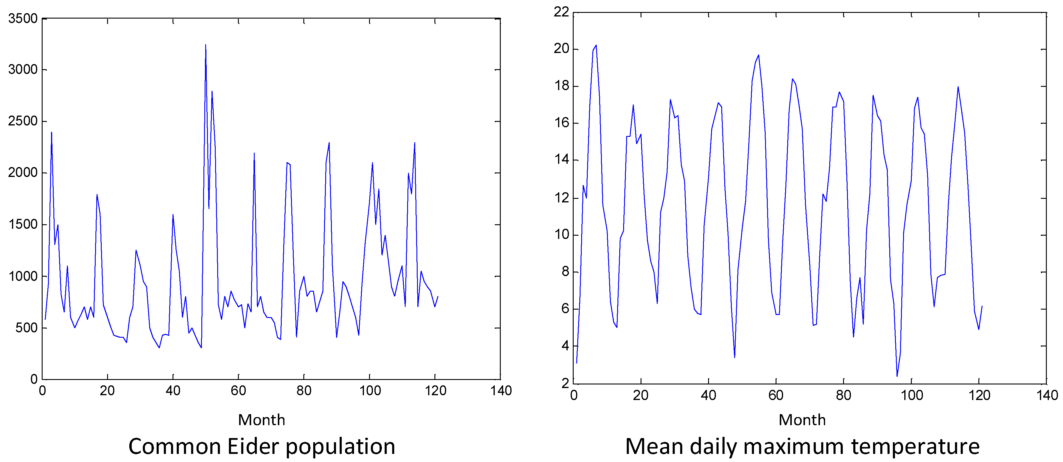

Figure 2.
The 15 time series of the weekly measles cases grouped according to the range of count data (up to 2 in (a), from 3 to 6 in (b), and from 9 to 51 in (c)), each time series labeled with the location code.
Figure 2.
The 15 time series of the weekly measles cases grouped according to the range of count data (up to 2 in (a), from 3 to 6 in (b), and from 9 to 51 in (c)), each time series labeled with the location code.
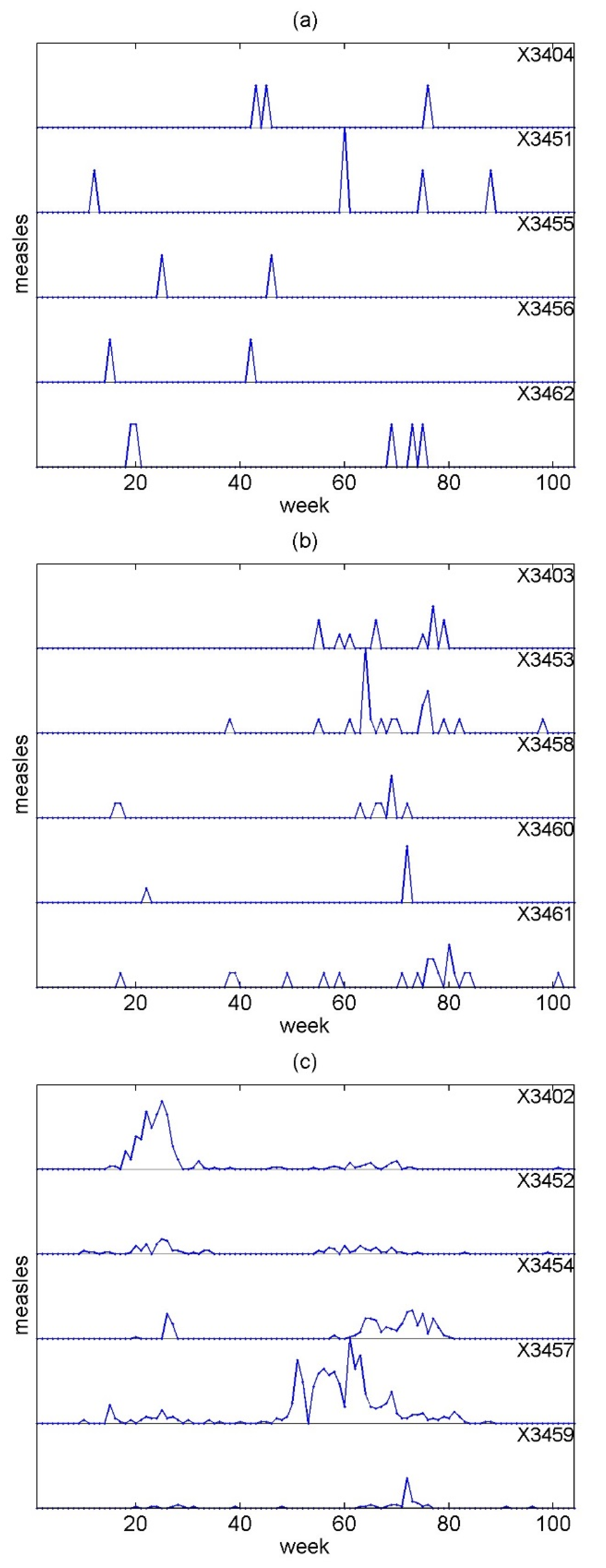
Figure 3.
Boxplot panels of the CGCI for the 12 variable pairs from 1000 realizations of System 1 for N = 100, where the left panel (labeled “VAR”) is for the VAR approach and the other panels are for the DVAR approach with varying range of integer values R.
Figure 3.
Boxplot panels of the CGCI for the 12 variable pairs from 1000 realizations of System 1 for N = 100, where the left panel (labeled “VAR”) is for the VAR approach and the other panels are for the DVAR approach with varying range of integer values R.

Figure 4.
MCC for the 12 true and estimated causal relationships by the CGCI using the VAR approach (bar) and the DVAR approach (curve) for varying R (x-axis) for System 1 and for N = 50 in (a), N = 100 in (b) and N = 1000 in (c).
Figure 4.
MCC for the 12 true and estimated causal relationships by the CGCI using the VAR approach (bar) and the DVAR approach (curve) for varying R (x-axis) for System 1 and for N = 50 in (a), N = 100 in (b) and N = 1000 in (c).

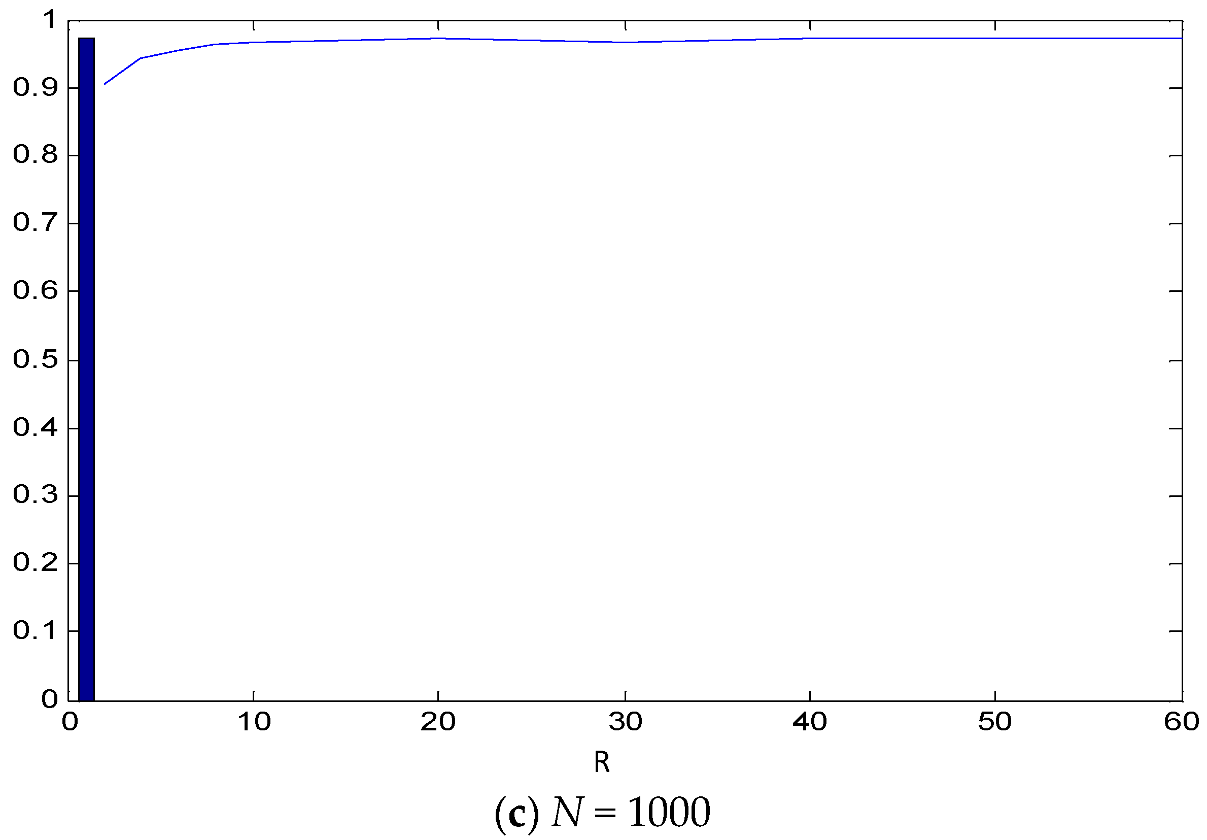
Figure 5.
MCC between true and estimated causal relationships by the CGCI using the VAR approach (bar) and the DVAR approach (curve) for varying R (x-axis) for System 2 and for N = 50 in (a), N = 100 in (b) and N = 1000 in (c).
Figure 5.
MCC between true and estimated causal relationships by the CGCI using the VAR approach (bar) and the DVAR approach (curve) for varying R (x-axis) for System 2 and for N = 50 in (a), N = 100 in (b) and N = 1000 in (c).
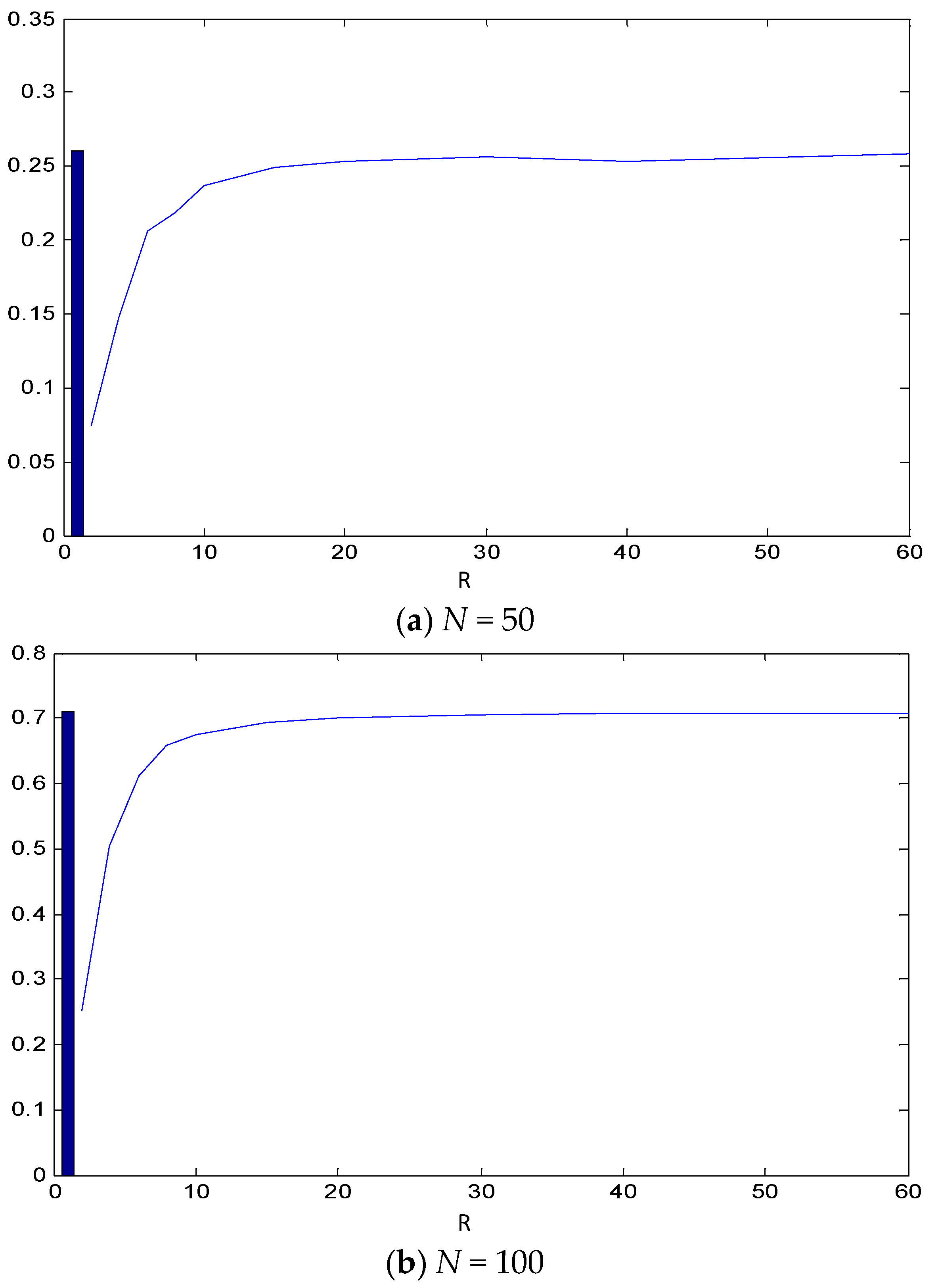

Figure 6.
Boxplot panels of the CGCI from DVAR on 1000 realizations of the MINAR(1) systems, System 3 in the left column, System 4 in the middle column and System 5 in the right column, and for N = 25, 50, 100, 1000, for the panels from top to bottom.
Figure 6.
Boxplot panels of the CGCI from DVAR on 1000 realizations of the MINAR(1) systems, System 3 in the left column, System 4 in the middle column and System 5 in the right column, and for N = 25, 50, 100, 1000, for the panels from top to bottom.
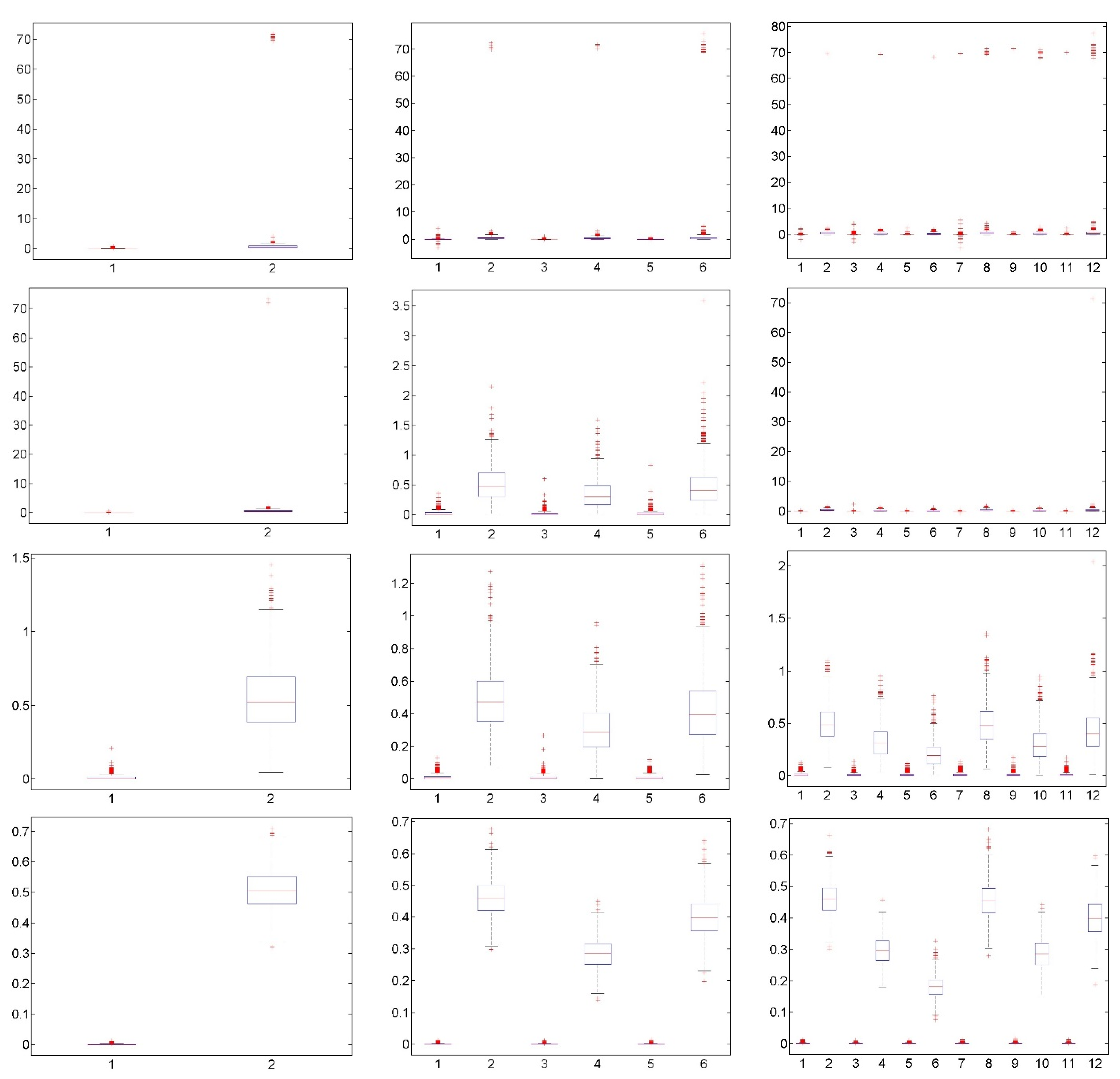
Figure 7.
Top panel: MCC for the Granger causal relationships estimated by the CGCI from the VAR approach and the DVAR approach for varying R (x-axis) considering all six ecological time series. Bottom panel: the GCI for the VAR approach (bar) and the DVAR approach (curve) for varying R (x-axis) for the Granger causality from air frost to Eider abundance.

Figure 8.
Black–white matrix for the statistical significance of CGCI (white: significant, black: not significant) on all pairs of the 15 time series of different locations of the measles dataset, where in (a), all 13 of the other locations (other than driving and response location of each pair) are included in the VAR model, and in (b), only the neighboring locations are included in the VAR model (X34nn is the number of the district).

Table 1.
Comparison of the VAR approach and the DVAR approach with R = 2 for System 1 and Ν = 50. The rows in bold show the pairs of true causal relationships; the arrow shows the direction of the relationship. The columns titled CGCI (for VAR and DVAR) display the mean CGCI in the 1000 realizations and the columns titled FDR (for VAR and DVAR) display the number of times the CGCI is found to be statistically significant at the significance level a = 0.05 using the FDR correction for multiple testing.
| Pair | CGCI (VAR) | FDR (VAR) | CGCI (DVAR) | FDR (DVAR) |
|---|---|---|---|---|
| X1 → X2 | 0.1906 | 18 | 0.1848 | 19 |
| X2 → X1 | 0.8900 | 890 | 0.3924 | 118 |
| X1 → X3 | 0.7560 | 781 | 1.0750 | 320 |
| X3 → X1 | 0.1922 | 16 | 0.1762 | 11 |
| X1 → X4 | 0.1847 | 19 | 0.1859 | 10 |
| X4 → X1 | 0.1868 | 17 | 0.1988 | 9 |
| X2 → X3 | 0.5097 | 419 | 0.1974 | 15 |
| X3 → X2 | 0.1885 | 20 | 0.1964 | 12 |
| X2 → X4 | 0.1925 | 18 | 0.1927 | 8 |
| X4 → X2 | 0.7879 | 830 | 0.3985 | 140 |
| X3 → X4 | 0.1864 | 25 | 0.1932 | 13 |
| X4 → X3 | 0.1905 | 18 | 0.1916 | 14 |
Table 2.
The average of GCI (for K = 2) and CGCI (for K > 2) from 1000 realizations of the MINAR(1) systems for K = 2, 3 and 4 (Systems 3 to 5) and the number of rejections of H0 with the FDR statistic. The true causal relationships are highlighted.
Table 2.
The average of GCI (for K = 2) and CGCI (for K > 2) from 1000 realizations of the MINAR(1) systems for K = 2, 3 and 4 (Systems 3 to 5) and the number of rejections of H0 with the FDR statistic. The true causal relationships are highlighted.
| K = 2 | N = 25 | N = 50 | N = 100 | N = 1000 | ||||
| Relation | GCI | FDR | GCI | FDR | GCI | FDR | GCI | FDR |
| X1 → X2 | 0.051 | 55 | 0.024 | 49 | 0.012 | 65 | 0.001 | 80 |
| X2→ X1 | 2.580 | 850 | 0.740 | 973 | 0.552 | 998 | 0.508 | 1000 |
| K = 3 | N = 25 | N = 50 | N = 100 | N = 1000 | ||||
| Relation | CGCI | FDR | CGCI | FDR | CGCI | FDR | CGCI | FDR |
| X1 → X2 | 0.059 | 54 | 0.026 | 46 | 0.012 | 46 | 0.001 | 55 |
| X2→ X1 | 1.008 | 749 | 0.521 | 961 | 0.488 | 1000 | 0.461 | 1000 |
| X1 → X3 | 0.047 | 23 | 0.021 | 31 | 0.011 | 37 | 0.001 | 26 |
| X3→ X1 | 0.758 | 602 | 0.342 | 844 | 0.311 | 985 | 0.286 | 1000 |
| X2 → X3 | 0.048 | 31 | 0.024 | 35 | 0.011 | 30 | 0.001 | 45 |
| X3→ X2 | 1.687 | 689 | 0.469 | 907 | 0.424 | 994 | 0.403 | 1000 |
| X1 → X2 | 0.059 | 54 | 0.026 | 46 | 0.012 | 46 | 0.001 | 55 |
| K = 4 | N = 25 | N = 50 | N = 100 | N = 1000 | ||||
| Relation | CGCI | FDR | CGCI | FDR | CGCI | FDR | CGCI | FDR |
| X1 → X2 | 0.066 | 42 | 0.027 | 53 | 0.013 | 37 | 0.001 | 49 |
| X2→ X1 | 0.714 | 770 | 0.547 | 976 | 0.497 | 1000 | 0.462 | 1000 |
| X1 → X3 | 0.068 | 42 | 0.026 | 41 | 0.011 | 38 | 0.001 | 37 |
| X3→ X1 | 0.493 | 550 | 0.357 | 864 | 0.326 | 992 | 0.299 | 1000 |
| X1 → X4 | 0.052 | 23 | 0.022 | 36 | 0.010 | 32 | 0.001 | 34 |
| X4→ X1 | 0.382 | 416 | 0.232 | 686 | 0.206 | 931 | 0.183 | 1000 |
| X2 → X3 | 0.136 | 46 | 0.025 | 47 | 0.012 | 39 | 0.001 | 47 |
| X3→ X2 | 1.239 | 732 | 0.526 | 945 | 0.493 | 1000 | 0.457 | 1000 |
| X2 → X4 | 0.132 | 37 | 0.023 | 36 | 0.010 | 30 | 0.001 | 50 |
| X4→ X2 | 1.056 | 563 | 0.342 | 828 | 0.307 | 982 | 0.286 | 1000 |
| X3 → X4 | 0.132 | 28 | 0.026 | 44 | 0.012 | 36 | 0.001 | 38 |
| X4→ X3 | 1.905 | 643 | 0.537 | 886 | 0.429 | 994 | 0.402 | 1000 |
| X1 → X2 | 0.066 | 42 | 0.027 | 53 | 0.013 | 37 | 0.001 | 49 |
Disclaimer/Publisher’s Note: The statements, opinions and data contained in all publications are solely those of the individual author(s) and contributor(s) and not of MDPI and/or the editor(s). MDPI and/or the editor(s) disclaim responsibility for any injury to people or property resulting from any ideas, methods, instructions or products referred to in the content. |
© 2024 by the authors. Licensee MDPI, Basel, Switzerland. This article is an open access article distributed under the terms and conditions of the Creative Commons Attribution (CC BY) license (https://creativecommons.org/licenses/by/4.0/).
Share and Cite
MDPI and ACS Style
Papaspyropoulos, K.G.; Kugiumtzis, D. On the Validity of Granger Causality for Ecological Count Time Series. Econometrics 2024, 12, 13. https://doi.org/10.3390/econometrics12020013
AMA Style
Papaspyropoulos KG, Kugiumtzis D. On the Validity of Granger Causality for Ecological Count Time Series. Econometrics. 2024; 12(2):13. https://doi.org/10.3390/econometrics12020013
Chicago/Turabian StylePapaspyropoulos, Konstantinos G., and Dimitris Kugiumtzis. 2024. "On the Validity of Granger Causality for Ecological Count Time Series" Econometrics 12, no. 2: 13. https://doi.org/10.3390/econometrics12020013
Note that from the first issue of 2016, this journal uses article numbers instead of page numbers. See further details here.