1. Introduction and Main Results
Outlier detection in regression is an important topic in econometrics. The idea is to find an estimation method that is robust to the presence of outliers, and the statistical literature abounds in robust methods, since the introduction of
M-estimators by Huber [
1], see also the monographs Maronna, Martin, and Yohai [
2], Huber and Ronchetti [
3], and Jurečková, Sen, and Picek [
4]. Recent contributions are the impulse indicator saturation method, see Hendry, Johansen, and Santos [
5] and Johansen and Nielsen [
6], and the Forward Search, see Atkinson, Riani, and Cerioli [
7].
The present paper is a contribution to the theory of the robust estimators, where we focus on the Huber [
1] skip-estimator that minimizes
where the objective function,
is given by
This estimator removes the observations with large residuals, something that, at least in the analysis of economic time series, appears to be a reasonable method.
It is seen that ρ is absolutely continuous with derivative but is neither monotone nor absolutely continuous, which makes the calculation of the minimizer somewhat tricky, and the asymptotic analysis rather difficult.
Thus the estimator is often replaced by the Winsorized estimator, which has convex objective function
with derivative
which is both monotone and absolutely continuous and hence a lot easier to analyse, see Huber [
1]. Note, however, that the function
replaces the large residuals by
instead of removing the observation. This is a less common method in time series econometrics.
An alternative simplification is formulated by Bickel [
8], who suggested applying a preliminary estimator
and define the one-step estimator,
by linearising the first order condition. He also suggested iterating this by using
as initial estimator for
etc., but no results were given.
In the analysis of the Huber-skip, derived from we shall replace β by a preliminary estimator in the indicator function, which leads to eliminating the outlying observations, and run a regression on the retained observations. We shall do so iteratively and study the sequence of recursively defined estimators . We prove under fairly general assumptions on regressors and distribution that for the estimator has the same asymptotic expansion as the Huber-skip, and in this sense which is easy to calculate, is a very good approximation to the Huber-skip.
One-step
M-estimators have been analysed previously in various situations. Apart from Bickel [
8], who considered a situation with fixed regressors and weight functions satisfying certain smoothness and integrability conditions, Ruppert and Carroll [
9] considered one-step Huber-skip
L-estimators. Welsh and Ronchetti analysed the one-step Huber-skip estimator when the initial estimator is the least squares estimator, as well as one-step
M-estimators with general initial estimator but with a function
ρ with absolutely continuous derivative [
10]. Recently Cavaliere and Georgiev analysed a sequence of Huber-skip estimators for the parameter of an
model with infinite variance errors in case the autoregressive coefficient is 1 [
11]. Johansen and Nielsen analysed one-step Huber-skip estimators for general
consistent initial estimators and stationary as well as some non-stationary regressors [
6].
Iterated one-step
M-estimators are related to iteratively reweighted least squares estimators. Indeed the one-step Huber-skip estimator corresponds to a reweighted least squares estimator with weights of zero or unity. Dollinger and Staudte considered a situation with smooth weights, hence ruling out Huber-skips, and gave conditions for convergence [
12]. Their argument was cast in terms of influence functions. Our result for iteration of Huber-skip estimators is similar, but the employed tightness argument is different because of the non-smooth weight function.
Notation: The Euclidean norm for vectors x is denoted We write if both m and n tend to infinity. We use the notation and implicitly assuming that and means convergence in probability and denotes convergence in distribution. For matrices M we choose the spectral norm , so that for vectors
2. The Model and the Definition of the One-step Huber-skip
We consider the multiple regression model with
p regressors
X
and
is assumed independent of
with known density
which does not have to be symmetric. These assumptions allow for both deterministic and stochastic regressors. In particular
can be the lagged dependent variables as for an autoregressive process, and the process can be stationary or non-stationary.
We consider estimation of both β and Thus we start with some preliminary estimator and seek to improve it through an iterative procedure by using it to identify outliers, discard them and then run a regression on the remaining observations. The technical assumptions are listed in Assumption A, see §2.2 below, and allows the regressors to be deterministic or stochastic and stationary or trending.
The preliminary estimator
could be a least squares estimator on the full sample, although that is not a good idea from a robustness viewpoint, see Welsh and Ronchetti [
10]. Alternatively, the initial estimator,
could be chosen as a robust estimator, as for instance the least trimmed squares estimator of Rousseeuw [
13], Rousseeuw and Leroy [
14] (p. 180). When the trimming proportion is at most a half, this convergences in distribution at a usual
-rate, see Víšek [
15,
16,
17], and as
we would choose the least squares residual variance among the trimmed observations, bias corrected as in (2.7) below.
The outliers are identified by first choosing a
ψ giving the proportion of good, central observations and then, because
is not assumed symmetric, introducing two critical values
and
so
This can also be written as
and
, where
are the truncated moments
If is symmetric we find and Observations are retained based on if their residuals are in the interval and otherwise deleted from the sample.
The Huber-skip,
is defined by minimizing
for a given
If the minimum is attained at a point of differentiability of the objective function, then the solution solves the equation
We apply this to propose a sequence of recursively defined estimators
by starting with
and defining for
Thus, the iterated one-step Huber-skip estimators and are the least squares estimator of on among the retained observations in based upon and The bias correction factor in is needed to obtain consistency.
Note that if and are regression- and scale-equivariant, then the updated estimators and are also regression- and scale-equivariant. Indeed, if is replaced by for all i for a scalar and a vector then and are replaced by and so that the sets are unaltered, which in turn lead to regression- and scale-equivariance of and
2.1. Asymptotic Results
To obtain asymptotic results we need a normalisation matrix
N for the regressors. If
is stationary then
If
is trending, a different normalisation is needed. For a linear trend component the normalisation is
and for a random walk component it is
We assume that
N has been chosen such that matrices Σ and
μ exist for which
Note that Σ and μ may be stochastic as for instance when is a random walk and .
The estimation errors are denoted
and the recursion defined in (2.5), (2.6), and (2.7) can expressed as
We introduce coefficient matrices
where
and
is defined in (2.3), and define
Here where the limits are defined similarly in terms of Σ and
When is symmetric we let and find so that Γ is diagonal. Moreover from we find and and therefore .
Finally, we define a kernel
The analysis of the one-step estimator in Johansen and Nielsen [
6] shows that, by linearising
the one-step estimation errors
satisfy the recursion equation
for some remainder term
. In this notation it is emphasized that the remainder term is a function of the previous estimation error
see Lemma 5.1 in the
Appendix for a precise formulation.
It will be shown in
Section 3 that if
eigen
a.s. so that Γ is a contraction, then
that is, for any
η and
there exist
and
such that for
and
it holds that
We therefore define
and note that it satisfies the equation
and in this sense the estimation error of
has the same limit distribution as the fixed point of the linear function
.
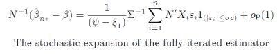
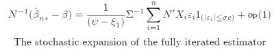
Moreover it follows from Johansen and Nielsen [
19] that, for the case of known
and symmetric density, the Huber skip has the stochastic expansion
and hence the same asymptotic distribution as
Finally the asymptotic distribution of
and therefore
is discussed in
Section 4.
2.2. Assumptions for the Asymptotic Analysis
The assumptions are fairly general, in particular we do not assume that is symmetric.
Assumption A Consider model (2.1). Assume
The density has continuous derivative and satisfies- (a)
- (b)
it has mean zero, variance one, and finite fourth moment,
- (c)
are chosen so and
For a suitable normalization matrix the regressors satisfy, jointly,- (a)
- (b)
- (c)
The initial estimator error satisfies 3. The Fixed Point Result
The fixed point result is primarily a tightness result. Thus, for the moment, only tightness of the kernel
is needed, and it is not necessary to establish the limit distribution, which is discussed in
Section 4. The first result is a tightness result for the kernel, see (2.13).
Theorem 3.1 Suppose Assumption A holds. Then see (2.10) and (2.13), is tight, that is, The proof follows from Chebyshev’s inequality and the details are given in the
appendix.
The next result discusses one step of the iteration (2.14), and it is shown that the remainder term in (2.14) vanishes in probability uniformly in
Theorem 3.2 Let m be fixed. Suppose Assumption A holds for the initial estimator see (2.8). Then, for all , it holds thatwhere the remainder term satisfies The proof involves a chaining argument that was given in Johansen and Nielsen [
6], although there the result was written up in a slightly different way as discussed in the
appendix.
The iterated estimators start with an initial estimator with tight estimation error, see Assumption A(). This is iterated through the one-step (2.14) and defines the sequence of estimation errors . We next show that this sequence is tight uniformly in
Theorem 3.3 Suppose Assumption A holds and that a.s. so that Γ
is a contraction. Then the sequence of estimation errors is tight uniformly in mThat is, for all there exist and so that for all it holds that The proof is given in the
appendix, but the idea of the proof is to write the solution of the recursive relation (2.14) as
Then, if the initial estimator takes values in a large compact set with large probability, it follows from (3.1), by finite induction, that also takes values in the same compact set for all , and therefore is tight uniformly in .
Finally we give the fixed point result. Theorem 3.4 shows that the estimator has the same limit distribution as the solution of equation (2.15), which is a fixed point of the linear function
Theorem 3.4 Suppose Assumption A holds and that a.s. so that Γ
is a contraction. ThenThat is, for all ϵ and an and exist so that for all and it holds Using
we find from (3.1) that
From (3.2) it can be seen that
is the sum of two terms vanishing in probability, where the first decreases exponentially. The details are given in the
Appendix.
In the special case where σ is known, then reduces to and and becomes a fixed point of the mapping defined in (2.4). The estimator appears as the leading term for other robust estimators, such as the Least Trimmed Squares estimator discussed later on.
A necessary condition for the result is that the autoregressive coefficient matrix Γ is contracting. Therefore Γ is analyzed next.
Theorem 3.5 The autoregressive coefficient matrix Γ
in (2.12) has eigenvalues equal to and two eigenvalues solvingwhere the coefficients and are given in (2.11).
Further results can be given about the eigenvalues of Γ for symmetric densities, where and . Note that the quantities all depend on see (2.2), (2.3), and (2.11). If is symmetric, we show below, that and a condition, is given for in which case the eigenvalues of Γ are less than one, and Γ isa contraction. Finally shows that Γ is a contraction if is log-concave.
Theorem 3.6 Suppose is symmetric with third moment, for and . Then
for while and
for and and
if for then for
The condition
is satisfied for the Gaussian density that is log-concave and by
t-densities that are not log-concave but satisfy
In the robust statistics literature, Rousseeuw uses the condition
when discussing change-of-variance curves for
M-estimators and assumes log-concave densities [
18].
A consequence of Theorem 3.6 is that if is symmetric, the roots of the coefficient matrix Γ are bounded away from unity for for all The uniform distribution on provides an example where Γ is not contracting since in this situation over the entire support. However, the weak unimodality condition in Theorem 3.6 is not necessary, as long as the mode at the origin is large in comparison with other modes.
4. Distribution of the Kernel
It follows from Theorem 3.4 that has the same limit as and we therefore find the limit distribution of the kernel in a few situations.
4.1. Stationary Case
Suppose the regressors are a stationary time series. Then the limits Σ and
μ in Assumption A
are deterministic and
. The central limit theorem then shows that
where
As a consequence, the fully iterated estimator has limit distribution
In the special case where the errors are symmetric, we find
noting that
and
are satisfied for symmetric, unimodal distributions by Theorem 3.6
The limiting distribution of is also seen elsewhere in the robust statistics literature.
First, Víšek [
15] (Theorem 1, p. 215) analysed the least trimmed squares estimator of Rousseeuw [
13]. The estimator is given by
where
are the ordered squared residuals
. The estimator has the property that it does not depend on the scale of the problem. Víšek argued that in the symmetric case, the least trimmed squares estimator satisfies
that is, the main term is the same as for
and it follows from Theorem 3.4 that because
and
have the same expansions we have
for
Thus
can be seen as an approximation to the
estimator when there are no outliers.
Second, Jurečková, Sen, and Picek [
4] (Theorem 5.5, p. 176) considered a pure location problem with regressor
and known
, and found an asymptotic expansion like (4.4) for the Huber-skip, and Johansen and Nielsen [
19] showed the similar result for the general regression model. A consequence of this is that the iterated 1-step Huber-skip has the same limit distribution as the Huber-skip, and because
and
have the same expansion, it follows from Theorem 3.4 that
so the iterated estimator is in this sense an approximation to the Huber-skip.
4.2. Deterministic Trends
As a simple example with i.i.d. errors, consider the regression
where
satisfies Assumption A
Define the normalisation
Then Assumption A
is met with
and
and
The kernel has a limit distribution given by (4.1), where the matrix Φ in (4.2) is computed in terms of the Σ and
μ derived in (4.6).
If the errors are autoregressive
, the derivation is in principle similar, but involves a notationally tedious detrending argument. The argument is similar to that of Johansen and Nielsen [
6] (Section 1.5.1), and (4.5) holds.
4.3. Unit Roots
Consider as an example the autoregression
If
then
and we have to choose
By the functional Central Limit Theorem
where the limit is a Brownian motion with zero mean and variance
Thus the limit variables Σ and
μ in Assumption A
are
while the kernel has limit distribution
and (4.5) holds. Thus, when the density of
is symmetric,
has limit distribution
When
then
and
so
and
become identical and the limit distribution becomes the usual Dickey–Fuller distribution. See also Johansen and Nielsen [
6] (Section 1.5.4) for a related and more detailed derivation.
5. Discussion of Possible Extensions
The iteration result in Theorem 3.4 has a variety of extensions. An issue of interest in the literature is whether a slow initial convergence rate can be improved upon through iteration. This would open up for using robust estimators converging for instance at a
rate as initial estimator. Such a result would complement the result of He and Portnoy, who find that the convergence rate cannot be improved in a single step by this procedure that applies least squares to the retained observations [
20].
The key is to show that the remainder term of the one-step estimator in Theorem 3.2 remains small in an appropriately larger neighbourhood. The proof of Theorem 3.4 then applies the same way leading to the same fixed point result. The necessary techniques are developed by Johansen and Nielsen [
21].
A related algorithm is the
Forward Search of Atkinson, Riani, and Cerioli [
7,
22]. This involves finding an initial set of “good” observations using for instance the least trimmed squares estimator of Rousseeuw [
13] and then increase the number of “good” observations using a recursive test procedure. The algorithm involves iteration of one-step Huber-skip estimators, see Johansen and Nielsen [
23]. Again the key to its analysis is to improve Theorem 3.2, in this instance to hold uniformly in the cut-off fraction
see Johansen and Nielsen for details [
21].
Another algorithm of interest would be to analyse algorithms such as
Autometrics of Hendry and Krolzig [
24] and Doornik [
25], which involves selection over observations as well as regressors.
In practice it is not a trivial matter to compute the least trimmed squares estimator of Rousseeuw [
13]. A number of algorithms have been suggested in the literature, see for instance Hawkins and Olive [
26]. Algorithms based on a “concentration” approach start with an initial trial fit that is iterated towards a final fit. It is possible that the abovementioned results will extend to shed some further light on the properties of such resampling algorithms.

